Test of the isotopic and velocity selectivity of a lithium atom interferometer by magnetic dephasing

Abstract

A magnetic field gradient applied to an atom interferometer induces a $M$-dependent phase shift which results in a series of decays and revivals of the fringe visibility. Using our lithium atom interferometer based on Bragg laser diffraction, we have measured the fringe visibility as a function of the applied gradient. We have thus tested the isotopic selectivity of the interferometer, the velocity selective character of Bragg diffraction for different diffraction orders as well as the effect of optical pumping of the incoming atoms. All these observations are qualitatively understood but a quantitative analysis requires a complete model of the interferometer.

If an inhomogeneous magnetic field is applied on a matter wave interferometer, the phase of the interference pattern is modified, provided that the matter wave has a non-zero magnetic moment. This type of situation was first considered [1, 2] as a test of the sign reversal of a spin $1/2$ wave function by a $2\pi$ rotation. This effect was predicted since the foundation of quantum mechanics but considered for a long time as not observable. The first successful experimental test was made by H. Rauch and co-workers [3] in 1975 with their perfect crystal neutron interferometer and this work has been followed by several other experiments reviewed in the book of Rauch and Werner [4].

Similar experiments can be done by applying a magnetic field gradient on an atom interferometer: the fringe patterns corresponding to the various Zeeman sub-levels experience different phase-shifts and, when the gradient increases, the fringe visibility exhibits a series of minima and recurrences, as first observed by D. Pritchard and co-workers [5, 6] and by Siu Au Lee and co-workers [7]. In this letter, we use our lithium atom interferometer to show that the dependence of the fringe visibility with the applied gradient gives a direct test of the selective character of our interferometer with respect to the atom velocity, to its isotopic nature and to its internal state distribution. The velocity selective character of our atom interferometer [8, 9] comes from the use of Bragg diffraction on laser standing waves. The choice of the laser wavelength gives access to the isotopic selectivity of the interferometer. Finally, by optical pumping ⁷Li in its $F=1$ ground state, we observe the effect of the internal state distribution on the visibility variations.

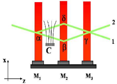
Figure 1: Schematic drawing of our Mach-Zehnder atom interferometer: a collimated atomic beam is diffracted by three laser standing waves, produced by reflecting three laser beams on three mirrors $M_{i}$. The output beams labelled $1$ and $2$ are complementary, one of them (usually beam $1$) being detected. A coil $C$ close to the atomic beams creates a magnetic field gradient in the $\mathbf{x}$-direction.

1 Calculation of the magnetic dephasing effect

A Mach-Zehnder atom interferometer, as represented in figure 1, is operated with a paramagnetic atom. If the magnetic field direction varies slowly enough, no spin flip occurs during the atom propagation and the projection $M_{F}$ of the total angular momentum $\mathbf{F}$ remains a good quantum number, the quantization axis being parallel to the local magnetic field. In the presence of a transverse gradient of the magnetic field, the Zeeman energy $\Delta E\left(F,M_{F}\right)$ of the $F,M_{F}$ sub-level is not the same on the two atomic paths and, in the perturbative limit (Zeeman energy considerably smaller than the atom kinetic energy $\hbar^{2}k^{2}/2m$), this energy difference induces a phase shift equal to:

$$\Delta\phi\left(F,M_{F}\right)=-\frac{1}{\hbar v}\oint\Delta E\left(F,M_{F},s\right)ds$$ (1)

where the path integral follows the $\alpha\beta\gamma\delta\alpha$ circuit (see figure 1) and $v$ is the atom velocity. The interferometer signal is the incoherent sum of the signals due to the various $F,M_{F}$ sub-levels:

$$I = \sum_{F,M_{F}}\int dvI\left(F,M_{F},v\right)$$

$$I\left(F,M_{F},v\right) = I_{0}P\left(v\right)P\left(F,M_{F}\right)\times[1+{\mathcal{V}}_{0}\cos\left(\psi+\Delta\phi\left(F,M_{F}\right)\right]$$ (2)

$I\left(F,M_{F},v\right)$ is the contribution of the $F,M_{F}$ atoms with the velocity $v$. $P\left(F,M_{F}\right)$ and $P(v)$ represent the internal state and velocity distribution of the output flux. The fringe visibility ${\mathcal{V}}_{0}$ is assumed to be independent of the sub-level. Finally, the origin of phase $\psi$ is explained below. We simplify the present discussion by assuming that the Zeeman energy $\Delta E\left(F,M_{F}\right)$ is a linear function of the field $B$:

$$\Delta E\left(F,M_{F}\right)=-g_{F}\mu_{B}M_{F}B$$ (3)

but our calculations take into account the non-linear Zeeman terms due to hyperfine uncoupling which are non-negligible, especially for ⁶Li. $\mu_{B}$ is the Bohr magneton and $g_{F}$ is the Landé factor equal to $g_{F}=+2/3$ (resp. $-2/3$) for the $F=3/2$ (resp. $F=1/2$) level of ⁶Li and $g_{F}=+1/2$ (resp. $-1/2$) for the $F=2$ (resp. $F=1$) level of ⁷Li, where the nuclear magnetic moments have been neglected. The phase shift $\Delta\phi\left(F,M_{F}\right)$ is given by:

$$\Delta\phi\left(F,M_{F}\right)=\frac{g_{F}\mu_{B}M_{F}}{\hbar v}\int_{z_{\alpha}}^{z_{\gamma}}\frac{\partial\left|B(z)\right|}{\partial x}\Delta x(z)dz$$ (4)

where $\Delta x(z)$ is the distance between the two atomic beams in the interferometer and the integral is taken along a path at mid-distance between the two paths $\alpha\beta\gamma$ and $\alpha\delta\gamma$ followed by each atom in the interferometer.

As the coil used to create the magnetic field is small, the magnetic gradient is important in a region where the field due to the coil is substantially larger than the ambient field, which can be neglected in the calculation. We have verified that this approximation is good. The phase shift is then proportional to the coil current $\mathcal{I}$ and to $v^{-2}$. One $v$ factor, apparent in equation (1), comes from the time spent in the perturbation. The other $v$ factor comes from the distance $\Delta x(z)$, proportional to the diffraction angle $\theta_{diff}=2ph/(mva)$, where $p$ is the diffraction order and $a$ the grating period. We thus get:

$$\Delta\phi\left(F,M_{F}\right)=C\frac{pg_{F}M_{F}\mathcal{I}}{mv^{2}}$$ (5)

where $C$ gathers several constant factors. It is interesting to note that the equations (1-5) are valid for bosons as well as for fermions. In the introduction, we have recalled the discussion of the $4\pi$ symmetry of fermions [1, 2] and the fact that our equations take the same form for bosons and fermions may seem in contradiction with well known results. The explanation of this apparent contradiction lies in the fact that the phase shift $\Delta\phi\left(F,M_{F}\right)$ is the product of a rotation angle by the $M_{F}$ value. For fermions, $M_{F}$ is an half-integer and the rotation angle must be equal to a multiple of $4\pi$ for a revival while the rotation angle must only be a multiple of $2\pi$ for bosons.

We assume that the velocity distribution is given by:

$$P(v)=\frac{S_{\|}}{u\sqrt{\pi}}\exp\left[-\left((v-u)S_{\|}/u\right)^{2}\right]$$ (6)

where $u$ is the most probable velocity and $S_{\|}$ the parallel speed ratio. This formula is used for supersonic beams [12] but we have omitted a $v^{3}$ pre-factor, which has minor effects when $S_{\|}^{2}$ is large , which is the case here. The parallel speed ratio $S_{\|}$ can be varied by changing the pressure in the supersonic beam source or the nozzle diameter and the velocity distribution can be directly measured thanks to Doppler effect by laser induced fluorescence of the lithium beam [10, 11].

Moreover, in the present calculations, $P(v)$ describes in fact the product of the initial beam velocity distribution $P_{i}(v)$ by the transmission $T(v)$ of the atom interferometer. Our calculations show that the transmission $T(v)$ is roughly a Gaussian function of the velocity around a velocity corresponding to the Bragg condition.

2 Some experimental details

Our atom interferometer [8, 9] is a three grating Mach-Zehnder interferometer. We use a supersonic beam of argon seeded with natural lithium ($92.4$% of ⁷Li and $7.6$% of ⁶Li). In the absence of optical pumping, the lithium atoms are equally distributed over the $F,M_{F}$ hyperfine sub-levels of their $2S_{1/2}$ ground state. The lithium mean velocity $u$ is $u\approx 1065$ m/s. The gratings being laser standing waves, their period $a$ is equal to half the laser wavelength $\lambda_{L}\approx 671$ nm, chosen very close to the first resonance line of lithium. We do not reiterate here the laser beam parameters which are given in the full description of our interferometer [9]. The phase of the interference fringes depends on the $x$-position of the gratings depending themselves on the position $x_{i}$ of the mirrors $M_{i}$ forming the three laser standing waves: this is the origin of the phase term $\psi$ in equation (1), $\psi=2pk_{L}(x_{1}+x_{3}-2x_{2})$, where $k_{L}=2\pi/\lambda_{L}$ is the laser wavevector and $p$ is the diffraction order. Figure 2 shows experimental interference fringes, observed by scanning the position $x_{3}$ of mirror $M_{3}$ (this is the usual way of observing fringes in atom interferometers as this phase is independent of atom velocity).

Figure 2: Interference fringes recorded corresponding to different currents, $\mathcal{I}=0$ A (squares) and $\mathcal{I}=1.4$ A (triangles), and their fits (full curves). The interferometer was tuned for ⁷Li with first order diffraction. The phase shift between the two experiments is very close to $\pi$, corresponding to a visibility inversion. Each data point corresponds to a $0.1$ s counting time. A few isolated data points, due to bursts of the hot-wire detector, are not included in the fits. The dotted line gives the mean value of the detector background, recorded by flagging the beam.

The magnetic field gradient is produced by a $3$ cm diameter coil, with its axis at $4$ cm before the second laser standing wave. On the coil axis, the distance $\Delta x$ between the two atomic beams is about $94$ $\mu$m. The ambient field is roughly equal to the Earth magnetic field with a $\sim 4\times 10^{-5}$ Tesla vertical component and a smaller horizontal component. From the coil dimensions, we can calculate the magnetic field and its gradient everywhere, but the distance of the coil to the atomic beams, about $0.7$ cm, is not accurately known and we will consider the constant $C$ appearing in equation 5 as an adjustable parameter. With our maximum current $\mathcal{I}=9$ A, the maximum field seen by the atoms is $B\approx 1.3\times 10^{-3}$ T, sufficient to introduce some hyperfine uncoupling, especially for ⁶Li isotope. As already stated, this effect is taken into account in our calculations

During an experiment, we first optimize the interferometer fringes with a vanishing coil current $\mathcal{I}=0$, then we record a series of interference signals as in figure 2, with increasing values of $\mathcal{I}$. Slow drifts of the fringe phase and visibility are corrected by frequent recordings with $\mathcal{I}=0$. From each recording, we can extract the phase and the visibility of the interference pattern, from which we deduce the effects of the applied field gradient, namely the relative visibility ${\mathcal{V}}_{r}(\mathcal{I})={\mathcal{V}}(\mathcal{I})/{\mathcal{V}}(\mathcal{I}=0)$ and also the phase shift $\Delta\phi(\mathcal{I})$ which will be discussed in another paper.

3 Test of the isotopic selectivity

Here, we compare two experiments involving the two isotopes of lithium and using first order diffraction $p=1$. We tune the interferometer by choosing the laser wavelength, for ⁷Li on the blue side (at $3$ GHz) of ²S_1/2 - ²P_3/2 transition of ⁷Li and, for ⁶Li, on the red side (at $2$ GHz) of ²S_1/2 - ²P_3/2 transition of ⁶Li. The nearest transition of the other isotope is detuned from the laser by $14$ GHz in the first case and $12$ GHz in the second case. The relative visibility is plotted as a function of the current $\mathcal{I}$ in figure 3 for both isotopes. The $\mathcal{I}=0$ visibility is quite different for the two isotopes: ${\mathcal{V}}(\mathcal{I}=0)\approx 75$% for ⁷Li and ${\mathcal{V}}(\mathcal{I}=0)\approx 48$% for ⁶Li. The best visibility achieved with lithium ⁷Li is ${\mathcal{V}}\approx 84.5$% [9], mostly limited by phase noise due to vibrations [14], and the present value is less good, because of small misalignments. The smaller visibility with ⁶Li is due to stray ⁷Li atoms arriving on the detector after diffraction by the second and third laser standing waves. The variations of the visibility ${\mathcal{V}}_{r}$ have a very different dependence with the current $\mathcal{I}$ for the two isotopes, an obvious consequence of the differences in the number of sub-levels with a given $M_{F}$ value and in the Landé factors. We have fitted these results using equations (1) and (1) with only two adjustable parameters, namely the distance of the coil center to the atomic beams and the parallel speed ratio $S_{\|}$ appearing in equation (5). The agreement with the experimental data is good, the discrepancy appearing mostly in the case of ⁶Li, when the visibility is very small.

Figure 3: Relative visibility ${\mathcal{V}}_{r}$ as a function of the applied current for ⁷Li (left panel) and ⁶Li (right panel). Experimental data points are represented by dots and the fits by full curves.

The fits of figure 3 assume that the signal comes only from the isotope selected by the chosen laser frequency. As ⁷Li is considerably more abundant than ⁶Li ( $92.4$% vs $7.6$%), this is, not surprisingly, an excellent assumption for the dominant isotope ⁷Li, but this assumption works well also with the less abundant isotope, ⁶Li. Assuming that the fringe patterns of the two isotopes are always in phase, we can estimate the contribution of ⁷Li isotope to the ⁶Li experiment: from the fit, we deduce a contribution less than $10$% of the fringe signal. We have developed a full model of the interferometer to explain this effect because a simple model, with Gaussian laser beams described as top-hat beams, cannot explain such a large isotopic selectivity.

4 Test of velocity selectivity

For this test, we have optically pumped ⁷Li in its $F=1$ state, using a diode laser tuned on the ²S_1/2, $F=2$ - ²P_3/2 transition. Optical pumping must be performed before collimation of the atomic beam, because the photon momentum transfers due to absorptions and emissions of photons would spoil the necessary sub-recoil collimation. In the analysis, we assume that the three $M_{F}$ sub-levels of the $F=1$ states are equally populated. We have recorded the fringe visibility using successively the diffraction orders $p=1$ and $p=2$, with different adjustments of the laser standing waves (beam diameters power density, frequency detuning and mirror directions, see ref. [9]). The measured relative visibility ${\mathcal{V}}_{r}(\mathcal{I})$ is plotted as a function of the coil current $\mathcal{I}$ in figure 4: the variations are very different from those observed on ⁷Li without optical pumping (see figure 3), because now only two $|M_{F}|=1$ sub-levels and one $M_{F}=0$ sub-level are populated. When the magnetic field gradient is large, $M_{F}\neq 0$ sub-levels experience a large phase shift so that their contribution to the fringe signal is washed out by the velocity average and the remaining fringe visibility is solely due to the $M_{F}=0$ sub-level. We thus predict that ${\mathcal{V}}_{r}$ tends toward $1/3$ in this case because there is one $M_{F}=0$ sub-level over the three sub-levels of $F=1$.

Figure 4: Relative visibility ${\mathcal{V}}_{r}$ (dots) of the interference fringes for ⁷Li, pumped in its $F=1$ ground state, as a function of the coil current. Experimental data points are represented by dots and the fits by full curves. Left panel: first order diffraction $p=1$, with a rapid decay of the revival intensity; right panel: second order diffraction $p=2$, with more apparent revivals. The asymptotic ${\mathcal{V}}_{r}=1/3$ value is represented by a dashed line.

As discussed above, the parameter which governs the decay of the revivals is the parallel speed ratio and a fit of these data gives $S_{\|}=9.0$ when using the first order diffraction, $p=1$, and $S_{\|}=14.5$ when using second order diffraction, $p=2$. The beam source conditions [9] were the same in both cases and, from our study of the lithium beam [10, 11], we know the initial value of the parallel speed ratio, $S_{\|i}\approx 8.5$ . The velocity selective character of Bragg diffraction appears to be strong for second order diffraction.

5 Conclusions

In this letter, we have studied the effects of a magnetic field gradient on the signals of a lithium atom interferometer and we have analyzed the resulting variations of the fringe visibility. Following Siu Au Lee and co-workers [7], we use a coil to produce the magnetic field gradient rather than a septum carrying an electric current and inserted between the two atomic beams as done by D. Pritchard and co-workers [5, 6]: the coil does not require the fine alignment of the septum and the two arrangements appear to give very similar effects.

The idea that such an experiment can measure the relative width of the velocity distribution was pointed out by J. Schmiedmayer et al. [6]. We have applied this idea with our laser diffraction atom interferometer and we have observed a modification of the velocity distribution due to Bragg diffraction by comparing first and second diffraction orders. We have shown that the visibility variations give access to other quantities, such as the interferometer isotopic selectivity, which is excellent in our experiment with a correct choice of laser detuning. Finally, optical pumping modifies strongly the visibility variations, in good agreement with simple arguments. The ability to test the velocity distribution or the isotopic selectivity will be very useful for the following reasons:

- as discussed after equation (6), the velocity distribution of the atoms contributing to the interference signals differs from the velocity distribution of the incident atomic beam and this difference is very important for accurate phase shift measurements because most phase shifts are dispersive (proportional to $v^{n}$ with $n=-1$ as in a measurement of an electric polarizability [13] or $n=-2$ as in the present experiments).

- a test of the isotopic selectivity distribution could also be useful to measure the isotopic dependence of some quantity, for instance the electric polarizability. This possibility has presently little interest because this dependence is considerably smaller than the present accuracy [13] but it might not be always so.

- [1] Y. Aharonov and L. Susskind, Phys. Rev. 158, 1237 (1967)
- [2] H. J. Bernstein, Phys. Rev. Lett. 18, 1102 (1967)
- [3] H. Rauch, A. Zeilinger, G. Badurek, A. Wilfing, W. Bauspiess and U. Bonse, Phys. Lett. A 54, 425 (1975)
- [4] H. Rauch and S. Werner, Neutron Interferometry, Clarendon Press (Oxford, 2000) p. 165.
- [5] J. Schmiedmayer, C. R. Ekstrom, M. S. Chapman, T. D. Hammond, and D. E. Pritchard, J. Phys. II, France 4, 2029 (1994)
- [6] J. Schmiedmayer, M. S. Chapman, C. R. Ekstrom, T. D. Hammond, D. A. Kokorowski, A. Lenef, R. A. Rubinstein, E. T. Smith and D. E. Pritchard, in Atom interferometry edited by P. R. Berman (Academic Press 1997), p. 1
- [7] D. M. Giltner, R. W. McGowan and Siu Au Lee, Phys. Rev. A 52, 3966 (1995) and D. M. Giltner, Ph. D. thesis, University of Colorado at Fort Collins (1996), unpublished
- [8] R. Delhuille, C. Champenois, M. Büchner, L. Jozefowski, C. Rizzo, G. Trénec and J. Vigué, Appl. Phys. B 74, 489 (2002)
- [9] A. Miffre, M. Jacquey, M. Büchner, G. Trénec and J. Vigué, Eur. Phys. J. D 33, 99 (2005)
- [10] A. Miffre, M. Jacquey, M. Büchner, G. Trénec and J. Vigué, Phys. Rev. A 70, 030701(R) (2004),
- [11] A. Miffre, M. Jacquey, M. Büchner, G. Trénec and J. Vigué, J. Chem. Phys. 122, 094308 (2005)
- [12] H. Haberland, U. Buck and M. Tolle, Rev. Sci. Instrum. 56, 1712 (1985)
- [13] A. Miffre, M. Jacquey, M. Büchner, G. Trénec and J. Vigué, Phys. Rev. A 73, 011603(R) (2006) and Eur. Phys. J. D 38, 353 (2006)
- [14] M. Jacquey, A. Miffre, M. Büchner, G. Trénec and J. Vigué, Europhys. Lett. 75, 688 (2006)