Abstract

We consider a pair of antiparallel spins polarized in a random direction to encode quantum information. We wish to extract as much information as possible on the polarization direction attainable by an unentangled measurement, i.e., by a measurement, whose outcomes are associated with product states. We develop analytically the upper bound $0.7935$ bits to the Shannon mutual information obtainable by an unentangled measurement, which is definitely less than the value $0.8664$ bits attained by an entangled measurement. This proves our main result, that not every ensemble of product states can be optimally distinguished by an unentangled measurement, if the measure of distinguishability is defined in the sense of Shannon. We also present results from numerical calculations and discuss briefly the case of parallel spins.

PACS numbers: 03.67.Mn, 03.65.Ta

1 Introduction

One of the central problems in quantum information theory is the state discrimination problem. Suppose that one is given a single quantum system, which is known to be in one of several possible states with a certain a priori probability. Then one wishes to carry out such a measurement on the system that would yield as much information about the identity of the system’s state as possible, where the gained information is defined in terms of the Shannon mutual information.

Although there exist other figures of merit, which quantify distinguishability, such as the statistical overlap (i.e., the fidelity), or the Kullback-Leibler relative information [1, 2], in this work we will focus on the mutual information, which quantifies the quality of measurement through the average gain of information about the unknown states [3, 4].

A particular instance of the discrimination problem is when each possible state of the system is restricted to be in a product state. With regard to this, some time ago Peres and Wootters [5] addressed the intriguing problem of whether in order to gain as much information as possible from an ensemble of product states it is sufficient to do local measurements or sometimes necessary to carry out a global measurement on the system as a whole. Technically, in the first case one is permitted to do any sequence of local operations carried out on each subsystem individually and classical communication between the subsystems (LOCC), while in the second case arbitrary quantum operations are allowed on both spins.

Hitting upon a special ensemble of states, the double-trine states, they showed evidence that a global measurement was distinctly better than any LOCC measurement. Recently, Decker [6] confirmed this result and other studies [7, 8, 9] also proved conclusively the superiority of global measurements over LOCC measurements, for which property the phrase “quantum nonlocality without entanglement” was coined [7].

While in the above case, a distinction was made between the power of global and local measurements, one may further divide global measurements into the following two distinct classes: Unentangled measurements, whose outcomes are associated with product states, and entangled measurements, for which at least one outcome is associated with an entangled state. An interesting question was posed recently by Wootters [10] of whether every ensemble of product states could be distinguished just as well by an unentangled measurement as by an entangled measurement. Although it turned out [10], that an unentangled measurement on the double-trine ensemble was as good as an entangled measurement, the question remained open about the existence of other kinds of product states where the best unentangled measurement could be beaten by an entangled one.

In the present article we wish to address this general question by focusing on the following special state discrimination problem: Given a source, which emits a pair of antiparallel spin-$1/2$ particles (spins for short) polarized along a random space direction, the observer’s task is to perform an unentangled measurement on the two spins which provides the maximum gain of information about the polarization direction. In the present study we manage to bound from above the maximum gain of information attainable by an unentangled measurement on two antiparallel spins, and this upper bound will appear to be smaller than the information which can be extracted by a particular entangled measurement. With this result we intend to give an answer for the question raised above, that on product states entangled measurements are in general more informative than unentangled ones. Further, since the set of unentangled measurements is strictly larger than the set of LOCC measurements [7], the pair of antiparallel spins can be considered as another example beside the double-trine ensemble, where global measurements are distinctly more powerful than LOCC measurements.

Note that the state discrimination of antiparallel spins discussed above can be interpreted as a quantum communication problem, i.e., the problem of communicating an unknown spatial direction between two distant parties by the transmission of quantum particles. This problem has been extensively studied in the literature [11, 12, 13, 14, 15, 16, 17], but using the fidelity as a figure of merit. Our findings corresponding to the mutual information thus can also be regarded as a complement to the results of the cited references.

The article is organized as follows: In Sec. 2 we introduce the notation and formulate the problem. In Sec. 3 the rotational invariance property of the mutual information is demonstrated and the problem of obtaining the best unentangled measurement is presented as a constrained optimization problem. In Sec. 4 the optimization is performed by the Lagrange multipliers method by applying Jensen’s inequality. Then the best unentangled measurement is given explicitly in terms of measurement projectors and we also discuss briefly the case of two parallel spins. The paper concludes in Sec. 5 with a discussion of the results.

2 Formalism

2.1 POVM measurement

As we mentioned in the Introduction our state discrimination problem can be presented as a quantum communication task: Suppose Alice wishes to communicate to Bob a spatial direction, i.e., a unit vector $\mathbf{n}$ chosen completely at random. In order to accomplish the task, Alice prepares two spins in the product state

$$|A(\mathbf{n})\rangle=|\mathbf{n}\rangle|-\mathbf{n}\rangle\;,$$ (1)

where the first spin is polarized along the random space direction $\mathbf{n}$ and the second spin is polarized in the opposite direction $-\mathbf{n}$. Then she sends the pair of antiparallel spins to Bob, and upon receiving it Bob performs an unentangled measurement on the spins so as to acquire as much knowledge about the spatial direction $\mathbf{n}$ as possible. The polarized spin state $|\mathbf{n}\rangle$ corresponding to Alice’s signal satisfies

$$\hat{\sigma}\cdot\mathbf{n}|\mathbf{n}\rangle=|\mathbf{n}\rangle\;,$$ (2)

where $\hat{\sigma}$ are the usual Pauli matrices.

On the other hand, the mathematical representation of Bob’s measurement apparatus is a positive operator valued measure (POVM) consisting of a set of operators $E_{r}$, which sum up to unity on the four-dimensional Hilbert space of the two spins,

$$\sum_{r=1}^{M}{E_{r}=\mathbb{I}}\;,$$ (3)

where $r=1,\ldots,M$ labels the outcome of the measuring process and we require $M\geq 4$ owing to the size of the Hilbert space. Note that the sum in Eq. (3) can be extended to the continuous case as well by a suitable adjustment of the notation. Taking into account that one can always assume the projectors $E_{r}$ to have rank one [18], we can write

$$E_{r}=c_{r}|\psi_{r}\rangle\langle\psi_{r}|\;,$$ (4)

where $c_{r}$ are positive weights and states $|\psi_{r}\rangle$ are normalized. Bob is allowed to carry out unentangled measurements, i.e., measurements for which each of the POVM operator elements $E_{r}$ is a tensor product. Thus each state $|\psi_{r}\rangle$ corresponding to measurement outcome $r$ can be written in the product form

$$|\psi_{r}\rangle=|\mathbf{n}_{1r}\rangle|\mathbf{n}_{2r}\rangle\;.$$ (5)

The pairs of unit vectors $\mathbf{n}_{1r}$ and $\mathbf{n}_{2r}$ are yet free parameters, which must be adjusted by Bob appropriately so as to achieve the highest possible amount of mutual information between the outcomes of his unentangled measurement and Alice’s states. In order to arrive at an explicit formula for this information gain let us introduce some notations.

2.2 Information gain

The conditional probability $p(r|\mathbf{n})$ that Alice’s preparation $|A(\mathbf{n})\rangle$ yields Bob’s result $r$ is given by Born’s rule

$$p(r|\mathbf{n})=c_{r}|\langle A(\mathbf{n})|\psi_{r}\rangle|^{2}\;,$$ (6)

which on substitution the signal state (1) and Bob’s product states (5) into this expression gives

$$p(r|\mathbf{n})=c_{r}|\langle\mathbf{n}|\mathbf{n}_{1r}\rangle|^{2}|\langle-\mathbf{n}|\mathbf{n}_{2r}\rangle|^{2}\;.$$ (7)

Let us designate an arbitrary point $(\theta,\phi)$ on the Bloch sphere by the unit vector $\mathbf{n}(\theta,\phi)$ specified by the coordinates $\mathbf{n}=(\cos\phi\sin\theta,\sin\phi\sin\theta,\cos\theta)$. Since Alice chooses $\mathbf{n}$ randomly, or say equivalently, Bob has no knowledge before his measurement about the space direction $\mathbf{n}$ which Alice indicates by her signal (1), it entails the uniform a priori distribution $p(\mathbf{n})=1$ on the Bloch sphere.

The a priori probability that Bob has measurement outcome $r$ is

$$p(r)=\int{dnp(r|\mathbf{n})p(\mathbf{n})}\;,$$ (8)

where the integration is performed over the whole Bloch sphere and $dn=\frac{1}{4\pi}\sin\theta d\theta d\phi$ is the uniform measure on the Bloch sphere. Then applying Bayes’ theorem the a posteriori probability for $\mathbf{n}$ is given by

$$p(\mathbf{n}|r)=\frac{p(r|\mathbf{n})}{p(r)}p(\mathbf{n}).$$ (9)

The Shannon mutual information is the average amount of information that one gains about the direction $\mathbf{n}$ upon observing the outcome of the measurement. Thus it can be written as the difference of the a priori entropy $H_{initial}$ of $p(\mathbf{n})$ and the average a posteriori entropy $\bar{H}_{final}$ of $p(\mathbf{n}|r)$ [3, 4].

The value of $H_{initial}$ is infinite for the continuous distribution $p(\mathbf{n})$, but as it can be shown [3, 24] the divergent term is cancelled by terms from $\bar{H}_{final}$ and the Shannon mutual information can be expressed in the closed form [19, 20, 21]

$$I_{av}=\sum_{r=1}^{M}{p(r)K\left(p(\mathbf{n}|r)/p(\mathbf{n})\right)}\;,$$ (10)

in terms of the Kullback-Leibler relative information between the distributions $p(\mathbf{n}|r)$ and $p(\mathbf{n})$,

$$K\left(p(\mathbf{n}|r)/p(\mathbf{n})\right)=\int{dnp(\mathbf{n}|r)\log_{2}\frac{p(\mathbf{n}|r)}{p(\mathbf{n})}}\;.$$ (11)

Our starting point is this information gain, Eq. (10), to quantify Bob’s measuring strategy, which is well-defined for continuous distributions [22]. Particularly, we intend to optimize Eq. (10) by restricting Bob to perform an unentangled measurement described by Eq. (5) and considering that the a priori distribution of Alice’s ensemble is $p(\mathbf{n})=1$. However, we also want the projectors $E_{r}$ to constitute a valid POVM. This imposes the following pair of constraints, which Bob’s unentangled measurement operators must fulfill in order to optimize his gained information (10),

$$\sum_{r=1}^{M}{c_{r}}=4\;,\hskip 19.91692pt\sum_{r=1}^{M}{p(r)}=1\;,$$ (12)

where the first constraint is obtained by evaluating the trace of the POVM condition (3) considering Eq. (4), and the second constraint is due to the fact that $p(r)$ is a probability distribution.

3 Optimization problem

3.1 Rotational invariance

As a next step, we aim to exploit rotational invariance properties of the a priori probability $p(r)$ defined by Eq. (8) and the mutual information $I_{av}$ given by Eq. (10) in order that we could bring the state (5) to a simpler form. Regarding the uniform distribution $p(\mathbf{n})=1$ and substituting formula (7) into the definition (8) one obtains

$$p(r)=c_{r}\int{dn|\langle\mathbf{n}|\mathbf{n}_{1r}\rangle|^{2}|\langle-\mathbf{n}|\mathbf{n}_{2r}\rangle|^{2}}\;.$$ (13)

This formula, owing to the rotational invariance of the integral, is unchanged under an arbitrary collective rotation $R_{r}$ of the unit vectors $\mathbf{n}_{1r}$ and $\mathbf{n}_{2r}$, i.e.,

$$p(r)=c_{r}\int{dn|\langle\mathbf{n}|R_{r}(\mathbf{n}_{1r})\rangle|^{2}|\langle-\mathbf{n}|R_{r}(\mathbf{n}_{2r})\rangle|^{2}}\;.$$ (14)

For the same symmetry reasons the information gain (10) (with $p(\mathbf{n})=1$) also remains invariant by replacing $\mathbf{n}_{ir}\rightarrow R_{r}(\mathbf{n}_{ir}),\hskip 7.11317pti=1,2$. In particular, let us choose the rotations $R_{r}$ in such a way that

$$R_{r}(\mathbf{n}_{1r}) =\mathbf{z}\;,$$

$$R_{r}(\mathbf{n}_{2r}) =\mathbf{n}_{r}(\theta_{r},\phi_{r}=0)$$ (15)

for r = 1, …, M. That is, by a suitable collective rotation of the pair of unit vectors $\mathbf{n}_{1r}$ and $\mathbf{n}_{2r}$, one rotates $\mathbf{n}_{1r}$ into the north pole, while $\mathbf{n}_{2r}$ to a point, represented by $\mathbf{n}_{r}$, so that it lies on the polar great circle arc of the Bloch sphere. Since $R_{r}$ represents an arbitrary rotation, the rotations (15) can always be performed, also guaranteeing

$$\mathbf{z}\cdot\mathbf{n}_{r}=\mathbf{n}_{1r}\cdot\mathbf{n}_{2r}=\cos\theta_{r}\;,$$ (16)

where $\theta_{r}$ is the angle between the pair of vectors $\mathbf{n}_{1r}$ and $\mathbf{n}_{2r}$. Therefore, in effect the mapping of states

$$|\psi_{r}\rangle=|\mathbf{n}_{1r}\rangle|\mathbf{n}_{2r}\rangle\rightarrow|\tilde{\psi}_{r}\rangle=|\mathbf{z}\rangle|\mathbf{n}_{r}\rangle$$ (17)

induced by the collective rotations $R_{r}$ will not change the amount of information gain (10). Here $|\mathbf{n}_{r}\rangle$ can be written explicitly in the basis $\{|\mathbf{z}\rangle,|-\mathbf{z}\rangle\}$

$$|\mathbf{n}_{r}\rangle=\cos\frac{\theta_{r}}{2}|\mathbf{z}\rangle+\sin\frac{\theta_{r}}{2}|-\mathbf{z}\rangle$$ (18)

using relation (16).

3.2 Constrained formula

Let us make use of the informational equivalence which we found in the preceding subsection between $|\psi_{r}\rangle$ and $|\tilde{\psi}_{r}\rangle$ and make the replacement (17) for obtaining a simplified form of the information gain (10). Then by means of Eq. (17) and considering $p(\mathbf{n})=1$ the conditional probability $p(r|\mathbf{n})$ in Eq. (7) is mapped to

$$p(c_{r},\theta_{r}|\mathbf{n}) =c_{r}|\langle\mathbf{n}|\mathbf{z}\rangle|^{2}|\langle-\mathbf{n}|\mathbf{n}_{r}\rangle|^{2}$$

$$=\frac{c_{r}}{2}\cos^{2}\frac{\theta}{2}(1-\cos\theta\cos\theta_{r}-\cos\phi\sin\theta\sin\theta_{r})$$ (19)

and in turn the probability $p(r)$ becomes

$$p(c_{r},\theta_{r})=\int{dnp(c_{r},\theta_{r}|\mathbf{n})}=c_{r}\frac{3-\cos\theta_{r}}{12}\;,$$ (20)

where in Eq. (19) the variables $(c_{r},\theta_{r},\theta)$ are written out explicitly and were also used in the evaluation of Eq. (20).

Given Eqs. (19-20) the problem of optimizing Bob’s information gain (10) subject to the corresponding constraints (12) can be presented in terms of the variables $(c_{r},\theta_{r}),\hskip 7.11317ptr=1,\ldots,M$. Namely, after a bit of algebra and using $p(\mathbf{n})=1$ the information gain (10) quantified by the mutual information takes the explicit form

$$I_{av}=\sum_{r=1}^{M}{c_{r}I(\theta_{r})}\;,$$ (21)

where

$$I(\vartheta)=\frac{3-\cos\vartheta}{12}\int{dn\frac{p(c_{r},\vartheta|\mathbf{n})}{p(c_{r},\vartheta)}\log_{2}{\frac{p(c_{r},\vartheta|\mathbf{n})}{p(c_{r},\vartheta)}}}\;.$$ (22)

Note that as a consequence of Eqs. (19) and (20) the fraction $p(c_{r},\vartheta|\mathbf{n})/p(c_{r},\vartheta)$ and hence $I(\vartheta)$ within Eq. (22) are independent of the index $r$.

Since the information gain (21) is subjected to constraints we have to impose some restrictions on the domain of the variables $(c_{r},\theta_{r})$. On the one hand, these variables need to be in the range

$$(c_{r}>0,\;0\leq\theta_{r}\leq\pi),\hskip 14.22636ptr=1,\ldots,M\;,$$ (23)

where the number $M$ is at least $4$. On the other, the constraints (12) further restrict the domain and these conditions can be brought to the explicit forms

$$\sum_{r=1}^{M}{c_{r}}=4\;,\hskip 19.91692pt\sum_{r=1}^{M}{c_{r}\cos\theta_{r}}=1\;,$$ (24)

by replacing Eq. (8) with Eq. (20). In the following, let us refer to the domain, which is within the range (23) and satisfies constraints (24) as the feasible region.

To summarize this section, the information gain in Eq. (21) with the constraints (23-24) constitute the constrained optimization problem: Bob’s task is to maximize the mutual information (defined by Eq. (21)) between his unentangled measurement outcomes and Alice’s signals by choosing appropriately the set of values ${(c_{r},\theta_{r})}$ from the feasible region (defined by Eqs. (23-24)). The next section is centered on the problem of how to build a reasonable upper bound to this maximal amount of information gain.

4 Solution

4.1 Upper bound

The direct evaluation of the integral in Eq. (22) is an intractable task owing to the logarithm appearing in the integrand (a detailed analysis of the difficulties arising in an analytical treatment of the mutual information can be found in the PhD thesis of Fuchs [2]). However, applying Jensen’s inequality [2] it enables us to develop an upper bound to the function $I(\vartheta)$ given by Eq. (22) and to its weighted sum, the information gain (21). Jensen’s inequality involving a probability density function can be stated as follows [23]: If $g$ is any real valued measurable function, $f$ is a probability density function, and $\varphi$ is concave over the range of $g$, then

$$\int{dnf(\mathbf{n})\varphi(g(\mathbf{n}))\leq\varphi\left(\int{dnf(\mathbf{n})g(\mathbf{n})}\right)}\;.$$ (25)

Let the concave function $\varphi$ be particularly the logarithm function $\log_{2}x$, and let functions $f$ and $g$ be equal to the fraction ${p(c_{r},\vartheta|\mathbf{n})}/{p(c_{r},\vartheta)}$. As a result a complete correspondence can be established between the integral within Eq. (22) and the left-hand side of Eq. (25), entailing the upper bound $J(\vartheta)$ to the function $I(\vartheta)$ as follows:

$$I(\vartheta)\leq\frac{3-\cos\vartheta}{12}\log_{2}\left(\int{dn\left(\frac{p(c_{r},\vartheta|\mathbf{n})}{p(c_{r},\vartheta)}\right)^{2}}\right)\equiv J(\vartheta)\;.$$ (26)

Note that in contrast to the function $I(\vartheta)$, which can be computed only numerically, its upper bound $J(\vartheta)$ can be given in analytic terms. The respective curves of the function $I(\vartheta)$ and the function $J(\vartheta)$ are plotted in Fig. 1 in the range $0\leq\vartheta\leq\pi$.

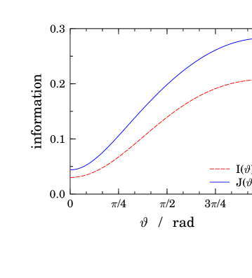
Figure 1: The function $I$ and its upper bound $J$ plotted against $\vartheta$ in the interval $0\leq\vartheta\leq\pi$.

After developing an upper bound to the information function $I(\vartheta)$ we wish to show that finding a global maximum of the function

$$J_{av}=\sum_{r=1}^{M}{c_{r}J(\vartheta_{r})}$$ (27)

in the feasible region (which region is defined in Subsection (3.2)) will serve as an upper bound to the global maximum of the information gain (21) in the same feasible region, i.e., to the amount of information which Bob can acquire by his best unentangled measurement.

To supply a proof, let us suppose the opposite, that is inside the feasible region the maximum value of $I_{av}$ is bigger than the maximum value of $J_{av}$. However, owing to the positive weights $c_{r}$ and the fact that $I(\vartheta)\leq J(\vartheta)$, by the definitions (21, 27) $I_{av}\leq J_{av}$ at any point of the feasible region. Thus, by means of this argument $I_{av}$ should also be upper bounded by $J_{av}$ at the very point of its maximum inside the feasible region, which contradicts our assumption, thereby completing the proof.

4.2 Lagrange multipliers

In this subsection, by the method of Lagrange multipliers we find via an analytical treatment the value of the global maximum of $J_{av}$ in the feasible region so as to provide an upper bound to the highest value of $I_{av}$ in the feasible region (as stated in the preceding subsection), achievable by an unentangled measurement. Thus we will obtain an upper bound to the amount of information which Bob can gain about Alice’s states by carrying out unentangled measurements.

To this end, let us introduce the Lagrange multipliers $\lambda_{1}$ and $\lambda_{2}$ which aim to account for the constraints (24). Note that inequality constraints (23) will instead be taken into account by restricting the domain of solutions. Then our task is to maximize the Lagrangian $L$,

$$L=\sum_{r=1}^{M}{c_{r}J(\theta_{r})}+\lambda_{1}\sum_{r=1}^{M}{c_{r}\cos\theta_{r}}+\lambda_{2}\left(\sum_{r=1}^{M}{c_{r}}-4\right)\;.$$ (28)

Variations of $L$ with respect to $\theta_{r}$ and $c_{r}$ yield the following two sets of equations,

$$\frac{\delta L}{\delta\theta_{r}}=0\;,\hskip 19.91692pt\frac{\delta L}{\delta c_{r}}=0\;,\hskip 19.91692ptr=1,\ldots,M\;,$$ (29)

which can be solved for $\lambda_{1}$ and $\lambda_{2}$, and we obtain

$$\lambda_{1} =\frac{1}{\sin\theta_{r}}\frac{dJ(\theta_{r})}{d\theta_{r}}\;,$$

$$\lambda_{2} =-J(\theta_{r})-\cot(\theta_{r})\frac{dJ(\theta_{r})}{d\theta_{r}}\;,\hskip 19.91692ptr=1,\ldots,M\;.$$ (30)

Let us define the function

$$h(\vartheta)=\frac{1}{\sin\vartheta}\frac{dJ(\vartheta)}{d\vartheta}\;.$$ (31)

Then the first equality within Eq. (30) becomes $\lambda_{1}=h(\theta_{r})$. Next our aim is to characterize $h(\vartheta)$ according to its monotonicity. Differentiating $h(\vartheta)$ with respect to $\vartheta$ we obtain the explicit formula

$$\frac{dh(\vartheta)}{d\vartheta}=\frac{-16}{3\ln 2}\frac{15-8\cos\vartheta+\cos 2\vartheta}{\left(27-20\cos\vartheta+\cos 2\vartheta\right)^{2}}\frac{\sin\vartheta}{3-\cos\vartheta}\;,$$ (32)

which is negative in the range $0<\vartheta<\pi$ (and zero at $\vartheta=0,\pi$) implying that $h(\vartheta)$ is a strictly decreasing function in the interval $0<\vartheta<\pi$. Further, according to Eq. (30), $h(\theta_{r})$ must be equal to a yet undetermined constant $\lambda_{1}$ for $r=1,\ldots,M$ at a stationary point (which can be either a point of local extremum or a saddle point) in the feasible region. Thus the monotonicity of $h(\vartheta)$ implies that at a stationary point in the feasible region all $\theta_{r}$ must be the same, that is one single solution exists for the variables $\theta_{r}$,

$$\theta_{r}=\theta_{opt}\hskip 19.91692ptr=1,\ldots,M\;.$$ (33)

In order to determine unambiguously $\theta_{opt}$ let us invoke constraints (24), which allow us to write at the above stationary point the following chain of equalities:

$$\sum_{r=1}^{M}{c_{r}\cos\theta_{r}}=\sum_{r=1}^{M}{4\cos\theta_{opt}}=4\cos\theta_{opt}=0\;.$$ (34)

Hence the last equality provides us with the explicit solution

$$\theta_{r}=\theta_{opt}=\frac{\pi}{2}\;,\hskip 19.91692ptr=1,\ldots,M$$ (35)

in the interval $[0,\pi]$, whereas the values of weights $c_{r}$ must satisfy the condition $\sum_{r=1}^{M}{c_{r}=4}$ (i.e., they are in the feasible region). Applying this solution (35) and the corresponding condition we may write at this stationary point for the value of $J_{av}$,

$$\max J_{av}=\sum_{r=1}^{M}{c_{r}J(\theta_{opt})}=4J(\pi/2)=0.7935\;\mathrm{bits}\;.$$ (36)

Now we wish to prove that the value of $\max J_{av}$ is a global maximum of the function $J_{av}$ inside the feasible region. Further, it is sufficient to show that it is a local maximum due to the single solution (35).

For this aim let us fix the values of $c_{r}$ in the feasible region, and evaluate the Hessian matrix of $J_{av}(\theta_{1},\dots,\theta_{M})$ at the point of the solution (35). After differentiations we obtain the Hessian as an $M\times M$ diagonal matrix whose $k$-th diagonal entry is given by $-56c_{k}/(1521\ln 2)$. Since the weights $c_{k}$ are positive, the Hessian matrix is negative definite implying that the solution (35) is a point of local maximum in an unrestricted domain of $\theta_{r}$ and consequently it is in the (smaller) feasible region as well.

This proves our proposition that $\max J_{av}=0.7935$ bits is a global maximum, which can be attained by the function $J_{av}$ subject to the constraints (23-24). Combining this result with the argument given in the previous subsection entails that the value $0.7935$ bits necessarily upper bounds the information gain (21) attainable by an unentangled measurement on Alice’s two antiparallel spins.

We found this upper bound by an analytical treatment, however by means of numerical calculations we may arrive as well at the maximum information gain $\max I_{av}$ attainable by an unentangled measurement if one replaces $I\rightarrow J$ in Eqs. (28-31). Owing to the logarithm in the integrand (22) this really needs numerical integration. Numerics shows that $h(\vartheta)$ will be a monotonic decreasing function in this case as well, providing the same stationary point (35) in the feasible region for the information gain $I_{av}$ as it was found before for its upper bound $J_{av}$. In the present case, however, we obtain

$$\max I_{av}=\sum_{r=1}^{M}{c_{r}I(\theta_{opt})}=4I(\pi/2)=0.557\;\mathrm{bits}\;.$$ (37)

By applying the same arguments for $I_{av}$ as for its upper bound $J_{av}$ and by evaluating the Hessian matrix (which can be done this time only numerically), we conclude that the solution (35) is a point of global maximum of $I_{av}$ in the feasible region (as for $J_{av}$), and therefore we can assert that the maximum mutual information between Bob’s unentangled measurement and Alice’s antiparallel spins is $\max I_{av}=0.557$ bits.

In the next subsection we discuss the concrete form of the POVMs which corresponds to the solution (35), implying that the values $\max I_{av}=0.557$ bits and $\max J_{av}=0.7935$ bits indeed correspond to a realizable measurement.

4.3 POVMs

Our aim is to obtain those POVM elements $E_{r}$ within Eq. (3) which produce Bob’s best unentangled measurement. For this, we substitute the solution (35) into Eq. (18) and as a result the mapped states $|\tilde{\psi_{r}}\rangle$ in Eq. (17) become

$$|\tilde{\psi_{r}}\rangle=|\mathbf{z}\rangle\left(\frac{|\mathbf{z}\rangle+|-\mathbf{z}\rangle}{\sqrt{2}}\right)\equiv|B\rangle\;,$$ (38)

i.e., each of them turns out to be the same ($r$ independent) reference state $|B\rangle$. Now, inverting the map (17) and defining the unit vectors $\mathbf{m}_{r}$ through the arbitrary spatial rotations $\mathbf{m}_{r}=R_{r}(\mathbf{z})$ yield

$$|\psi_{r}\rangle=|\mathbf{m}_{r}\rangle\left(\frac{|\mathbf{m}_{r}\rangle+|-\mathbf{m}_{r}\rangle}{\sqrt{2}}\right)\;.$$ (39)

Let us try with a minimal measurement, i.e., a measurement which has the minimum number $M=4$ of POVM elements. This corresponds to a von Neumann measurement satisfying the orthogonality requirement $E_{r}E_{s}=E_{r}\delta_{rs}$. Consequently, $\langle\psi_{r}|\psi_{s}\rangle=\delta_{rs}$ implying $c_{r}=1,\;r=1,2,3,4$ (in accord with conditions in Eqs. (23-24) for $c_{r}$). Now we are left with finding the angles $(\theta_{r}^{m},\varphi_{r}^{m})$ defining directions $\mathbf{m}_{r},\;r=1,2,3,4$, so as to completely define the POVM elements. If we choose the angles $(\theta_{r}^{m},\varphi_{r}^{m})$ to be

$$(0,0)\hskip 14.22636pt(0,\pi)\hskip 14.22636pt(\pi,0)\hskip 14.22636pt(\pi,\pi)\;,$$ (40)

it can be verified that the corresponding states $|\psi_{r}\rangle$ in Eq. (39) indeed constitue a legitimate POVM, $\sum_{r=1}^{4}{|\psi_{r}\rangle\langle\psi_{r}|}=\mathbb{I}$. The measuring strategy described by this unentangled POVM is in fact an LOCC measurement: Bob makes a von Neumann measurement of Alice’s first spin along an arbitrary direction (say $\mathbf{z}$) and of Alice’s second spin along an orthogonal direction.

On the other hand, Bagan et al. [24] found that for a pair of antiparallel spins a measurement strategy which yields the maximal fidelity, at the same time attains the value $0.8664$ bits of the mutual information . The corresponding POVM measurement is a von Neumann type, described by the projectors $E_{r}=|\psi_{r}\rangle\langle\psi_{r}|$ as follows [14],

$$|\psi_{r}\rangle=\frac{\sqrt{3}}{2}\frac{|\mathbf{m}_{r}\rangle|-\mathbf{m}_{r}\rangle+|-\mathbf{m}_{r}\rangle|\mathbf{m}_{r}\rangle}{\sqrt{2}}+\frac{1}{2}|\psi^{-}\rangle\;,\hskip 17.07164ptr=1,2,3,4\;,$$ (41)

where the four unit vectors $\mathbf{m}_{r}$ are pointing to the vertices of a tetrahedron inscribed in the unit sphere (given explicitly by Ref. [14]) and $|\psi^{-}\rangle$ denotes the singlet state. All four states in Eq. (41) are in fact entangled; thus these states correspond to an entangled measurement. Incidentally, they ought to be entangled owing to our analysis as well, providing to the best unentangled measurement the upper bound $0.7935$ bits of mutual information (which is smaller than $0.8664$ bits). Though it seems difficult to prove analytically that the value $0.8664$ bits is the accessible information corresponding to the most informative measurement on Alice’s signal state, we carried out extensive numerical calculations which support this conjecture. Nevertheless, the value $0.8664$ bits definitely lower bounds the mutual information attainable by an entangled measurement, and the value $0.7935$ bits obtained in the preceding subsection upper bounds the mutual information attainable by an unentangled measurement. Therefore, the nonzero gap between the two bounds provides us with the proof that in general optimal state discrimination cannot be achieved by an unentangled measurement, if the performance of the state discrimination is quantified by the mutual information.

4.4 Parallel spins

We may directly obtain results from our previous analysis for the case when Alice uses two parallel spins to encode information. Actually, one needs to flip the second spin $|-\mathbf{n}\rangle$ into $|\mathbf{n}\rangle$ in Eq. (19) which affects Eq. (20) as well, and then substitute these modified formulas into the information gain (21). However, the flip of the second spin is equivalent in effect to flip the direction $\mathbf{n}_{r}\rightarrow-\mathbf{n}_{r}$ in Eq. (19). Especially, symmetry requires that the one-to-one correspondence between the case of parallel and antiparallel spins is given by the change of variables $\theta_{r}\rightarrow\pi-\theta_{r}$ in the formula for the information gain (21). Taking into account the above mapping the solution (35) for antiparallel spins also holds true for parallel spins. Thus the best unentangled measurement on parallel spins (such as on antiparallel spins) is LOCC type, associated with states (39), providing the same mutual information $\max I_{av}=0.557$ bits as in Section (4.2) for two antiparallel spins. Actually, this result can be seen from the outset if we recall that in the case of LOCC protocols there is no difference between performing measurements on parallel and antiparallel spins [12].

On the other hand, the optimal measurement of parallel spins due to Tarrach and Vidal [19] is the one which is defined by the entangled states

$$|\psi_{r}\rangle=\frac{\sqrt{3}}{2}|\mathbf{m}_{r}\rangle|\mathbf{m}_{r}\rangle+\frac{1}{2}|\psi^{-}\rangle\;,\hskip 17.07164ptr=1,2,3,4$$ (42)

where $\mathbf{m}_{r}$ are pointing to the four corners of the tetrahedron, as in the antiparallel situation, given by Ref. [14]. The information gain of this optimal measurement is $\log_{2}3-(2/3)\log_{2}e=0.623$ bits as given by Ref. [19]. Thus in the parallel case as well the best measuring strategy of Bob proves to be an entangled measurement.

5 Discussion

In summary, an analytical proof was presented that the accessible information obtainable by an optimal measurement about a random space direction $\mathbf{n}$ encoded in a pair of antiparallel spins cannot be attained by an unentangled measurement. The information gain has been quantified by the Shannon mutual information between the signal states and the measurement outcomes, and by an unentangled measurement we mean that each POVM operator is a tensor product.

We used a particular form of the mutual information, well-defined for a continuous distribution of the signal states, and exploited its rotational invariance. Then Jensen’s inequality enabled us to upper bound the mutual information attainable by an unentangled measurement. This upper bound has been found by the Lagrange multipliers method. Explicitly, we obtained the upper bound $0.7935$ bits of information for the best unentangled measurement while the lower bound $0.8664$ bits of information corresponds to the best entangled measurement.

We also made numerical calculations, which revealed that the maximum mutual information which can be attained by an unentangled measurement is $0.557$ bits both for the cases of antiparallel and parallel spins, and in turn both correspond to the same von Neumann type measurement apparatus. This entails that interestingly for the case of antiparallel spins the optimal measurement is about one and one-half times more effective than an unentangled measurement, and for the case of parallel spins it is still more effective but to a lesser degree, provided that the measure of success is given in terms of the mutual information.

Let us make a comparison between the case of antiparallel spins analyzed in this article, and the double-trine states of Refs. ([5], [10]) from the state distinguishability point of view. While on the double-trine ensemble the best unentangled measurement was actually a global measurement, for the antiparallel (and also for the parallel) spins the best unentangled measurement was in turn an LOCC measurement (especially individual von Neumann type). This fact may partially explain the large difference obtained in the power of unentangled and entangled measurements on antiparallel spins, and also would raise the possibility of finding a state ensemble, where the power of unentangled measurement lies between the power of entangled and the power of LOCC measurements.

Acknowledgements

I would like to thank Professor W. K. Wootters for several discussions, which inspired me to work on this subject. This work was supported by the Grant Öveges from the National Office for Research and Technology.

References

- [1] C.W. Helstrom, Quantum Detection and Estimation Theory (Academic Press, 1976).
- [2] C.A. Fuchs, Distinguishability and Accessible Information in Quantum Theory, PhD thesis, (University of New Mexico, 1995) arXiv: quant-ph/9601020.
- [3] A. Peres, Quantum Theory: Methods and Concepts (Kluwer Academic, Dordrecht, 1995).
- [4] P.W. Shor, IBM J. Res. & Dev. 48 (1), 115 (2004).
- [5] A. Peres and W.K. Wootters, Phys. Rev. Lett. 66, 1119 (1991).
- [6] T. Decker, ArXiv: quant-ph/0509122.
- [7] C.H. Bennett, D.P. DiVincenzo, C.A. Fuchs, T. Mor, E. Rains, P.W. Shor, J.A. Smolin, and W.K. Wootters, Phys. Rev. A 59, 1070 (1999).
- [8] C.H. Bennett, D.P. DiVincenzo, T. Mor, P.W. Shor, J.A. Smolin, and B.M. Terhal, Phys. Rev. Lett. 82, 5385 (1999).
- [9] D.P. DiVincenzo, T. Mor, P.W. Shor, J.A. Smolin, and B.M. Terhal, Commun. Math. Phys. 238, 379 (2003).
- [10] W.K. Wootters, Int. J. Quant. Inf. 4, 219 (2006).
- [11] N. Gisin and S. Popescu, Phys. Rev. Lett. 83, 432 (1999).
- [12] S. Massar, Phys. Rev. A 62, 040101(R) (2000).
- [13] A. Peres and P.F. Scudo, Phys. Rev. Lett. 87, 167901 (2001).
- [14] E. Bagan, M. Baig, A. Brey, R. Muñoz-Tapia, and R. Tarrach, Phys. Rev. A 63, 052309 (2001).
- [15] E. Bagan and R. Muñoz-Tapia, Int. J. Quantum Inf. 4, 5 (2006).
- [16] E.R. Jeffrey, J.B. Altepeter, M. Colci, and P.G. Kwiat, Phys. Rev. Lett. 96, 150503 (2006).
- [17] S.D. Bartlett, T. Rudolph, and R.W. Spekkens, ArXiv: quant-ph/0610030.
- [18] E.B. Davies, IEEE Trans. Inform. Theory IT24, 596 (1978).
- [19] R. Tarrach and G. Vidal, Phys. Rev. A 60, R3339 (1999).
- [20] A. Acín, R. Tarrach, and G. Vidal, Phys. Rev A 61, 062307 (2000).
- [21] S.D. Bartlett, T. Rudolph, and R.W. Spekkens, Phys. Rev A 70, 032321 (2004).
- [22] A. Hobson, J. Stat. Phys. 1, 383 (1969).
- [23] W. Rudin, Real and Complex Analysis (McGraw-Hill, New York, 1987).
- [24] E. Bagan, M. Baig, A. Brey, R. Muñoz-Tapia, and R. Tarrach, Phys. Rev. Lett. 85 5230 (2000).