Momentum entanglement and disentanglement between atom and photon

Abstract

With the quantum interference between two transition pathways, we demonstrate a novel scheme to coherently control the momentum entanglement between a single atom and a single photon. The unavoidable disentanglement is also studied from the first principle, which indicates that the stably entangled atom–photon system with superhigh degree of entanglement may be realized with this scheme under certain conditions.

.

I Introduction

In recent years, entanglement with continuous variables attracts substantial attention for its importance in quantum nonlocality EPR and quantum information processing (QIP) rmp . As a physical realization, momentum entanglement has been extensively studied both theoretically 3-D spontaneous ; GR ; photoionization ; scattering ; Singlephoton and experimentally exp . With momentum entanglement between atom and photon, it is possible to define the best localized single–photon wavepacket even in free space Singlephoton , and realize the highest degree of continuous entanglement scattering up to date.

As known, photon emitted from atom will recoil and be entangled with the atom 3-D spontaneous ; GR ; scattering due to momentum conservation. In order to coherently manipulate the entanglement, in this paper, we propose a novel scheme to control the entanglement through the atomic spontaneously generated coherence (SGC). With the configuration in Fig. 1(a), we find that, the recoil–induced–entanglement will be affected by the interference between different transitions from the atomic upper levels, and can be effectively controlled by an auxiliary coupling field if the dipoles for the transitions are parallel. This scheme, compared with the Raman scattering scattering and resonant scattering GR , could be more efficient in producing superhigh degree of entanglement, since the controlling light is classical and need not be far detuned.

To consider the scheme in a more realistic situation, we study the unavoidable process of disentanglement following the generation of entanglement. From the first principle, we obtain the master equation and the characteristic time scale for the disentanglement. Comparing the two processes, we yield an upper bound for the degree of entanglement that may be steadily produced with the scheme. Under realistic conditions SGC exp , it is shown that the robust atom–photon entangled pair can be produced with superhigh degree of entanglement.

II entanglement generation by interference

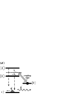
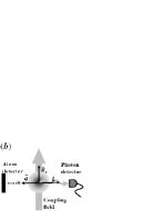
Figure 1: (a) Atomic configuration with two well–separated upper levels. The momentum entanglement can be controlled by the classical coupling field through the SGC. (b) Schematic diagram for the momentum detections. The detectors for the atom and photon are restricted in one–dimension which is perpendicular to the propagation direction of the coupling light.

Concerning the kinetic degrees of freedom, the Hamiltonian for the system depicted in Fig. 1 (a) can be written with the rotating wave approximation (RWA) as:

$$\hat{H}=\frac{(\hbar\hat{\vec{p}})^{2}}{2m}+\sum_{\vec{k}}\hbar\omega_{\vec{k}}\hat{a}^{{\dagger}}_{\vec{k}}\hat{a}_{\vec{k}}+\sum_{j=1}^{2}\hbar\omega_{jc}\hat{\sigma}_{jj}+\hbar\omega_{bc}\hat{\sigma}_{bb}$$

$$+\hbar\sum_{\vec{k}}\left[g_{1}(\vec{k})\hat{\sigma}_{c1}\hat{a}^{{\dagger}}_{\vec{k}}e^{-i\vec{k}\cdot\vec{r}}+g_{2}(\vec{k})\hat{\sigma}_{c2}\hat{a}^{{\dagger}}_{\vec{k}}e^{-i\vec{k}\cdot\vec{r}}+{\rm H.C.}\right]$$

$$+\hbar\left(\Omega_{1}e^{-i\nu_{0}t}e^{i\vec{k}_{0}\cdot\vec{r}}\hat{\sigma}_{1b}+\Omega_{2}e^{-i\nu_{0}t}e^{i\vec{k}_{0}\cdot\vec{r}}\hat{\sigma}_{2b}+{\rm H.C.}\right),$$

where $\hbar\hat{\vec{p}}$ and $\vec{r}$ denote the atomic center–of–mass momentum and position operators. $\hat{\sigma}_{\alpha\beta}$ denotes the atomic operator $|\alpha\rangle\langle\beta|$ ($\alpha,\beta=1,2,b,c$), and $\hat{a}_{\vec{k}}$ ($\hat{a}^{{\dagger}}_{\vec{k}}$) is the annihilation (creation) operator for the $k$th photonic mode with wave vector $\vec{k}$ and frequency $\omega_{\vec{k}}=ck$, where we use $\vec{k}$ to include both the momentum and polarization of the photonic mode for simplicity. $g_{j}(\vec{k})$ is the coupling coefficient for the transition $|j\rangle\rightarrow|c\rangle$ $(j=1,2)$ and $\Omega_{j}$ denotes the Rabi frequency for the coupling $|j\rangle\leftrightarrow|b\rangle$ $(j=1,2)$. For the convenience in further calculations, we may neglect the dependence on $\vec{k}$ for $g_{j}(\vec{k})$ and treat them as constants. $\nu_{0}$ and $\vec{k}_{0}$ denotes the frequency and the wave vector of the coupling light, and $\omega_{\alpha\beta}$ is used to represent the frequency difference as: $\omega_{\alpha\beta}\equiv\omega_{\alpha}-\omega_{\beta}$. As the evolution is considered in a close system, it is convenient to expand the photon–atom state in the Schrödinger picture as:

$$|\psi\rangle = \sum_{\vec{q}}\left[a_{1}(\vec{q})|\vec{q},0,1\rangle+a_{2}(\vec{q})|\vec{q},0,2\rangle+b(\vec{q})|\vec{q},0,b\rangle\right]$$ (2)

$$+ \sum_{\vec{q},\vec{k}}c(\vec{q},\vec{k})|\vec{q},\vec{k},c\rangle,$$

where the arguments in the kets denote, respectively, the wave vector of the atom, the photon, and the atomic internal state.

From the Schrödinger equation one may yield the dynamic equations for the system with the Born–Markov approximation. With the transformation to the slowly varying parts:

$$a_{1}(\vec{q}) = e^{-i[T(\vec{q})+\omega_{1c}]t}\cdot A_{1}(\vec{q}),$$ (3)

$$a_{2}(\vec{q}) = e^{-i[T(\vec{q})+\omega_{2c}]t}\cdot A_{2}(\vec{q}),$$ (4)

$$b(\vec{q}-\vec{k}_{0}) = e^{-i[T(\vec{q}-\vec{k}_{0})+\omega_{bc}]t}\cdot B(\vec{q}-\vec{k}_{0}),$$ (5)

$$c(\vec{q},\vec{k}) = e^{-i[T(\vec{q})+\omega_{\vec{k}}]t}\cdot C(\vec{q},\vec{k}),$$ (6)

where $T(\vec{p})\equiv\hbar\vec{p}^{2}/2m$ and $\Delta_{j}\equiv\omega_{jb}-\nu_{0}$ $(j=1,2)$, we yield:

$$i\frac{{\rm d}A_{1}(\vec{q})}{{\rm d}t} = \Omega_{1}e^{i\Delta_{1}t}B(\vec{q}-\vec{k}_{0})-\frac{i\gamma_{1}}{2}A_{1}(\vec{q})$$ (7)

$$- \frac{i\epsilon\sqrt{\gamma_{1}\gamma_{2}}}{2}A_{2}(\vec{q})e^{i\omega_{12}t},$$

$$i\frac{{\rm d}A_{2}(\vec{q})}{{\rm d}t} = \Omega_{2}e^{i\Delta_{2}t}B(\vec{q}-\vec{k}_{0})-\frac{i\gamma_{2}}{2}A_{2}(\vec{q})$$ (8)

$$- \frac{i\epsilon\sqrt{\gamma_{1}\gamma_{2}}}{2}A_{1}(\vec{q})e^{-i\omega_{12}t},$$

$$i\frac{{\rm d}B(\vec{q}-\vec{k}_{0})}{{\rm d}t} = \Omega_{1}^{*}e^{-i\Delta_{1}t}A_{1}(\vec{q})+\Omega_{2}^{*}e^{-i\Delta_{2}t}A_{2}(\vec{q}),$$ (9)

$$i\frac{{\rm d}C(\vec{q},\vec{k})}{{\rm d}t} = g_{1}e^{i[T(\vec{q})-T(\vec{q}+\vec{k})+\omega_{\vec{k}}-\omega_{1c}]t}\cdot A_{1}(\vec{q}+\vec{k})$$

$$+ g_{2}e^{i[T(\vec{q})-T(\vec{q}+\vec{k})+\omega_{\vec{k}}-\omega_{2c}]t}\cdot A_{2}(\vec{q}+\vec{k}),$$

where $\gamma_{1,2}$ denote the linewidthes for the two upper levels $|1\rangle$ and $|2\rangle$; and $\epsilon\equiv\vec{\mu}_{1}\cdot\vec{\mu}_{2}/|\vec{\mu}_{1}|\cdot|\vec{\mu}_{2}|$ with $\vec{\mu}_{j}$ being the dipole moment for the transition $|j\rangle\rightarrow|c\rangle$ $(j=1,2)$. As in the experiments exp , we restrict the detections for the photon and atom in one dimension, which is also perpendicular to the propagation of the coupling field, as depicted in Fig. 1 (b).

In order to have strong interference between the transitions $|1\rangle\rightarrow|c\rangle$ and $|2\rangle\rightarrow|c\rangle$, the dipoles for the transitions should be parallel or antiparallel, i.e., $\epsilon=\pm 1$ SGC theory ; SGC-induced entang ; furthermore, the dressed states produced by the coupling field should be nearly degenerate, which may be fulfilled when $\Delta_{1}/\Delta_{2}\approx-\gamma_{1}/\gamma_{2}$ SGC theory . To be consistent with these restrictions, as in some experiments SGC exp , we assume $\epsilon=1$, $\gamma_{1}=\gamma_{2}=\gamma$, $\Omega_{1}=\Omega_{2}=\Omega$; and $\Delta_{2}=-\Delta$, $\Delta_{1}=(1+\delta)\Delta$, where $\delta$ is a dimensionless small term controlled by the detuning of the coupling field. The atom is initially prepared in state $|b\rangle$ with momentum wavefunction as $G(\vec{q})\propto\exp{[-(\vec{q}/\delta_{p})^{2}]}$, where $\delta_{p}$ denotes its momentum variance.

With the above simplifications, from Eqs. (7) to (10), it is straightforward to yield the solutions for the whole system. As a result, the steady state atom–photon entangled wave function reads:

$$C(q,k,t\rightarrow\infty)\approx\chi_{0}\frac{\exp{[-(\Delta q/\eta)^{2}]}}{-\lambda_{1}/\gamma+i(\Delta q+\Delta k)}.$$ (11)

The $\Delta q$, $\Delta k$ $\eta$ and $\lambda_{1}$ are defined in the appendix, where the other related mathematical details are also given. $\chi_{0}$ is a normalization factor.

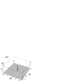
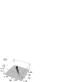
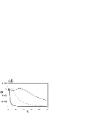
Figure 2: (a) Distribution of $|C(\Delta q,\Delta k)|^{2}$ with $\gamma=1$, $\Delta=10$, $\Omega=1$, $\delta=0.01$, $\eta$=0.001. One sees that the central peak dominates the whole function. (b) Plot of the local amplification of (a), which shows that $\Delta q$ and $\Delta k$ are highly correlated in the central peak. (c) Plot of the function $\Theta(\Omega)$ with $\Delta$ specified as 5, 15, 40, for the bold, thin and dashed lines, respectively. (d) Plot of $\Theta(\Delta)$ with $\Omega$ specified as 0.5, 3, 10, for the bold, thin and dashed lines, respectively. $\gamma=1$.

Theoretically, the entanglement of a pure state bipartite system can be completely evaluated by the Schmidt number $K$ Schmidt num , which is defined as an estimation of the number of modes that make up the Schmidt decomposition. From Eq. (11), it is found that Singlephoton ; scattering

$$K \approx 1+0.28\left[\frac{\eta}{|{\rm Re}(\lambda_{1}/\gamma)|}-1\right],$$ (12)

$$\approx\frac{0.28\eta}{|\Theta(\Delta/\gamma,\Omega/\gamma)|\delta^{2}},$$

where the function $\Theta(\Delta/\gamma,\Omega/\gamma)$ is defined in the appendix and depicted in Figs. 2 (c) and (d). With respect to the realistic detections in experiment exp , however, the degree of entanglement is better to be characterized by the ratio ($R$) of the unconditional and conditional variances in the momentum detections 3-D spontaneous ; GR ; photoionization , i.e.:

$$R\equiv\delta q^{{\rm single}}/\delta q^{{\rm coin}},$$ (13)

$$\delta q^{{\rm single}}\equiv\langle\hat{p}^{2}\rangle_{{\rm single}}-\langle\hat{p}\rangle_{{\rm single}}^{2},$$ (14)

$$\delta q^{{\rm coin}}\equiv\langle\hat{p}^{2}\rangle_{{\rm coin}}-\langle\hat{p}\rangle_{{\rm coin}}^{2},$$ (15)

where $\delta q^{{\rm single}}$ is defined as the variance of the atomic momentum with single–particle detection, and $\delta q^{{\rm coin}}$ denotes the variance obtained by the coincidence detection on both the atom and the photon. From Eqs. (11) and (13), we yield:

$$R\approx\frac{\eta}{1.6|{\rm Re}(\lambda_{1}/\gamma)|}=\frac{\eta}{1.6|\Theta(\Delta/\gamma,\Omega/\gamma)|\delta^{2}}\approx 2.2K,$$ (16)

where one sees that the Schmidt number $K$ can therefore be obtained experimentally by measuring the $R$ ratio exp .

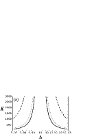
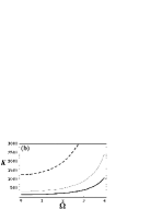
Figure 3: Relations between the Schmidt number $K$ and the coupling field with $\gamma=1$, $\omega_{12}=20$, $\eta=0.001$. (a) The bold, thin and dashed lines are plotted with $\Omega=0.1$, $\Omega=2$ and $\Omega=4$, respectively. (b) The bold, thin and dashed lines are plotted with $\Delta=9.97$, $\Delta=9.98$ and $\Delta=9.99$, respectively.

With Eq. (12) or (16), one sees that the entanglement is most sensitive with the relative detuning $\delta$, therefore with the frequency of the coupling field. With the relation $\omega_{12}=\Delta_{1}-\Delta_{2}=(2+\delta)\Delta$, we plot in Fig. 3 the degree of entanglement $K$ with respect to the detuning $\Delta=\nu_{0}-\omega_{2b}$ and Rabi frequency $\Omega$ of the coupling field. From Fig. 3 and Eq. (12), one sees that the entanglement can be effectively enhanced by controlling the coupling field, and when $\nu_{0}\rightarrow\omega_{2b}+\omega_{12}/2$, we have $K\rightarrow\infty$.

Different to some previous works scattering ; GR , the superhigh entanglement produced with this scheme is due to the atomic spontaneously generated coherence (SGC) SGC theory ; SGC-induced entang . With parallel dipoles ($\epsilon=1$), the photon emitted along the two transition pathes $|1\rangle\rightarrow|c\rangle$ and $|2\rangle\rightarrow|c\rangle$ will interfere and modify the momentum entanglement with the recoiled atom as a result. In recent studies, it is found that, with nearly degenerate upper levels and proper atomic coherence, the atom with SGC may exhibit anomalous enhancement of momentum entanglement in the spontaneous emission process SGC-induced entang . In this scheme, however, it is shown that, even with well–separated upper levels and realistic conditions SGC exp , the entanglement could also be highly increased with the quantum interference which can be controlled by a classical light field. Therefore, the proposed scheme can most probably be used to produce highly entangled atom–photon pairs in realistic applications.

III disentanglement

As in the preceding section, to study the generation of momentum entanglement Singlephoton ; scattering ; GR ; 3-D spontaneous , it is usually convenient to assume the entangled system to be a close pure state system. However, in a realistic environment with $T\gg 0{\rm K}$, the interaction with environment will make the entangled system into a mixed state, and, as a result, cause the disentanglement. Actually, only when the disentangling process is much slower than the generation of entanglement, the entangled system can well be approximated by a pure state. With these considerations, it is then possible to give out an upper bound for the entanglement that could be produced reliably in the environment.

Concerning the momentum entanglement, the disentanglement is caused by the momenta exchange with the environment which may be composed of background atoms and photons. Theoretically, the influence from the background atoms can be eliminated by using a high vacuum system; therefore, in order to study the unavoidable disentanglement, we can simplify the environment as a heatbath of background photons, coupled only to the entangled atom, as shown in Fig. 4 (a). In order to give a general analysis for this incoherent process, the atom is simplified as a two–level system with resonant frequency $\omega_{a}$, then the Hamiltonian of the total system under RWA is:

$$\hat{H}_{{\rm tot}} = \hat{H}_{{\rm S}}+\hat{H}_{{\rm B}}+\hat{H}_{{\rm I}},$$ (17)

$$\hat{H}_{{\rm S}} = \frac{(\hbar\hat{p})^{2}}{2m}+\hbar\omega_{a}\hat{\sigma}_{22}+\sum_{k}\hbar\omega_{k}\hat{b}^{{\dagger}}_{k}\hat{b}_{k},$$ (18)

$$\hat{H}_{{\rm B}} = \sum_{k}\hbar\omega_{k}\hat{a}^{{\dagger}}_{k}\hat{a}_{k},$$ (19)

$$\hat{H}_{{\rm I}} = \hbar\sum_{k}\left[g(k)\hat{\sigma}_{12}\hat{a}^{{\dagger}}_{k}e^{-ikr}+{\rm H.C.}\right],$$ (20)

where $\hat{H}_{{\rm S}}$, $\hat{H}_{{\rm B}}$ and $\hat{H}_{{\rm I}}$ denote the Hamiltonians for the system (the entangled atom–photon pair), the heatbath and the interaction between them, respectively. $\hat{b}_{k}$ ($\hat{b}^{{\dagger}}_{k}$) is the annihilation (creation) operator for the entangled single–photon in its $k$th mode, whereas $\hat{a}_{k}$ and $\hat{a}^{{\dagger}}_{k}$ are those for the photons in the heatbath.

It is known that the density matrix of the total system $\rho_{{\rm tot}}$ obeys the Liouville equation:

$$\dot{\rho}_{\rm tot}=\mathcal{L}_{{\rm tot}}(\rho_{{\rm tot}})=(\mathcal{L}_{{\rm S}}+\mathcal{L}_{{\rm B}}+\mathcal{L}_{{\rm I}})\rho_{{\rm tot}},$$ (21)

where the superoperators $\mathcal{L}_{{\rm tot}}$, $\mathcal{L}_{{\rm S}}$, $\mathcal{L}_{{\rm B}}$ and $\mathcal{L}_{{\rm I}}$ are defined as: $\mathcal{L}_{{\rm tot}}(*)\equiv-\frac{i}{\hbar}[\hat{H}_{{\rm tot}},*]$, etc.. In order to reveal the dynamic evolution for the entangled system, we should adiabatically eliminate the heatbath terms from Eq. (21) to obtain the master equation for the entangled system.

To proceed, we define the reduced density matrix for the system as $\rho\equiv{\rm Tr_{B}}(\rho_{{\rm tot}})$ and a “projection state” as $v\equiv{\rm Tr_{B}}(\rho_{{\rm tot}})\otimes\rho_{{\rm B}}$, where the trace “${\rm Tr_{B}}$” is taken over the heatbath space and $\rho_{{\rm B}}$ denotes the initial state of the heatbath. As the coupling is weak, from Eq. (21), we yield the equation for the projection state as:

$$\dot{v}=\mathcal{L}_{{\rm S}}v-i\rho_{{\rm B}}\otimes{\rm Tr_{B}}\left(\mathcal{L}_{{\rm I}}\int^{\infty}_{0}{\rm d}\tau\left[\sum_{k}g(k)\hat{a}^{{\dagger}}_{k}e^{-iw_{k}\tau}\Lambda(\tau)+{\rm H.C.}\ ,\ \rho\otimes\rho_{{\rm B}}\right]\right),$$ (22)

where the Markov approximation and the nonrelativistic approximation $\hbar k/mc\ll 1$ are used, and $\Lambda(\tau)\equiv e^{-i\hat{H}_{{\rm S}}\tau/\hbar}\hat{\sigma}_{12}e^{-ikr}e^{i\hat{H}_{{\rm S}}\tau/\hbar}$.

From Eq. (22), we yield the master equation with the Lindblad form Lindblad as:

$$\dot{\rho} = -\frac{i}{\hbar}[\hat{H}_{{\rm S}},\rho]-\Gamma_{a}\left[D(\hat{\sigma}_{11}\rho+\rho\hat{\sigma}_{11})+(1+D)(\hat{\sigma}_{22}\rho+\rho\hat{\sigma}_{22})\right]+(1+D)\Gamma_{a}\left[\hat{\sigma}_{12}e^{-ik_{a}r}\rho\hat{\sigma}_{21}e^{ik_{a}r}+\hat{\sigma}_{12}e^{ik_{a}r}\rho\hat{\sigma}_{21}e^{-ik_{a}r}\right]$$ (23)

$$+ D\Gamma_{a}\left[\hat{\sigma}_{21}e^{ik_{a}r}\rho\hat{\sigma}_{12}e^{-ik_{a}r}+\hat{\sigma}_{21}e^{-ik_{a}r}\rho\hat{\sigma}_{12}e^{ik_{a}r}\right],$$

where $D\equiv{\rm Tr_{B}}(\hat{a}^{{\dagger}}_{k_{a}}\hat{a}_{k_{a}}\rho_{{\rm B}})$ is the average number of the resonant photons in the heatbath; the atomic linewidth is given as $\Gamma_{a}\equiv\sum_{k}2\pi|g(k)|^{2}\delta(\omega-\omega_{a})$. It is natural to assume that the heatbath is initially in the thermal equilibrium, i.e., $\rho_{{\rm B}}=e^{-\hat{H}_{{\rm B}}/k_{B}T}/{\rm Tr_{B}}(e^{-\hat{H}_{{\rm B}}/k_{B}T})$, then we have $D=1/(e^{\hbar\omega_{a}/k_{B}T}-1)$, where $T$ is the temperature of the heatbath.

The master equation, Eq. (23), describes the process of disentanglement, where the entangled system is now in a mixed state due to the interaction with the heatbath. Theoretically, the entanglement of a mixed bipartite system can be evaluated with the “entanglement of formation”ent of formation . However, in order to base our analysis on direct experimental test exp , we use the defined $R$ ratio [cf. Eq. (13)] as the evaluation of the entanglement.

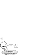
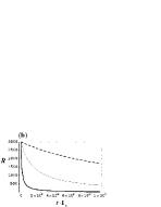
Figure 4: (a) Schematic diagram of the disentanglement. The atom is treated as a two–level system and the environment is simplified as a heatbath of photons which is coupled to the atom through momenta exchange. (b) $R(t)$ is plotted with $\delta q^{{\rm single}}_{0}=16k_{a}^{2}$ and $R_{0}$=3000. The temperature of the environment is specified as $T=300{\rm\ K}$ for the bold line, $T=270{\rm\ K}$ for the thin line and $T=250{\rm\ K}$ for the dashed line.

As in Eqs. (14) and (15), the momentum variance of the single–particle (the atom) measurement is calculated as:

$$\delta q^{{\rm single}}={\rm Tr}(\hat{p}^{2}\rho)-[{\rm Tr}(\hat{p}\rho)]^{2},$$ (24)

while that of the coincidence measurement is:

$$\delta q^{{\rm coin}} = \frac{\sum_{i=1}^{2}\int{\rm d}q\ q^{2}\rho(q,k_{0},i,q,k_{0},i)}{\sum_{i=1}^{2}\int{\rm d}q\ \rho(q,k_{0},i,q,k_{0},i)}$$ (25)

$$- \left(\frac{\sum_{i=1}^{2}\int{\rm d}q\ q\rho(q,k_{0},i,q,k_{0},i)}{\sum_{i=1}^{2}\int{\rm d}q\ \rho(q,k_{0},i,q,k_{0},i)}\right)^{2},$$

where $\rho(q,k,i,q^{\prime},k^{\prime},i^{\prime})$ denotes the matrix element $\langle q,k,i|\rho|q^{\prime},k^{\prime},i^{\prime}\rangle$, and the photon is assumed to be detected with some momentum $k_{0}$.

With Eqs. (23) to (25), it is straightforward to get:

$$R(t)=R_{0}\cdot\frac{\delta q^{{\rm single}}_{0}/4Dk_{a}^{2}+\Gamma_{a}t}{\delta q^{{\rm single}}_{0}/4Dk_{a}^{2}+R_{0}\Gamma_{a}t},$$ (26)

where $R_{0}$ and $\delta q^{{\rm single}}_{0}$ are defined as their initial values, $R_{0}\equiv R(t=0)$ and $\delta q^{{\rm single}}_{0}\equiv\delta q^{{\rm single}}(t=0)$. It can be seen from Fig. 4 (b) that, $R(t)$ decreases monotonously with time, therefore, the characteristic time scale $\Delta t_{{\rm dis}}$ for the disentanglement can be defined as $R(t=\Delta t_{{\rm dis}})=\frac{1}{2}R_{0}$. As $R_{0}\gg 1$, we yield:

$$\Delta t_{{\rm dis}}\approx\frac{\delta q^{{\rm single}}_{0}}{4DR_{0}k_{a}^{2}\Gamma_{a}}.$$ (27)

From Eq. (27), one sees that the “disentangling time” $\Delta t_{{\rm dis}}$ is inversely proportional to the average number of the resonant photons in the heatbath [$D(\omega_{a})$]. Therefore, by decreasing the temperature of the environment it is possible to significantly increase $\Delta t_{{\rm dis}}$ and then make the entangled system quite robust in the environment. However, as the temperature can never reach absolute zero, this kind of disentanglement is “unavoidable”. Furthermore, as in Eq. (27), the disentangling time is also dependent on the initial entanglement, i.e., $\Delta t_{{\rm dis}}\propto 1/R_{0}$, which indicates that, the better entangled system is more fragile in the environment. Since $\Delta t_{{\rm dis}}\rightarrow 0$ when $R_{0}\rightarrow\infty$, the ideal continuous EPR state EPR can never be reached in a realistic environment in this sense.

The physical meaning for the dependence on $k_{a}$ and $\Gamma_{a}$ in Eq. (27) is apparent: with larger energy and shorter lifetime for the transitions, the environment will exchange more momenta with the entangled atom per unit time, and as a result, accelerate the disentanglement. When temperature is low, the denominator in Eq. (27) has a sharp peak for the coupled frequency $\omega_{a}$, which ensures the two–level approximation reasonable for our treatment.

As stated at the beginning of this section, the entanglement generated with Eqs. (12) and (16) is applicable only if the disentangling time is much longer than the time scale for producing the entanglement, i.e., $\Delta t_{{\rm dis}}\gg\Delta t_{{\rm ent}}$. Therefore, with the Eqs. (27) and (A8), we yield the inequality:

$$R_{0}\ll 0.2\sqrt{\frac{\hbar k_{1c}\delta_{p}^{3}}{Dmk_{a}^{2}\Gamma_{a}}},$$ (28)

which gives an upper bound for the entanglement that can be produced in realistic environment with this scheme.

As in some reported experiments SGC exp , the atomic configuration with SGC as in Fig. 1 (a) can be realized by sodium dimers. With the experimental conditions $\gamma\sim 10^{-7}\omega_{1c}$, $\omega_{12}\sim 10\gamma$, $\Omega\sim\gamma$, when the coupling field is tuned to $\Delta\sim\omega_{12}/2\sim 5\gamma$ with $\delta=10^{-2}$, from Eq. (A8), we have $\Delta t_{{\rm ent}}\sim 1{\rm ms}$. Take the time–of–flight into account scattering , the initial momentum variance can be prepared as $\hbar\delta_{p}/m=1{\rm m/s}$, and then from Eq. (16) we obtain a superhigh degree of entanglement as $R\approx 4600$ and $K\approx 2100$. To consider the disentanglement, we take $\omega_{a}=5\times 10^{14}{\rm Hz}$ and $\Gamma_{a}=10^{7}{\rm Hz}$ for estimations. With the environment temperature $T=150{\rm K}$, from Eq. (27), we have $D\sim 10^{-11}$ and $\Delta t_{{\rm dis}}\sim 10^{4}{\rm s}$. One sees that the relation $\Delta t_{{\rm ent}}\ll\Delta t_{{\rm dis}}$ can be well fulfilled. Therefore, under these conditions, the robust highly entangled atom–photon pairs can be steadily produced in the environment. Actually, from Eq. (28), we have an upper bound as $R\ll 10^{7}$, which implies a strong ability of producing entanglement with this scheme. On the other hand, if the environment is at a high temperature, e.g., $T=400{\rm\ K}$, the disentanglement will be strongly enhanced and we now have $\Delta t_{{\rm ent}}\sim\Delta t_{{\rm dis}}$. With direct detections exp , it is then possible to observe all these phenomena in experiment.

IV conclusion

In this paper, we demonstrate a novel scheme to produce superhigh momentum entanglement between a single atom and a single photon with the atomic SGC SGC-induced entang . Under certain experimental conditions SGC exp , we show that the entanglement can be effectively controlled by the classical coupling field and may be very robust against the disentanglement due to the environment. As we analyze the two physical processes separately and both from the first principle, most of our conclusions can directly apply to the previous models 3-D spontaneous ; GR ; scattering ; Singlephoton .

To give a better upper bound than Eq. (28), one may consider the generation of entanglement together with the disentanglement at the same time, which is also necessary to analyze the system when $\Delta t_{{\rm ent}}\sim\Delta t_{{\rm dis}}$ rigorously. However, this method is more complicated to be generalized and will not change our above conclusions qualitatively. We plan to give the details of this method elsewhere in a future work.

This work is supported by the National Natural Science Foundation of China (Grant No. 10474004), and DAAD exchange program: D/05/06972 Projektbezogener Personenaustausch mit China (Germany/China Joint Research Program).

Appendix: steady solutions of equations (7) to (10)

In order to obtain Eq. (11), we define a matrix $M$ as:

$$M=\left(\begin{array}[]{ccc}\frac{\gamma_{1}}{2}+i\Delta_{1},&\frac{\epsilon\sqrt{\gamma_{1}\gamma_{2}}}{2},&i\Omega_{1}\\ \frac{\epsilon\sqrt{\gamma_{1}\gamma_{2}}}{2},&\frac{\gamma_{2}}{2}+i\Delta_{2},&i\Omega_{2}\\ i\Omega_{1}^{*},&i\Omega_{2}^{*},&0\end{array}\right),$$ (A1)

its eigenvalues and eigenvectors are denoted, respectively, as $\lambda_{j}$ and $(\alpha_{j},\beta_{j},\zeta_{j})^{{\rm T}}$ with $j=1,2,3$. Then from Eqs. (7) to (10), the steady state solution of the entangled wave function can be written as:

$$C(\vec{q},\vec{k},t\rightarrow\infty)=$$ (A2)

$$\sum_{j=1}^{3}\frac{i(g_{1}\alpha_{j}+g_{2}\beta_{j})p_{j}G(\vec{q}+\vec{k}-\vec{k}_{0})}{-\lambda_{j}+i\left[T(\vec{q})-T(\vec{q}+\vec{k})+\omega_{\vec{k}}-(\omega_{bc}+\nu_{0})\right]},$$

where $p_{j}$ is determined by the initial conditions, and when the atom is initially in $|b\rangle$, the restrictions are:

$$\sum_{j=1}^{3}p_{j}\alpha_{j}=0,\ \ \sum_{j=1}^{3}p_{j}\beta_{j}=0,\ \ \sum_{j=1}^{3}p_{j}\zeta_{j}=1.$$ (A3)

As the detection is restricted in one dimension, the solution can be simplified as:

$$C(q,k) \propto\sum_{j=1}^{3}\frac{(g_{1}\alpha_{j}+g_{2}\beta_{j})p_{j}e^{-(\Delta q/\eta)^{2}}}{-\lambda_{j}/\gamma_{2}+i(\Delta q+\Delta k)},$$ (A4)

$$\equiv\sum_{j=1}^{3}L_{j}(\Delta q,\Delta k),$$ (A5)

where the effective wave vectors are defined as:

$$\Delta q \equiv\frac{\hbar(\omega_{bc}+\nu_{0})}{mc\gamma_{2}}(q-\frac{\omega_{bc}+\nu_{0}}{c}),$$ (A6)

$$\Delta k \equiv\frac{ck-(\omega_{bc}+\nu_{0})}{\gamma_{2}},$$ (A7)

and $\eta\equiv\hbar(\omega_{bc}+\nu_{0})\delta_{p}/m\gamma_{2}c$. We use $L_{1,2,3}(\Delta q,\Delta k)$ here to denote the three different terms that make up the summation in Eq. (A4). From Eq. (A4), it can be proved that:

$$\int{\rm d}\Delta q{\rm d}\Delta k|L_{2,3}(\Delta q,\Delta k)|^{2}=o(\Omega^{2}/\gamma^{2})\ \ {\rm when}\ \Omega\rightarrow 0,$$

which indicates that the $L_{1}(\Delta q,\Delta k)$ dominates the summation when the coupling field is weak, as shown in Figs. 2 (a) and 2 (b); therefore, Eq. (A4) can be well approximated by the single–peak function as in Eq. (11).

To give further analysis for the entanglement, from Eq. (A1), we yield ${\rm Re}(\lambda_{1}/\gamma)\approx\Theta(\Delta/\gamma,\Omega/\gamma)\delta^{2}$, where the value of $\Theta(\Delta/\gamma,\Omega/\gamma)$ is of order $0.1$ or smaller as shown in Figs. 2 (c) and (d). Moreover, the time scale for producing the entanglement can be characterized as: $\Delta t_{{\rm ent}}=1/|{\rm Re}(\lambda_{1})|=1/\gamma|\Theta|\delta^{2}$, with Eq. (16), it may be written as:

$$\Delta t_{{\rm ent}}\approx\frac{1.6R}{\eta\gamma}.$$ (A8)

References

(1) A. Einstein, B. Podolsky, N. Rosen, Phys. Rev. 47,
777 (1935); J. C. Howell et. al., Phys. Rev. Lett.
92, 210403 (2004).
(2) S. L. Braunstein and P. V. Loock, Rev. Mod. Phys.
77, 513 (2005).
(3) K. W. Chan, C. K. Law, and J. H. Eberly,
Phys. Rev. Lett. 88, 100402 (2002).
(4) K. W. Chan et. al., Phys. Rev. A 68,
022110 (2003); J. H. Eberly, K. W. Chan and C. K. Law, Phil.
Trans. R. Soc. Lond. A 361, 1519 (2003).
(5) M. V. Fedorov et. al., Phys. Rev.
A 72, 032110 (2005).
(6) R. Guo and H. Guo, Phys. Rev. A 73, 012103
(2006).
(7) M. V. Fedorov et al., Phys. Rev. A
69, 052117 (2004).
(8) M. D. Reid and P. D. Drummond, Phys. Rev. Lett. 60,
2731 (1988); Michael S. Chapman et al., Phys. Rev. Lett.
75, 3783 (1995); Christian Kurtsiefer et al.,
Phys. Rev. A 55, R2539 (1997).
(9)H. R. Xia, C. Y. Ye, and S. Y. Zhu, Phys. Rev. Lett. 77,
1032 (1996).
(10)S. Y. Zhu and M. O. Scully, Phys. Rev. Lett 76, 388
(1996).
(11)arXiv: R. Guo and H. Guo,
quant–ph/0701018v2; S. Y. Zhu, R. C. F. Chan and C. P. Lee, Phys.
Rev. A 52, 710 (1995).
(12) R. Grobe et al., J. Phys. B 27,
L503 (1994); S. Parker et al., Phys. Rev. A 61,
032305 (2000); C. K. Law, I. A. Walmsley, and J. H. Eberly, Phys.
Rev. Lett. 84, 5304 (2000); W. C. Liu, S. L. Haan, R.
Grobe, J. H. Eberly, Phys. Rev. Lett. 83, 520 (1999).
(13) G. Lindblad, Comm. Math. Phys. 48, 119
(1976).
(14)C. H. Bennett, D. P. DiVincenzo, J. A.
Smolin and W. K. Wootters, Phys. Rev. A 54, 3824 (1996).