Path integrals and wavepacket evolution for damped mechanical systems

Abstract

Damped mechanical systems with various forms of damping are quantized using the path integral formalism. In particular, we obtain the path integral kernel for the linearly damped harmonic oscillator and a particle in a uniform gravitational field with linearly or quadratically damped motion. In each case, we study the evolution of Gaussian wave packets and discuss the characteristic features that help us distinguish between different types of damping. For quadratic damping, we show that the action and equation of motion of such a system has a connection with the zero dimensional version of a currently popular scalar field theory. Furthermore we demonstrate that the equation of motion (for quadratic damping) can be identified as a geodesic equation in a fictitious two-dimensional space.

I Introduction

The presence of damping in a mechanical system is a natural occurrence. For example, consider a particle falling through a fluid under gravity. The form of the damping force depends on the value of the Reynolds number ${\rm Re}=\rho\ell v/\eta$, where $\rho$ is the fluid density, $\eta$ the viscosity coefficient, $\ell$ the characteristic length scale, and $v$ the speed of the particle in the fluid. For ${\rm Re}<1$ we may assume linear damping and for ${10}^{3}<{\rm Re}<2\times{10}^{5}$ it is more natural to assume that the damping is quadratic in the velocity.timmerman The assumption of a nonlinear damping term makes the equation of motion nonlinear and more difficult to handle in general. Several classical mechanical systems with linear as well as nonlinear damping are exactly solvable.mechanics

In contrast, the quantum mechanics of damped mechanical systems is not as easy to understand. Usually we write down Schrödinger’s equation for a given potential and obtain the energy eigenvalues and eigenfunctions either exactly or by approximation methods. This procedure does not work for damped systems because of either the explicit time dependence or the complicated form of the Lagrangian and hence the Hamiltonian.

The primary goals of this article are to show that Lagrangians can be constructed for simple damped systems, to use these Lagrangians to construct the path integral kernels for damped systems, and to study the wavepacket evolution using these kernels. Our results supplement the existing literature on exact path integrals for mechanical systems.

Our examples include the damped simple harmonic oscillator and the freely falling particle in a uniform gravitational field in the presence of linear/ or quadratic damping. Earlier work on the quantization of damped systems can be found in Refs. milburn, ; herrera, ; yurke, using a variety of techniques such as variational methods, the Fokker-Planck equation, and canonical quantization. Path integral techniques have been used by several authors (see for example, Refs. holstein1, ; chaos, ; holstein2, ; cohen, ; moriconi, ; poon, ; thornber, ; laurent, ). A comprehensive and up-to-date analysis on various aspects of path integrals (with associated references) is available in Ref. kleinert, .

In Sec. II we outline the path integral formalism, which we shall use extensively. Then in Sec. III.1 we consider the damped harmonic oscillator and discuss the construction of the kernel for the under-damped case in detail. As a second example, we consider in Sec. III.2 a particle falling under gravity in the presence of a linear damping force. In Sec. IV we focus on quadratic damping in an analogous way. In all these systems we study wavepacket evolution and show how the dispersion of the packet provides us with a way of distinguishing between the magnitude as well as various forms of the damping force. As an aside (and a motivation for the reader who wishes to find a taste of advanced physics from an elementary standpoint) we connect the quadratic damping scenario with a recently studied field theory. In the same spirit, we also illustrate how quadratically damped motion can be viewed as a geodesic motion in a fictitious two-dimensional space. In Sec. V we conclude with a summary of our results.

II Path integral formalism

Before we begin our discussion of the path integral treatment of damped mechanical systems we give some results that we will use in our analyses. For readers interested in the details of this formalism there are several good references including Refs. feyn1, ; kleinert, ; narlikar, ; sakurai, .

For a particle propagating from the initial point $(x_{i},t_{i})$ to the final point $(x_{f},t_{f})$ the transition amplitude is given by the integral over all possible paths connecting the initial and the final points:

$$K(x_{f},t_{f};x_{i},t_{i})=\!\int_{(x_{i},t_{i})}^{(x_{f},t_{f})}\!e^{iS[{\cal L}(x,\dot{x},t)]/\hbar}\,{\cal D}x,$$ (1)

where $S$ and $\cal{L}$ denote, respectively, the classical action and the Lagrangian of the particle. The transition amplitude $K(x_{f},t_{f};x_{i},t_{i})$ is called the propagator. It can be shown that for a general quadratic Lagrangian the form of the propagator reduces tonarlikar

$$K(x_{f},t_{f};x_{i},t_{i})=\phi(t_{f},t_{i})e^{iS[{\cal L}(x_{\rm cl},\dot{x}_{\rm cl},t)]/\hbar},$$ (2)

where the factor $\phi(t_{f},t_{i})$ is a function of the initial and the final time. The subscript “cl” refers to classical solution of the equation of motion.

An important property of the propagator, known as transitivity, is obtained by considering an instant of time $t$ such that $t_{f}>t>t_{i}$

$$K(x_{f},t_{f};x_{i},t_{i})=\!\int\!dx\,K(x_{f},t_{f};x,t)K(x,t;x_{i},t_{i}).$$ (3)

We will make use of Eqs. (2) and (3) in our subsequent discussion.

III Path integral formulation of linearly damped systems

We now illustrate the method of path integrals outlined in Sec. II by applying it to some simple damped mechanical systems. We will assume that the motion takes place between fixed initial and final points and calculate the kernel for the systems. The kernel will then be used to study the evolution of a Gaussian wavepacket.

III.1 Linearly Damped Harmonic Oscillator

The equation of motion of a linearly damped harmonic oscillator is $m\ddot{x}+\beta\dot{x}+m{\omega_{0}}^{2}x=0$, where $m$ is the mass of the particle, $\beta$ is the damping coefficient, and $\omega_{0}$ is the frequency of its oscillations for $\beta=0$. The general solution of the equation of motion for the over-damped (OD), critically damped (CD), and under-damped (UD) cases are shown in Table 1, where $\Lambda=\beta/m$, [xx better to write $\lambda$ instead xx] $\gamma^{2}=\big{(}\frac{\Lambda^{2}}{4}-{\omega_{0}}^{2}\big{)}=-\omega^{2}$, and $T=t_{f}-t_{i}$. We use the boundary conditions $x(t_{i})=x_{i}$ and $x(t_{f})=x_{f}$ to evaluate the integration constants $A$ and $B$ (see Table I).

To construct the kernel we first need to know the Lagrangian, which is given by:

$${\cal L}=\Big{(}\frac{1}{2}m\dot{x}^{2}-\frac{1}{2}m{\omega_{0}}^{2}x^{2}\Big{)}e^{\Lambda t}.$$ (4)

Note that the Lagrangian is explicitly time dependent. There are ways of choosing new coordinates so that the Lagrangian in Eq. (4) becomes time-independent.smith It is easy to check that this Lagrangian reproduces the correct classical equation of motion for the damped harmonic oscillator. Several authors have looked at the path integral kernel for this Lagrangian. pidamped1 ; pidamped2 A reasonably up-to-date review covering various aspects is available in Ref. pidampedrev, . We now write down the kernel for the under-damped case and then investigate the wavepacket evolution. The results for the other two cases are given in Tables 2 and 3.

The classical action is evaluated by substituting the solution for the under-damped case given in Table 1 into Eq. (4) and integrating it over the time interval $[t_{i},t_{f}]$. The result is

$$S=\frac{m\omega}{2\sin{\omega T}}\big{[}(x_{i}^{2}e^{\Lambda t_{i}}+x_{f}^{2}e^{\Lambda t_{f}})\cos\omega T-2x_{i}x_{f}e^{\Lambda(t_{i}+t_{f})/2}\big{]}+\frac{m\Lambda}{4}(x_{i}^{2}e^{\Lambda t_{i}}-x_{f}^{2}e^{\Lambda t_{f}}).$$ (5)

The effect of damping appears in Eq. (5) through the presence of $\Lambda$. In particular, the second term is entirely due to damping effects. It is interesting that if we use scaled coordinates $\overline{x}_{i}=x_{i}e^{\Lambda t_{i}/2}$ and $\overline{x}_{f}=x_{f}e^{\Lambda t_{f}/2}$, we can rewrite the first term as a purely simple harmonic oscillator contribution.

Because the Lagrangian is quadratic, the kernel is of the form given in Eq. (2). We make use of the transitivity of the kernel, that is, Eq. (3) to calculate $\phi(t_{f},t_{i})$. After some algebra, we find:

$$\phi(t_{f},t_{i})=\phi(t_{f},t)\phi(t,t_{i})\sqrt{\frac{2\pi i\hbar}{m\omega e^{\Lambda t}\big{(}\frac{\cos\omega(t_{f}-t)}{\sin\omega(t_{f}-t)}+\frac{\cos\omega(t-t_{i})}{\sin\omega(t-t_{i})}\big{)}}},$$ (6)

which leads to

$$\phi(t_{f},t_{i})=\sqrt{\frac{m\omega e^{\Lambda(t_{i}+t_{f})/2}}{2\pi i\hbar\sin{\omega T}}}.$$ (7)

The complete kernel turns out to be

$$K(x_{f},t_{f};x_{i},t_{i})=\sqrt{\frac{m\omega e^{\Lambda(t_{i}+t_{f})/2}}{2\pi i\hbar\sin{\omega T}}}e^{\frac{i}{\hbar}S},$$ (8)

where $S$ is given by Eq. (5).

To determine how a Gaussian wavepacket evolves for this kernel, we begin with the initial ($t_{i}=0$) profile of the packet:

$$\psi(x_{i},0)=\Big{(}\frac{1}{2\pi{\sigma_{0}}^{2}}\Big{)}^{1/4}e^{-(x_{i}-a)^{2}/4{\sigma_{0}}^{2}},$$ (9)

where ${\sigma_{0}}^{2}$ is the variance of the Gaussian wavepacket, which is a measure of its width. Without any loss of generality we choose the wavepacket to be peaked at $x_{i}=a$ at $t_{i}=0$. The wavepacket at a later time $t$ is related to the wavepacket at $t_{i}=0$ by

$$\psi(x_{f},t)=\!\int_{-\infty}^{\infty}K(x_{f},t;x_{i},0)\psi(x_{i},0)\,dx_{i}.$$ (10)

After some simplifications, we find

$$|\psi(x_{f},t)|^{2} =\frac{1}{\sqrt{2\pi{\sigma_{t}}^{2}}}\exp\Big{[}\frac{-\big{[}x_{f}-ae^{-\Lambda t/2}\big{(}\cos\omega t+\frac{\Lambda}{2\omega}\sin\omega t\big{)}\big{]}^{2}}{2{\sigma_{t}}^{2}}\Big{]},$$ (11)

$${\sigma_{t}}^{2} ={\sigma_{0}}^{2}e^{-\Lambda t}\Big{[}\big{(}\cos\omega t+\frac{\Lambda}{2\omega}\sin\omega t\big{)}^{2}+\big{(}\frac{\hbar\sin\omega t}{2m\omega{\sigma_{0}}^{2}}\big{)}^{2}\Big{]}.$$ (12)

From Eq. (11) we see that at any time $t$ the wavepacket is peaked at

$$x_{f}=ae^{-\Lambda t/2}\Big{(}\cos\omega t+\frac{\Lambda}{2\omega}\sin\omega t\Big{)}.$$ (13)

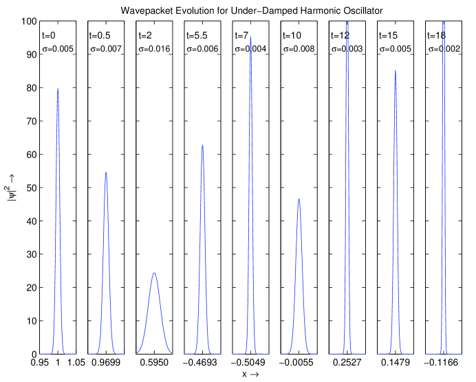
Figure 1: Evolution of wavepacket in a harmonic oscillator potential with linear damping for the parameters $\Lambda=0.2$, $\omega_{0}=0.5$, and $a=1.0$.

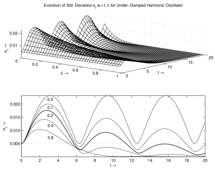
Figure 2: Variation of $\sigma_{t}$ with $t$ and $\Lambda$ for UD case [Eq. (12)]. The value of $\Lambda$ for each curve is shown just below the corresponding curve.

The wavepacket evolution is shown in Fig. 1, and the dependence of the standard deviation $\sigma_{t}$ on $t$ and $\Lambda$ is shown in Fig. 2. From Fig. 1, we notice that the width of the wavepacket pulsates and at various times it becomes less than the initial value $\sigma_{0}$. From Fig. 2 we see that $\sigma_{t}$ shows the same behavior and after $t\sim 11$ remains less than $\sigma_{0}$ for $\Lambda=0.2$ and $\omega_{0}=0.5$ (bold line). We see similar behavior for $\sigma_{t}$ for different values of $\Lambda$. The oscillations are less prominent for higher values of $\Lambda$. This behavior is seen for the critically and over-damped cases. From theoretical considerations, we expect that the under-damped case exhibits less prominent oscillations as $\Lambda\to 2\omega_{0}$. We also note that for $\Lambda=0$, $\sigma_{t}$ oscillates between $\sigma_{0}$ and $\sigma_{\max}>\sigma_{0}$ (as is well known), but as the damping coefficient becomes nonzero, the variance drops below $\sigma_{0}$ at some time and goes to zero. This behavior coincides with the wavepacket’s peak tending towards $x=0$. Thus, we conclude that the damping leads to localization of the particle around the minimum of the potential at $x=0$.

The expectation value of $x$ is

$$\langle{x}\rangle=\!\int_{-\infty}^{\infty}\!x|\psi|^{2}dx=ae^{-\Lambda t/2}\Big{(}\cos\omega t+\frac{\Lambda}{2\omega}\sin\omega t\Big{)}.$$ (14)

This result is the same as Eq. (13) and $x(t)$ for the UD case in Table 1 if $A$ and $B$ are evaluated using the initial conditions $x(0)=a$ and $\dot{x}(0)=0$. That is, the peak of the wavepacket (corresponding to the maximum probability of finding the particle) follows the classical trajectory as expected.

III.2 Uniform Gravitational Field with Linear Damping

Consider a particle of mass $m$ in a uniform gravitational field with a damping force proportional to its speed. This damping is an example of Stokes’ law. The equation of motion of the particle is $m\ddot{x}+\beta\dot{x}=mg$, where $\beta$ is the damping coefficient and $g$ the acceleration due to gravity. Recall that there is a terminal velocity, which the particle attains asymptotically. The general solution of the equation of motion is

$$x(t)=A+Be^{-\Lambda t}+\frac{g}{\Lambda}t,$$ (15)

where $\Lambda=\beta/m$, and $A$ and $B$ are integration constants. For the initial and final conditions $x(t_{i})=x_{i}$ and $x(t_{f})=x_{f}$, $A=\big{[}(x_{i}e^{-\Lambda t_{f}}-x_{f}e^{-\Lambda t_{i}})+\frac{g}{\Lambda}(t_{i}e^{-\Lambda t_{f}}-t_{f}e^{-\Lambda t_{i}})\big{]}/\big{(}e^{-\Lambda t_{f}}-e^{-\Lambda t_{i}}\big{)}$, and $B=\big{[}(x_{f}-x_{i})-\frac{g}{\Lambda}(t_{f}-t_{i})\big{]}/\big{(}e^{-\Lambda t_{f}}-e^{-\Lambda t_{i}}\big{)}$.

The equation of motion (15) can be derived from the Lagrangian

$${\cal L}=\Big{(}\frac{1}{2}m\dot{x}^{2}+mgx\Big{)}e^{\Lambda t}.$$ (16)

For this Lagrangian, the classical action in the time interval $[t_{i},t_{f}]$ is

$$S=\frac{m\Lambda e^{\Lambda(t_{i}+t_{f})}}{2(e^{\Lambda t_{f}}-e^{\Lambda t_{i}})}[x_{f}-x_{i}-\frac{g}{\Lambda}(t_{f}-t_{i})]^{2}+\frac{mg}{\Lambda}[x_{f}e^{\Lambda t_{f}}-x_{i}e^{\Lambda t_{i}}]+\frac{mg^{2}}{2\Lambda^{3}}[e^{-\Lambda t_{i}}-e^{-\Lambda t_{f}}].$$ (17)

The calculation of the kernel can be done in a way similar to the the damped harmonic oscillator. We obtain

$$K(t_{f},x_{f};t_{i},x_{i})=\sqrt{\frac{m\Lambda e^{\Lambda(t_{i}+t_{f})}}{2\pi i\hbar(e^{\Lambda t_{f}}-e^{\Lambda t_{i}})}}e^{iS/\hbar},$$ (18)

where $S$ is given by Eq. (17).

We will now consider the evolution of the wavepacket given in Eq. (9). We make use of Eq. (10) and obtain

$$|\psi(x_{f},t)|^{2} =\frac{1}{\sqrt{2\pi{\sigma_{t}}^{2}}}\exp\Big{[}-\frac{\big{[}x_{f}-a-\frac{g}{\Lambda}t+\frac{g}{\Lambda^{2}}(1-e^{-\Lambda t})\big{]}^{2}}{2{\sigma_{t}}^{2}}\Big{]},$$ (19)

$${\sigma_{t}}^{2} ={\sigma_{0}}^{2}\Big{[}1+\Big{(}\frac{\hbar(1-e^{-\Lambda t})}{2m\Lambda{\sigma_{0}}^{2}}\Big{)}^{2}\Big{]}.$$ (20)

From Eq. (19) we see that the wavepacket is peaked at

$$x_{f}=a+\frac{g}{\Lambda}t-\frac{g}{\Lambda^{2}}(1-e^{-\Lambda t}).$$ (21)

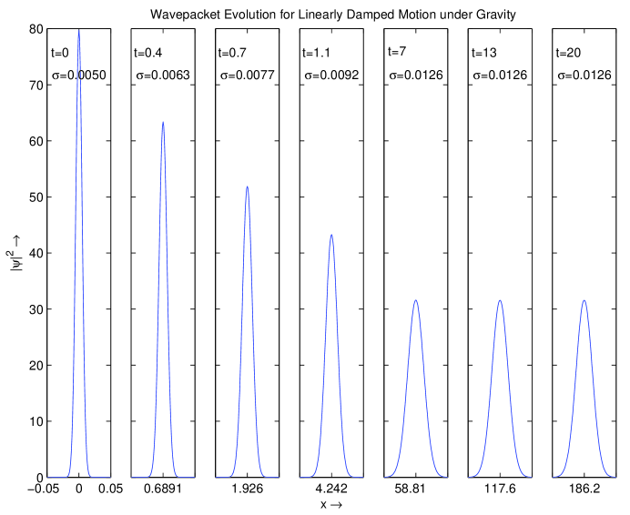
Figure 3: Evolution of wavepacket for motion under gravity with linear damping for the parameters $\Lambda=1.0$, $a=0.0$, and $g=9.8$.

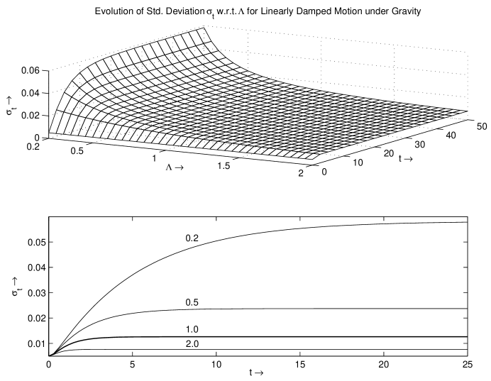
Figure 4: Variation of $\sigma_{t}$ with $t$ and $\Lambda$ for motion under gravity with linear damping [Eq. (20)]. The value of $\Lambda$ for each curve is shown just above the corresponding curve.

The wavepacket evolution is shown in Fig. 3, and the variation of $\sigma_{t}$ on the damping coefficient $\Lambda$ and the time $t$ is shown in Fig. 4. From Fig. 3 we see that the width of the wavepacket increases initially and then becomes almost constant as the exponential part of Eq. (20) decays. From Fig. 4 we see that the variance $\sigma_{t}$ exhibits the same generic behavior for all values of $\Lambda$. However, the time taken to reach a near-constant value of $\sigma$ is different for different $\Lambda$ values and represents the time needed to reach the terminal velocities in the corresponding cases. This behavior of the wavepacket seems to be characteristic of systems involving a terminal velocity though, as we show later there are interesting differences in the case for quadratic damping. The expectation value of $x$ is

$$\langle{x}\rangle=a+\frac{g}{\Lambda}t-\frac{g}{\Lambda^{2}}(1-e^{-\Lambda t}).$$ (22)

This result is the same as Eqs. (21) and (15) if the constants are evaluated using the initial conditions $x(0)=a$ and $\dot{x}(0)=0$.

IV Quadratic Damping

IV.1 Path Integral Kernel and wavepacket Evolution

We consider a particle moving in a uniform gravitational field with a damping force proportional to the square of its speed. Much work has been done on the quantization of this and similar systems with quadratic damping.razavy1 ; negro ; tartaglia ; negrotartag ; stuckens ; borges The equation of motion with this type of damping is $m\ddot{x}+\beta\dot{x}^{2}=mg$. Note that the equation is time-reversal invariant. The general solution is

$$x(t)=\frac{1}{\Lambda}\big{[}\ln[\cosh(\sqrt{g\Lambda}t+A)]\big{]}+B,$$ (23)

where $\Lambda=\beta/m$ and $A$ and $B$ are integration constants. The choice of a suitable Lagrangian for this case is interesting because there are nonequivalent Lagrangians which give rise to the same equation of motion. Consider for example the forms

$${\cal L} =\Big{(}\frac{1}{2}m\dot{x}^{2}+\frac{mg}{2\Lambda}\Big{)}e^{2\Lambda x},$$ (24)

$${\cal L} =-\sqrt{1-\frac{\Lambda}{g}\dot{x}^{2}}e^{-\Lambda x}.$$ (25)

To quantize the system we must judiciously choose the form that can be handled easily despite the fact that different Lagrangians can give rise to nonequivalent quantizations. The Lagrangian in Eq. (25) is not so easy to use because of the presence of the square root in the path integral method. Thus, we choose the Lagrangian in Eq. (24). Despite the presence of damping, the Lagrangians are not explicitly time-dependent unlike the damped harmonic oscillator or a particle in a gravitational field with linear damping. The Hamiltonian derived from Eq. (24) is a conserved quantity, but does not correspond to the energy of the system. A discussion on the conserved quantities in damped systems is given in Ref. denman, .

We note that although the Lagrangian (24) is not a quadratic Lagrangian, we can make it so by using the transformation: $X=\!\int e^{\Lambda x}dx=e^{\Lambda x}/\Lambda$.ambika This transformation converts it into a Lagrangian similar to that of an simple harmonic oscillator with imaginary frequency whose results are knownfeyn1 ; narlikar or can be deduced from those of Sec. III.1 by setting $\Lambda=0$.

We can write the action in terms of $X$ and $t$ as

$$S=\!\int_{t_{i}}^{t_{f}}\frac{m}{2}(\dot{X}^{2}+g\Lambda X^{2})dt.$$ (26)

If we compare Eq. (26) with the harmonic oscillator action given by:

$$S_{\rm HO}=\!\int_{t_{i}}^{t_{f}}\frac{m}{2}(\dot{x}^{2}-\omega^{2}x^{2})dt,$$ (27)

we obtain $\omega=i\sqrt{g\Lambda}=i\gamma$. We use the known results for the propagator of the harmonic oscillator and obtain the kernel in terms of $X$ and $\gamma$ as

$$K(X_{f},t_{f};X_{i},t_{i})=\sqrt{\frac{m\gamma}{2\pi i\hbar\sinh{\gamma T}}}\exp\Big{(}\frac{im\gamma}{2\hbar\sinh{\gamma T}}\big{[}(X_{i}^{2}+X_{f}^{2})\cosh{\gamma T}-2X_{i}X_{f}\big{]}\Big{)}.$$ (28)

If we transform back to $x$, we obtain the desired kernel:

$$K(x_{f},t_{f};x_{i},t_{i})=\sqrt{\frac{m\gamma}{2\pi i\hbar\sinh{\gamma T}}}\exp\Big{(}\frac{im\gamma}{2\hbar\Lambda^{2}\sinh{\gamma T}}\big{[}(e^{2\Lambda x_{i}}+e^{2\Lambda x_{f}})\cosh{\gamma T}-2e^{\Lambda(x_{i}+x_{f})}\big{]}\Big{)}.$$ (29)

The evolution of a Gaussian wavepacket in the $X$-coordinate will be similar to Eq. (9) and Eq. (11) (after setting $\Lambda=0$). Therefore, in terms of the $x$-coordinate we can write

$$\psi(x_{i},0)=\Big{(}\frac{1}{2\pi{\sigma_{0}}^{2}}\Big{)}^{1/4}\exp\Big{[}\frac{-\big{(}e^{\Lambda x_{i}}-e^{\Lambda a}\big{)}^{2}}{4\Lambda^{2}{\sigma_{0}}^{2}}\Big{]},$$ (30)

and

$$|\psi(x_{f},t)|^{2} =\frac{1}{\sqrt{2\pi{\sigma_{t}}^{2}}}\exp\Big{[}\frac{-\big{(}e^{\Lambda x_{f}}-e^{\Lambda a}\cosh{\gamma t}\big{)}^{2}}{2\Lambda^{2}{\sigma_{t}}^{2}}\Big{]},$$ (31)

$${\sigma_{t}}^{2} ={\sigma_{0}}^{2}\Big{[}\cosh^{2}{\gamma t}+\Big{(}\frac{\hbar\sinh\gamma t}{2m\gamma{\sigma_{0}}^{2}}\Big{)}^{2}\Big{]}.$$ (32)

If we set the exponent in Eq. (31) to zero, we see that the wavepacket is peaked at:

$$x_{f}=a+\frac{1}{\Lambda}\ln(\cosh\gamma t).$$ (33)

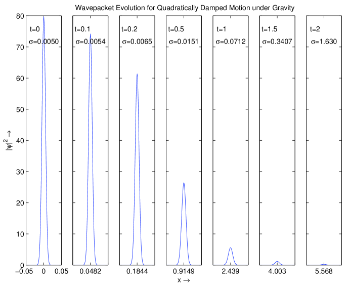
Figure 5: wavepacket evolution for motion under gravity with quadratic damping with $\Lambda=1.0$, $a=0.0$, and $g=9.8$.

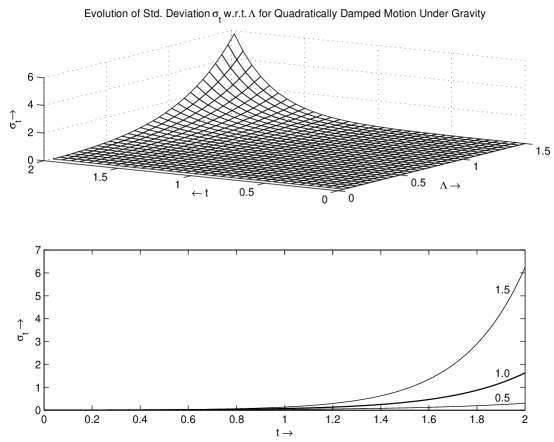
Figure 6: Variation of $\sigma_{t}$ with $t$ and $\Lambda$ for motion under gravity with quadratic damping, [Eq. (32)]. The value of $\Lambda$ for each curve is shown just above the corresponding curve.

The wavepacket evolution is shown in Fig. 5, and the variation of $\sigma_{t}$ with time $t$ and $\Lambda$ is shown in Fig. 6. From Figs. 5 and 6 we see that the width of the wavepacket increases indefinitely and rapidly. From Fig. 6 we see that the standard deviation $\sigma_{t}$ exhibits similar behavior for all values of the damping coefficient $\Lambda$. The only difference is the rate at which $\sigma_{t}$ grows, which can be derived from Eq. (32). Thus for motion under gravity, the linear and quadratic damping cases can be distinguished from each other by following the corresponding wavepacket evolution (see Fig.  4 for linear damping and Fig.  6 for quadratic damping).

As before, we would like to calculate the expectation value of $x$. We first calculate $\langle X\rangle$, which can be determined from Eq. (14) by setting $\Lambda=0$. Using the relation $X=\exp^{\Lambda x}/\Lambda$ we get

$$\langle{e^{\Lambda x}}\rangle=e^{\Lambda a}\cosh\gamma t.$$ (34)

If we expand the exponential on both sides and compare the coefficients of $\Lambda$, we obtain

$$\langle x\rangle=a+\frac{1}{\Lambda}\ln(\cosh\gamma t).$$ (35)

This result is the same as Eqs. (33) and (23).

IV.2 Connection with Field Theory

In the following we will show that the classical equation of motion for a particle subject to damping proportional to the square of the velocity can be obtained from a zero-dimensional version of the field theory of tachyon matter that emerges from string theorysayan1 . This example provides a link between a field theory and a damped mechanical system. Recall other such connections such as that between the simple harmonic oscillator and the massive Klein-Gordon field theory.

The action for the tachyontachyonclarify matter field in a $p+1$ dimensional spacetime is given assen1

$$S=-\!\int\!d^{p+1}\!x\,V(T)\sqrt{1+\eta^{ij}\partial_{i}T\partial_{j}T},$$ (36)

where $\eta_{ij}$ is the metric for a $(p+1)$-dimensional flat spacetime with components $\eta_{ij}\equiv{\rm diag}(-1,1,\ldots)$ for $i,\,j=0,\ldots,p$; $T(x)$ is the tachyon field, and $V(T)\sim e^{-\alpha T/2}$ denotes the corresponding field potential. The value of the parameter $\alpha$ depends on the particular type of string theory of interest.

We now consider the form of the action for a zero-space dimensional case, that is, $p=0$. We identify the tachyon field with the coordinate $x$ ($T\rightarrow x$) in the classical problem. Note that in classical mechanics the action has the form $S=\!\int\!Ldt$ and the zero-dimensional action has a similar form

$$S=-\!\int dt\,e^{-\alpha x}\sqrt{1-\dot{x}^{2}},$$ (37)

where the factor of 2 in the potential $V(x)$ has been absorbed in $\alpha$. The equation of motion that results from the action in Eq. (37) is

$$\ddot{x}+\alpha\dot{x}^{2}=\alpha.$$ (38)

We now scale $x\to bx$ and compare Eq. (38) with the equation of motion $\ddot{x}+\Lambda\dot{x}^{2}=g$. We obtain $\alpha b=\Lambda$ and $\alpha/b=g$, which can be solved to yield $\alpha=\sqrt{g\Lambda}$ and $b=\sqrt{\Lambda/g}$. We substitute these results into Eq. (37) and recover the Lagrangian in Eq. (25). Thus, we obtain a quadratically damped mechanical system out of a field theory.

IV.3 Damping as Geodesic Motion

Another way of looking at the problem of quadratically damped motion is to picture it as the motion of a particle along a geodesic in a fictitious two-dimensional space. Consider the following form of a two-dimensional distance function (line element)

$$ds^{2}=f(x)dx^{2}+h(x)dy^{2},$$ (39)

where $y$ denotes the fictitious dimension and $f(x)$ and $h(x)$ are unknown functions. Our aim is to show that for an appropriate choice of $f(x)$ and $h(x)$, the equation of motion for a quadratically damped system can be identified as a geodesic equation. For the metric $g_{\mu\nu}\equiv{\rm diag}[f(x),h(x)]$, we calculate the nonzero components of the Christoffel symbolsymbol :

$$\Gamma^{x}_{xx}=\frac{f^{\prime}}{2f},\qquad\Gamma^{x}_{yy}=-\frac{h^{\prime}}{2f},\quad\Gamma^{y}_{xy}=\frac{h^{\prime}}{2h}=\Gamma^{y}_{yx},$$ (40)

where the prime denotes the derivative of the function with respect to $x$. If we substitute these components into the well known geodesic equation given as

$$\frac{d^{2}x^{\alpha}}{d\lambda^{2}}+\Gamma^{\alpha}_{\mu\nu}\frac{dx^{\mu}}{d\lambda}\frac{dx^{\nu}}{d\lambda}=0,$$ (41)

(here $\lambda$ is any parameter on the geodesic, which in our case is the time $t$), we obtain the equation of motion along the two directions:

$$\ddot{x}+\frac{f^{\prime}}{2f}\dot{x}^{2}-\frac{h^{\prime}}{2f}\dot{y}^{2} =0,$$ (42)

$$\ddot{y}+\frac{h^{\prime}}{h}\dot{x}\dot{y} =0.$$ (43)

If we integrate Eq. (43) once, we have

$$\dot{y}=\frac{C}{h},$$ (44)

where $C$ is an integration constant. We next substitute $\dot{y}$ in Eq. (42) and obtain

$$\ddot{x}+\frac{f^{\prime}}{2f}\dot{x}^{2}-\frac{C^{2}h^{\prime}}{2fh^{2}}=0,$$ (45)

which is the same equation as the quadratically damped equation of motion along the $x$ direction provided that $f^{\prime}/2f=\Lambda$ and $C^{2}h^{\prime}/2fh^{2}=g$. These equations can be solved to reveal the form of the two functions:

$$f(x) =e^{2\Lambda x}$$ (46)

$$h(x) =-\frac{C^{2}\Lambda}{g}e^{-2\Lambda x}.$$ (47)

It is now straightforward to calculate the components of the Riemann tensor, ${R^{\alpha}}_{\beta\mu\nu}$,foot Ricci tensor, $R_{\mu\nu}={R^{\alpha}}_{\mu\alpha\nu}$, and the Ricci scalar, $R=g^{\mu\nu}R_{\mu\nu}$:gravdesc

$$R_{xx}=-2\Lambda^{2},\quad R_{yy}=\frac{2C^{2}\Lambda^{3}}{g}e^{-2\Lambda x},\quad R=-4\Lambda^{2}e^{-2\Lambda x}.$$ (48)

The presence of $\Lambda$ in the curvature scalar $R$ implies that the damping can be viewed as a curvature effect in this fictitious two-dimensional space. What distinguishes this case from the motion with linear damping discussed in section IIIB is that we cannot cast the equation of motion of the linear damping case in the form of a geodesic equation due to the absence of a $\dot{x}^{2}$ term. In this sense, quadratic damping is unique. Thus the above connection provides us with additional geometric insight into the nature of quadratically damped motion.

V Concluding Remarks

We have shown how to construct kernels for several damped mechanical systems and studied the evolution of a Gaussian wavepacket in each case. We demonstrated that for the linearly damped harmonic oscillator and a particle in a uniform gravitational field with linear and quadratic damping, we can see characteristic features of the damping from snapshots of wavepacket evolution. To motivate our consideration of quadratic damping, we related the corresponding equation of motion to a field theory and to geodesic motion in a fictitious two-dimensional space.

Is a quadratically damped system damped? The Lagrangian is time independent and the system is Hamiltonian and conservative in the usual sense. The evolution of the wavepacket shows spreading, much like that of a free particle and unlike the linear damping system. We also note a similarity with the linearly damped system because in both cases, the particle attains a terminal speed. These issues suggest that it would be better to view the quadratically damped system as special and unlike the linearly damped case.

Tables

Case	$x(t)$	$A$	$B$
OD	$e^{-\Lambda t/2}[A\cosh{\gamma t}+B\sinh{\gamma t}]$	$\frac{[x_{i}e^{\Lambda t_{i}/2}\sinh\gamma t_{f}-x_{f}e^{\Lambda t_{f}/2}\sinh\gamma t_{i}]}{\sinh{\gamma T}}$	$\frac{1}{\sinh\gamma T}[x_{f}e^{\Lambda t_{f}/2}\cosh\gamma t_{i}-x_{i}e^{\Lambda t_{i}/2}\cosh\gamma t_{f}]$
CD	$e^{-\Lambda t/2}[A+Bt]$	$\frac{1}{T}[x_{i}t_{f}e^{\Lambda t_{i}/2}-x_{f}t_{i}e^{\Lambda t_{f}/2}]$	$\frac{1}{T}[x_{f}e^{\Lambda t_{f}/2}-x_{i}e^{\Lambda t_{i}/2}]$
UD	$e^{-\Lambda t/2}[A\cos{\omega t}+B\sin{\omega t}]$	$\frac{[x_{i}e^{\Lambda t_{i}/2}\sin\omega t_{f}-x_{f}e^{\Lambda t_{f}/2}\sin\omega t_{i}]}{\sin{\omega T}}$	$\frac{1}{\sin\omega T}[x_{f}e^{\Lambda t_{f}/2}\cos\omega t_{i}-x_{i}e^{\Lambda t_{i}/2}\cos\omega t_{f}]$

Table 1: The general solutions of the equations of motion of a damped harmonic oscillator in different cases. We show the expressions for $x(t)$, $A$, and $B$ for the different cases. (See the discussion in section IIIA.)

Case	S (Action)	K (Kernel)
CD	$\frac{m}{2T}[x_{i}^{2}e^{\Lambda t_{i}}+x_{f}^{2}e^{\Lambda t_{f}}-2x_{i}x_{f}e^{\Lambda(t_{i}+t_{f})/2}]+\frac{m\Lambda}{4}(x_{i}^{2}e^{\Lambda t_{i}}-x_{f}^{2}e^{\Lambda t_{f}})$	$\sqrt{\frac{me^{\Lambda(t_{i}+t_{f})/2}}{2\pi i\hbar T}}e^{\frac{i}{\hbar}S}$
OD	$\frac{m\gamma}{2\sinh{\gamma T}}[(x_{i}^{2}e^{\Lambda t_{i}}+x_{f}^{2}e^{\Lambda t_{f}})\cosh\gamma T-2x_{i}x_{f}e^{\Lambda(t_{i}+t_{f})/2}]+$	$\sqrt{\frac{m\gamma e^{\Lambda(t_{i}+t_{f})/2}}{2\pi i\hbar\sinh{\gamma T}}}e^{\frac{i}{\hbar}S}$
	$\frac{m\Lambda}{4}(x_{i}^{2}e^{\Lambda t_{i}}-x_{f}^{2}e^{\Lambda t_{f}})$

Table 2: Action $(S)$ and Kernel $(K)$ for the critically and over–damped harmonic oscillator.

Case	$|\psi(x_{f},t)|^{2}$	${\sigma_{t}}^{2}$
CD	$\frac{1}{\sqrt{2\pi{\sigma_{t}}^{2}}}\exp[\frac{-\big{[}x_{f}-ae^{-\Lambda t/2}\big{(}1+\frac{\Lambda t}{2}\big{)}\big{]}^{2}}{2{\sigma_{t}}^{2}}\big{]}$	${\sigma_{0}}^{2}e^{-\Lambda t}\big{[}\big{(}1+\frac{\Lambda t}{2}\big{)}^{2}+\big{(}\frac{\hbar t}{2m{\sigma_{0}}^{2}}\big{)}^{2}\big{]}$
OD	$\frac{1}{\sqrt{2\pi{\sigma_{t}}^{2}}}\exp\big{[}\frac{-\big{[}x_{f}-ae^{-\Lambda t/2}(\cosh\gamma t+\frac{\Lambda}{2\gamma}\sinh\gamma t)\big{]}^{2}}{2{\sigma_{t}}^{2}}\big{]}$	${\sigma_{0}}^{2}e^{-\Lambda t}\big{[}\big{(}\cosh\gamma t+\frac{\Lambda}{2\omega}\sinh\gamma t\big{)}^{2}+\big{(}\frac{\hbar\sinh\gamma t}{2m\gamma{\sigma_{0}}^{2}}\big{)}^{2}\big{]}$

Table 3: Probability amplitude $|\psi(x_{f},t)|^{2}$ and measure of dispersion $\sigma_{t}^{2}$ for the critically (CD) and over-damped (OD) harmonic oscillator.

Figure Captions