Decoherence induced by interacting quantum spin baths

Abstract

We study decoherence induced on a two-level system coupled to a one-dimensional quantum spin chain. We consider the cases where the dynamics of the chain is determined by the Ising, $XY$, or Heisenberg exchange Hamiltonian. This model of quantum baths can be of fundamental importance for the understanding of decoherence in open quantum systems, since it can be experimentally engineered by using atoms in optical lattices. As an example, here we show how to implement a pure dephasing model for a qubit system coupled to an interacting spin bath. We provide results that go beyond the case of a central spin coupled uniformly to all the spins of the bath, in particular showing what happens when the bath enters different phases, or becomes critical; we also study the dependence of the coherence loss on the number of bath spins to which the system is coupled and we describe a coupling-independent regime in which decoherence exhibits universal features, irrespective of the system-environment coupling strength. Finally, we establish a relation between decoherence and entanglement inside the bath. For the Ising and the $XY$ models we are able to give an exact expression for the decay of coherences, while for the Heisenberg bath we resort to the numerical time-dependent Density Matrix Renormalization Group.

I Introduction

Decoherence refers to the process through which superpositions of quantum states are irreversibly transformed into statistical mixtures. It is due to the unavoidable coupling of a quantum system with its surrounding environment which, as a consequence, leads to entanglement between the system and the bath. This loss of coherence may considerably reduce the efficiency of quantum information protocols nielsen and it is crucial in describing the emergence of classicality in quantum systems zurek .

Although desirable, it is not always possible to fully characterize the bath. Therefore it is necessary to resort to ingenious, though realistic, modelizations. Paradigmatic models represent the environment as a many-body system, such as a set of bosonic harmonic oscillators caldeira ; weiss or of spin-1/2 particles prokofiev . In some cases it is also possible to recover the effects of a many-body environment via the coupling to a single-particle bath, provided its dynamics is chaotic benenti . In order to grasp all the subtleties of the entanglement between the system and its environment, it would be of great importance to study engineered baths (and system-bath interactions) that can be realized experimentally. In this paper we discuss a class of interacting spin baths which satisfy these requirements: a two-level system coupled to a one-dimensional array of spin-1/2 particles, whose free evolution is driven by a Hamiltonian which embraces Ising, $XY$ and Heisenberg universality classes. In several non-trivial cases we can solve the problem exactly. Moreover we show that it is possible to realize these system+bath Hamiltonians with cold bosons in optical lattices. We thus extend the approach of Jané et al. jane03 showing that optical lattices can be useful as open quantum system simulators.

Our analysis can be framed in the context of the recently growing interest in the study of decoherence due to spin baths, see zurek2 ; cucchietti ; tessieri ; dawson ; paganelli ; quan ; cucchietti2 ; ou06 ; khveshchenko ; dobrovitski ; lages ; camalet ; zurek3 . Starting from the seminal paper of Zurek zurek2 , several papers analyzed the decoherence due to a collection of independent spins. Cucchietti, Paz and Zurek cucchietti derived several properties of the Loschmidt echo starting from fairly general assumptions for the distribution of the splittings of the bath spins. The effect of an infinite-range interaction among the spins was introduced in Ref. tessieri ; the same model was further exploited in Dawson et al. dawson to relate decoherence to the entanglement present in the bath. Properties of decoherence in presence of symmetry breaking, and the effect of critical behavior of the bath were discussed in paganelli ; quan . Most of the works done so far are based on the so called central spin model, where the two-level system is coupled isotropically to all the spins of the bath. This assumption tremendously simplifies the derivation, but at the same time it may introduce some fictitious symmetries which are absent in realistic systems. Moreover it can be very hard to simulate it with engineered baths. A crucial feature of our work is the assumption that the two-level system interacts with only few spins of the bath. As we will show, this introduces qualitative differences as compared to the central spin model, moreover it is amenable to an experimental implementation with optical lattices.

The paper is organized as follows. In the next Section we introduce the system+bath model Hamiltonians that will be studied throughout this paper and we define the central quantity that will be used in order to characterize the decoherence of the system, i.e. the Loschmidt echo. We then show in Section III how optical lattices can be used to simulate the class of Hamiltonians introduced in Section II. The rest of the paper is devoted to the derivation and to the analysis of our results, both for a single system-bath link (Section IV), and for multiple links (Section V). When the two-level system is coupled to an $XY$- or $XX$-model, it is possible to derive an exact result for the Loschmidt echo. This is explained in Section IV.1, where we also discuss in detail its short- and long-time behavior and relate it to the critical properties of the chain. Further insight is obtained by perturbative calculations which agree very well, in the appropriate limits, with the exact results. In Section IV.2 we present our results for the Heisenberg bath. In this case an analytic approach is not possible. Here we solve the problem by means of the time-dependent Density Matrix Renormalization Group (t-DMRG – see Appendix A). In Section IV.3 we analyze the possible relation between decoherence and entanglement properties of the environment: we relate the short-time decay of coherences to the two-site nearest-neighbor concurrence inside the bath. In Section V we extend our results to the case in which the system is coupled to an arbitrary number of bath spins; a regime in which the decoherence is substantially independent of the coupling strength between the system and the environment is discussed in Section V.1. Finally, in Section VI we draw our conclusions. In the Appendices we give some technical details on the numerical DMRG approach (Appendix A), we provide explicit expressions for the Fermion correlation functions needed for the evaluation of the Loschmidt echo in the $XY$-model (Appendix B) and we briefly discuss the central spin model (Appendix C) to make our paper self-contained. A brief account of some of the results discussed in this paper is presented in rossini06 .

II The model

The model we consider consists of a two-level quantum object (qubit) $S$ coupled to an interacting spin bath $E$ composed by $N$ spin-$1/2$ particles (see Fig.1a): the idea is to study how the internal dynamics of $E$ affects the decoherent evolution of $S$.

In our scheme the global system $S+E$ is fully characterized by a standard Hamiltonian of the form

$$\mathcal{H}=\mathcal{H}_{S}+\mathcal{H}_{E}+\mathcal{H}_{\mathrm{int}}\,,$$ (1)

with $\mathcal{H}_{S,E}$ being the free-Hamiltonians of $S$ and $E$, and $\mathcal{H}_{\mathrm{int}}$ being the coupling term. Without loss of generality we will assume the free Hamiltonian of the qubit to be of the form

$$\mathcal{H}_{S}=\frac{\omega_{e}}{2}\left(\mathbbm{1}-\tau_{z}\right)=\omega_{e}\left|e\right\rangle\left\langle e\right|\,,$$ (2)

with $\tau_{\alpha}$ being the Pauli matrices of $S$ ($\alpha=x,y,z$), and $\left|e\right\rangle$ its excited state (the ground state being represented by the vector $\left|g\right\rangle$). On the other hand, the environment will be modeled by a one-dimensional quantum spin-1/2 chain described by the Hamiltonian

$$\mathcal{H}_{E} = -\frac{J}{2}\sum_{j}\left[\left(1+\gamma\right)\sigma^{x}_{j}\sigma^{x}_{j+1}+\left(1-\gamma\right)\sigma^{y}_{j}\sigma^{y}_{j+1}\right.$$ (3)

$$+\left.\Delta\sigma^{z}_{j}\sigma^{z}_{j+1}+2\lambda\sigma^{z}_{j}\right]\,,$$

where $\sigma^{\alpha}_{i}$ ($\alpha=x,y,z$) are the Pauli matrices of the $i$-th spin. The sum over $j$ goes from 1 to $N-1$ for open boundary conditions, or from 1 to $N$ for periodic boundary conditions (where we assume that $\sigma^{\alpha}_{N+1}\equiv\sigma^{\alpha}_{1}$). The constants $J$, $\Delta$, $\gamma$ and $\lambda$ respectively characterize the interaction strength between neighboring spins, the anisotropy parameter along $z$ and in the $xy$ plane, and an external transverse magnetic field. The Hamiltonian (3) has a very rich structure sachdev99 . For the sake of simplicity, we shall consider the following paradigmatic cases:

• the $XY$-model in a transverse field – see Sec. IV.1. Here one has $\Delta=0$ and $\lambda$, $\gamma$ generic. For $0<\gamma\leq 1$, Eq. (3) belongs to the Ising universality class, and it has a critical point at $|\lambda_{c}|=1$; for $\gamma=0$ it reduces to the $XX$ universality class, which is critical for $|\lambda|\leq 1$.

• the $XXZ$ anisotropic Heisenberg model – see Sec. IV.2. Here one has $\lambda,\gamma=0$ and $\Delta$ generic. In this case the Hamiltonian (3) is critical for $-1\leq\Delta\leq 1$ while it has ferromagnetic or anti-ferromagnetic order for $\Delta>1$ or $\Delta<-1$ respectively.

Finally, the qubit $S$ is coupled to the spin bath through a dephasing interaction of the form

$$\mathcal{H}_{\mathrm{int}}=-\epsilon\sum_{j=j_{1}}^{j_{m}}\left|e\right\rangle\left\langle e\right|\sigma_{j}^{z}\,,$$ (4)

where $\epsilon$ is the coupling constant, and the link number $m$ counts the number of environmental spins (labeled by $j_{1}\ldots j_{m}$) to which $S$ is coupled — Fig.1a refers to the case where $S$ is interacting with the first spin of an open-boundary chain, i.e. $m=1$, $j_{1}=1$.

By varying the parameters $m,\Delta,\gamma,\lambda$ and $\epsilon$, the above Hamiltonians allow us to analyze several non-trivial $S+E$ scenarios. Moreover we will see in Sec. III that it is possible to use optical lattices manipulation techniques duan03 ; jane03 to experimentally simulate the resulting dynamical evolution.

II.1 Decoherence: the Loschmidt echo

With the choice of the coupling (4) the populations of the ground and excited states of the qubit do not evolve in time, since $[\tau^{z},\mathcal{H}]=0$. Consequently, no dissipation takes place in the model and the qubit evolution is purely decoherent: the system $S$ looses its coherence without exchanging energy with the bath unruh ; palma . To study this effect of pure phase decoherence, we suppose that at the beginning the qubit is completely disentangled from the environment — namely, at time $t=0$ the global system wave-function is given by

$$\left|\Psi(0)\right\rangle=|\phi(0)\rangle_{S}\otimes|\varphi(0)\rangle_{E}\,,$$ (5)

where $|\phi(0)\rangle_{S}=c_{g}\left|g\right\rangle+c_{e}\left|e\right\rangle$ is a generic superposition of the ground and the excited state of $S$ and $|\varphi(0)\rangle_{E}\equiv\left|G\right\rangle_{E}$ is the ground state of the environment Hamiltonian $\mathcal{H}_{E}$. The global evolution of the composite system under the Hamiltonian Eq. (1) will then split into two terms: one where $E$ evolves with the unperturbed Hamiltonian $\mathcal{H}_{g}\equiv\mathcal{H}_{E}$ and the other where $E$ evolves with the perturbed Hamiltonian

$$\mathcal{H}_{e}\equiv\mathcal{H}_{E}+\langle e|\mathcal{H}_{\mathrm{int}}|e\rangle\;.$$ (6)

As a result, one has

$$\left|\Psi(0)\right\rangle\to\left|\Psi(t)\right\rangle = c_{g}\left|g\right\rangle\otimes\left|\varphi_{g}(t)\right\rangle_{E}$$

$$+ c_{e}e^{-i\omega_{e}t}\left|e\right\rangle\otimes\left|\varphi_{e}(t)\right\rangle_{E}$$

where the two branches of the environment are $\left|\varphi_{g}(t)\right\rangle_{E}=e^{-i\mathcal{H}_{g}t}\left|\varphi(0)\right\rangle_{E}$ and $\left|\varphi_{e}(t)\right\rangle_{E}=e^{-i\mathcal{H}_{e}t}\left|\varphi(0)\right\rangle_{E}$. Therefore the evolution of the reduced density matrix $\rho\equiv\mathrm{Tr}_{E}\left|\Psi\right\rangle\left\langle\Psi\right|$ of the two-level system corresponds to a pure dephasing process. In the basis of the eigenstates $\{\left|g\right\rangle$, $\left|e\right\rangle\}$, the diagonal terms $\rho_{gg}$ and $\rho_{ee}$ do not evolve in time. Instead the off-diagonal terms will decay according to

$$\rho_{eg}(t)=\rho_{eg}(0)\,e^{-i\omega_{e}t}D(t)\;,$$

where

$$D(t)\equiv\langle\varphi_{g}(t)|\varphi_{e}(t)\rangle=\langle\varphi(0)|e^{i\mathcal{H}_{g}t}e^{-i\mathcal{H}_{e}t}|\varphi(0)\rangle\,$$ (8)

is the decoherence factor. The decoherence of $S$ can then be characterized by the so-called “Loschmidt echo”, i.e. by the real quantity

$$\mathcal{L}(t)\equiv|D(t)|^{2}=|\langle G|e^{-i(\mathcal{H}_{E}+\langle e|\mathcal{H}_{\mathrm{int}}|e\rangle)t}|G\rangle|^{2}\,,$$ (9)

where in the equality term we used the fact that $|\varphi(0)\rangle=|G\rangle$ is the ground state of $\mathcal{H}_{E}$. On one hand, values of $\mathcal{L}(t)$ close to $1$ indicate a weak interaction between the environment and the qubit (the case $\mathcal{L}(t)=1$ corresponds to total absence of interaction). On the other hand, values of $\mathcal{L}(t)$ close to $0$ correspond instead to a strong suppression of the qubit coherence due to the interaction with $E$ (for $\mathcal{L}(t)=0$ the qubit is maximally entangled with the environment, and its density matrix $\rho$ becomes diagonal). In the following we will analyze the time evolution of the Loschmidt echo to study how the internal dynamics of the environment $E$ affects the decoherence of the system $S$. We will start with the case when $S$ is coupled to a single spin of the chain $E$ (i.e. $m=1$, see Sec. IV). The case with multiple links will be instead discussed in Sec. V.

For the sake of completeness, we finally notice that, since the function (9) measures the overlap between the time-evolved states of the same initial configuration under two slightly different Hamiltonians, one can use it as an indicator of the stability of motion. This kind of analysis has been performed in Ref. zanardi06 , where the fidelity between the ground states of quadratic Fermi Hamiltonians has been analyzed in connection with quantum phase transitions.

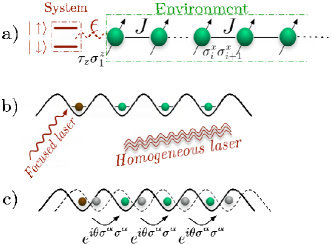
Figure 1: a) A sketch of the system-plus-bath model we consider in this work. The two-level system (at position zero) is coupled to the $\sigma^{z}$ component of the first spin of the chain that acts as a spin bath. Atoms in an optical lattice can simulate this controlled decoherence by means of series of lasers b) and lattice displacements c), which allow to realize both the interaction of the bath with an external magnetic field and the anisotropic exchange coupling present in Eq. (3).

III Simulation of open quantum systems by optical lattices

Before analyzing in detail the temporal evolution of the Loschmidt echo (9), in this Section we present a method which would allow one to experimentally simulate the dynamics induced by the Hamiltonian of Eq. (1) in a realistic setup.

The $S+E$ system introduced in Sec. II can be seen as an “inhomogeneous” spin network with $N+1$ sites, where one of the spins (say, the first) plays the role of the system of interest $S$ while the remaining $N$ play the role of the environment $E$. This immediately suggests the possibility of simulating the dynamical evolution of such a system on optical lattices by employing the techniques recently developed in Refs. duan03 ; jane03 . An important aspect of our scheme however is the fact that we assume the coupling between the system $S$ and $E$ to be independent from the couplings among the $N$ spins which compose the environment. Analogously the free Hamiltonian of $S$ is assumed to be different from the on-site terms of the free-Hamiltonian of $E$. On one hand this allows us to study different environment Hamiltonians without affecting the coupling between $E$ and $S$. On the other hand, this also allow us to analyze different $S+E$ coupling regimes (e.g. strong, weak) without changing the internal dynamics of the bath.

In order to include these crucial ingredients we found more convenient to follow the scheme developed by Jané et al. in Ref. jane03 (the optical lattice manipulation schemes developed by Duan et al. in Ref. duan03 seem to be less adequate to our purposes). The key advantage is that we can realize the system-plus-bath setup by using a single one-dimensional lattice in which the quantum system is placed on a given lattice site (for example the first one, as in Fig. 1b). The different Hamiltonians for the system and for the bath are realized by specific pulse sequences which simulate the dynamics of the model. The same holds for the coupling Hamiltonian of the two-level system with the bath, which is different from the couplings within the bath. In Fig. 1 the leftmost atom simulates the two-level system, the coupling to the second site is the interaction between the quantum system and the environment, the rest of the chain is the interacting spin environment.

Jané et al. jane03 showed that atoms loaded in an optical lattice can simulate the evolution of a generic spin Hamiltonian in a stroboscopic way when subjected to appropriate laser pulses, Fig. 1b, and controlled displacements, Fig. 1c, which allow to implement the single-site and two-site contributions to the Hamiltonian. The key point is that in our case the sequences of gates need to allow for discriminating between the system and the bath. The types of baths that one can simulate by these means embrace Ising, $XY$ and Heisenberg exchange Hamiltonian. Therefore, by varying the parameters of the optical lattice, it is possible to test the impact of the different phases (critical, ferromagnetic, anti-ferromagnetic, etc$\dots$) of the environment on the decoherence of the two-level system.

Following the idea of a Universal Quantum Simulator described in jane03 , the time evolution operator associated with ${\cal H}$ over a time $t$ can be simulated by decomposing it into a product of operators acting on very short times $\tau\ll t$:

$$e^{-i{\cal H}t} = \lim_{n\to\infty}\Bigg{[}U^{z}_{0}(\omega_{e}\tau)\,U^{zz}_{0,1}(\epsilon\tau)\,\prod_{j=1}^{N}U^{z}_{j}\big{(}\textstyle\frac{J\lambda\tau}{2}\big{)}$$

$$\times U^{xx}_{j,j+1}\big{(}\textstyle\frac{J(1+\gamma)\tau}{2}\big{)}\,U^{yy}_{j,j+1}\big{(}\textstyle\frac{J(1-\gamma)\tau}{2}\big{)}\,U^{zz}_{j,j+1}\big{(}\textstyle\frac{J\Delta\tau}{2}\big{)}\!\Bigg{]}^{n}$$

where $\tau=t/n$, $U^{z}_{j}(\theta)\equiv e^{i\theta\sigma_{j}^{z}}$, $U^{\alpha\beta}_{j,k}(\theta)\equiv e^{i\theta\sigma_{j}^{\alpha}\sigma_{k}^{\beta}}$, and the index $0$ labels the two-level system $S$. For $\alpha\in\{x,y\}$ one can write $U^{\alpha\alpha}_{j,k}=V^{\alpha}_{j}V^{\alpha}_{k}U^{zz}_{j,k}V^{\alpha\dagger}_{k}V^{\alpha\dagger}_{j}$, where $V^{\alpha}_{j}=(\openone-i\sigma^{\alpha}_{j})/\sqrt{2}$ are fast homogeneous local unitary operations. These can be realized with single atoms trapped in an optical lattice jane03 , each having two relevant electronic levels ($|0\rangle_{j}\,,\,|1\rangle_{j}$) interacting with a resonant laser according to:

$${\cal H}^{L}_{j}=\Omega\left(e^{i\phi}|1\rangle_{j}\langle 0|+e^{-i\phi}|0\rangle_{j}\langle 1|\,\right)\,.$$ (11)

The evolution under the Hamiltonian Eq. (11), $U^{L}_{j}(t,\phi)\equiv e^{-i{\cal H}^{L}_{j}t}$, yields the single-qubit operations $V^{x}_{j}=U^{L}_{j}(\frac{\pi}{4\Omega},0)$, $V^{y}_{j}=U^{L}_{j}(\frac{\pi}{2\Omega},0)\,U^{L}_{j}(\frac{3\pi}{4\Omega},\frac{\pi}{2})$ and $U^{z}_{j}(\theta)=U^{L}_{j}(\frac{\pi}{2\Omega},\pi+\theta)\,U^{L}_{j}(\frac{\pi}{2\Omega},0)$, whence $U^{z}_{j}(-\frac{\pi}{2})=i\sigma^{z}_{j}$, while $U^{L}_{j}(\frac{\pi}{2\Omega})=i\sigma^{x}_{j}$. These operation can be made very fast by simply increasing the laser intensity and thereby the Rabi frequency. They can be performed either simultaneously on all qubits, by shining the laser homogeneously onto all atoms, or selectively on some of them, by focusing it appropriately (see Fig. 1b). For our purposes the individual addressing is needed only for the atom in position $0$, which represents the quantum system; this is anyway the minimal physical requirement for being able to monitor its state during the evolution.

Two-qubit operations can be performed by displacing the lattice in a state-selective way Jaksch , so that state $|0\rangle_{j}|1\rangle_{j+1}$ acquires a phase factor $e^{-i\varphi}$, as experimentally realized in Bloch . The resulting gate $G_{j,j+1}(\varphi)$ can be composed with $\sigma^{x}$ rotations to yield $U^{zz}_{j,j+1}(\theta)=e^{i\theta}[G_{j,j+1}(2\theta)\,\sigma^{x}_{j}\sigma^{x}_{j+1}]^{2}$. This will affect all atoms from $0$ to $N$. Since we want a different coupling for the $\{01\}$ pair than for all others, we need to erase the effect of the interaction for that specific pair using only local operations on atom $0$, as in the sequences $[\sigma^{z}_{0}\,U^{xx}_{01}(\theta)]^{2}=[\sigma^{z}_{0}\,U^{yy}_{01}(\theta)]^{2}=[\sigma^{x}_{0}\,U^{zz}_{01}(\theta)]^{2}=\openone.$ Defining $U^{\alpha\alpha}_{\otimes}(\theta)\equiv\prod_{j=1}^{N}U^{\alpha\alpha}_{j,j+1}(\theta)$, we can generate each simulation step in Eq. (III) as

$${\cal U}_{n} \equiv \big{[}\sigma^{x}_{0}\,U^{zz}_{\otimes}\big{(}(\epsilon-\textstyle\frac{J\Delta}{2})\frac{\tau}{2}\big{)}\big{]}^{2}\,\big{[}\sigma^{z}_{0}U^{xx}_{\otimes}\big{(}-\textstyle\frac{J(\gamma+1)\tau}{4}\big{)}\big{]}^{2}$$

$$\big{[}\sigma^{z}_{0}\,U^{yy}_{\otimes}\big{(}\textstyle\frac{J(\gamma-1)\tau}{4}\big{)}\big{]}^{2}\,U^{zz}_{\otimes}(-\epsilon\tau)\,U^{z}_{0}(\omega_{e}\tau)\,U^{z}_{\otimes}\big{(}\textstyle\frac{J\lambda\tau}{2}\big{)}$$

involving only global lattice displacements, global laser-induced rotations and local addressing of atom $0$.

We note that an alternative scheme exists duan03 , based on tunnel coupling between neighboring atoms rather than on lattice displacements, which can attain the simulation described here for the special case $\gamma=0$ and would require some additional stroboscopic steps in order to reproduce the general case.

Apart from 1D spin baths, this approach can be extended to other types of environment. For example, it would be quite interesting to consider, as an engineered bath, a 3D optical lattice. Besides being feasible from an experimental point of view, this could be useful in studying for instance the situation found in solid-state NMR cory . It would be also intriguing to study the Bose-Hubbard model as a bath, which would make the experimental realization even simpler cucchietti06 . Here we just focus on one-dimensional baths since, in several cases, they are amenable to an exact solution.

IV Results: the single-link scenario

In this Section we analyze the time evolution of the Loschmidt echo from Eq. (9) for several distinct scenarios where the qubit $S$ is coupled to just one spin of the chain, i.e. $m=1$ in Eq. (4). In this case, in the thermodynamic limit the interaction $\mathcal{H}_{\mathrm{int}}$ between the system $S$ and the environment $E$ does not affect the description of the bath Hamiltonian $\mathcal{H}_{E}$, since it is local; therefore it can be considered in all senses as a small perturbation of the environment. The bath is effectively treated as a reservoir, which is in contact with the system through just one point. In the following we study the cases in which the bath is described by a one dimensional spin-1/2 Ising, an $XY$ (Subsec. IV.1) and a Heisenberg (Subsec. IV.2) chain.

IV.1 $XY$-bath

Here we focus on the case of a spin bath $E$ characterized by a free Hamiltonian (3) of the $XY$ form, i.e., with null anisotropy parameter along $z$ ($\Delta=0$). In this case the environment is a one-dimensional spin-1/2 $XY$-model, which is analytically solvable lieb61 . Below we show that also the Loschmidt echo can be evaluated exactly rossini06 , both for open and for periodic boundary conditions.

In the case $m<N$ in which the system $S$ is coupled to just some of the spins of the bath $E$, the perturbed Hamiltonian $\mathcal{H}_{e}$ of Eq. (6) is the Hamiltonian of an $XY$ chain in a non-uniform magnetic field. In this circumstance one cannot employ the approach of Ref. quan , and in general the dynamical evolution of the system has to be solved numerically. The derivation we present here instead is analytical and it applies for all values of $m=1,\cdots,N$. In the following we will present it for the case of a generic $m$ but, in the remaining of the Section, we will explicitly discuss its results only for the single-link case (i.e. $m=1$).

The first step of the analytical derivation is a Jordan-Wigner transformation (JWT), in order to map both Hamiltonians $\mathcal{H}_{g}$ and $\mathcal{H}_{e}$ onto a free-Fermion model, described by the quadratic form lieb61

$$\mathcal{H}=\sum_{i,j}\left[c_{i}^{\dagger}A_{i,j}c_{j}+\frac{1}{2}(c_{i}^{\dagger}B_{i,j}c_{j}^{\dagger}+\mathrm{h.c.})\right]+\frac{1}{2}\sum_{i}A_{i,i}\,,$$ (13)

where $c_{i},c_{i}^{\dagger}$ are the annihilation and creation operators for the spinless Jordan-Wigner fermions, defined by

$$c_{k}=\exp\bigg{(}i\pi\sum_{j=1}^{k-1}\sigma_{j}^{+}\sigma_{j}^{-}\bigg{)}\,\sigma_{k}^{-}\;.$$

The two matrices A, B are given by

$$\left[{\bf A}\right]_{j,k} = -J\big{(}\delta_{k,j+1}+\delta_{j,k+1}\big{)}-2(\lambda+\epsilon_{j})\delta_{j,k},$$ (14)

$$\left[{\bf B}\right]_{j,k} = -\gamma J\big{(}\delta_{k,j+1}-\delta_{j,k+1}\big{)}\,,$$ (15)

where $\epsilon_{j}=0$ for $\mathcal{H}_{g}$, while

$$\epsilon_{j}=\left\{\begin{array}[]{ll}\epsilon&\>\textrm{if S is coupled to the }j\textrm{-th spin}\\ 0&\>\textrm{elsewhere }\end{array}\right.$$ (16)

for $\mathcal{H}_{e}$. A generic quadratic form, like Eq. (13) (where A is a Hermitian matrix, due to the Hermiticity of $\mathcal{H}$, and B is antisymmetric, due to the anti-commutation rules among the $c_{i}$), can be diagonalized in terms of the normal-mode spinless Fermi operators $\{\eta_{k},\eta_{k}^{\dagger}\}$:

$$\mathcal{H}=\sum_{k}E_{k}\left(\eta_{k}^{\dagger}\eta_{k}-\frac{1}{2}\right),$$ (17)

where $\eta_{k}=\sum_{i}(g_{k,i}c_{i}+h_{k,i}c_{i}^{\dagger})$, or in matrix form:

$$\vec{\eta}={\bf g}\cdot\vec{c}+{\bf h}\cdot\vec{c}\,\,{}^{\dagger}\,.$$ (18)

If we rewrite the two change-of-basis matrices ${\bf g}$ and ${\bf h}$ as $g_{k,i}\equiv\frac{1}{2}(\phi_{k,i}+\psi_{k,i})$ and $h_{k,i}\equiv\frac{1}{2}(\phi_{k,i}-\psi_{k,i})$, we eventually arrive at the following coupled linear equations, whose solution permits to find the eigenbasis of the non-uniform Hamiltonian in Eq. (13):

$$\left\{\begin{array}[]{lcl}\vec{\phi}_{k}({\bf A}-{\bf B})&=&E_{k}\vec{\psi}_{k},\\ \vec{\psi}_{k}({\bf A}+{\bf B})&=&E_{k}\vec{\phi}_{k}.\end{array}\right.$$ (19)

Since ${\bf A}$ is symmetric and ${\bf B}$ is antisymmetric, all of the $E_{k}$ are real; also the $g_{k,i}$ and the $h_{k,i}$ can be chosen to be real. The canonical commutation rules for the normal-mode operators impose the constraints: ${\bf g}\,{\bf g^{T}}+{\bf h}\,{\bf h^{T}}=\openone$; $\;{\bf g}\,{\bf h^{T}}-{\bf h}\,{\bf g^{T}}=0$.

It is convenient to rewrite the spin-bath Hamiltonian-plus-interaction $\mathcal{H}_{e}$ in the form

$$\mathcal{H}_{e}=\frac{1}{2}{\bf\Psi^{\dagger}\,C\,\Psi}$$ (20)

where ${\bf\Psi^{\dagger}}=\left(c_{1}^{\dagger}\ldots c_{N}^{\dagger}\,c_{1}\ldots c_{N}\right)$ ($c_{i}$ are the corresponding spinless Jordan-Wigner Fermion operators) and ${\bf C}=\sigma^{z}\otimes{\bf A}+i\sigma^{y}\otimes{\bf B}$ is a tridiagonal block matrix.

The Loschmidt echo, Eq. (9), can then be evaluated by means of the following formula levitov96 :

$${\cal L}(t)=\left|\left<e^{-it\sum_{i,j}C_{i,j}\Psi_{i}^{\dagger}\Psi_{j}}\right>\right|=\left|\mathrm{det}\left(1-{\bf r}+{\bf r}\,e^{-i{\bf C}t}\right)\right|\;,$$ (21)

where the elements of the matrix ${\bf r}$ are simply the two-point correlation functions of the spin chain: $r_{ij}=\langle G|\Psi^{\dagger}_{i}\Psi_{j}|G\rangle$, where $|G\rangle$ is the ground state of $\mathcal{H}_{g}$. An explicit expression of the correlators $r_{ij}$ as well as of the matrix $e^{-i{\bf C}t}$ is given in Appendix B.

Equation (21) provides an explicit formula for the Loschmidt echo in terms of the determinant of a $2N\times 2N$ matrix, whose entries are completely determined by the diagonalization of the two linear systems given by Eq. (19). This is one of the central results of our work. It allows us to go beyond the central spin model where all the spins of $E$ are uniformly coupled with $S$ ($m=N$), whose solution (at least for periodic boundary conditions) was discussed in quan ; cucchietti2 ; ou06 and, for the sake of completeness, has been reviewed in Appendix C (see Eq. (51)). Notice that, similarly to the central spin model, this formula allows to study a system composed of a large number of spins in the bath $N\sim 10^{2}-10^{3}$, as it only requires manipulations of matrices whose size scales linearly, and not exponentially, with $N$.

IV.1.1 Ising bath: general features

The generic behavior of $\mathcal{L}$ as a function of time for different values of $\lambda$, and fixed coupling constant $\epsilon$, is shown in Fig. 2. For $\lambda<1$ the echo oscillates with a frequency proportional to $\epsilon$, while for $\lambda>1$ the oscillation amplitudes are drastically reduced. The Loschmidt echo reaches its minimum value at the critical point $\lambda_{c}=1$, thus revealing that the decoherence is enhanced by the criticality of the environment. Since the chain is finite, at long times there are revivals of coherence revivals ; in the thermodynamic limit $N\to\infty$ they completely disappear. In any case, as it can be seen from the figure, already for $N=300$ spins there is a wide interval where the asymptotic behavior at long times can be analyzed.

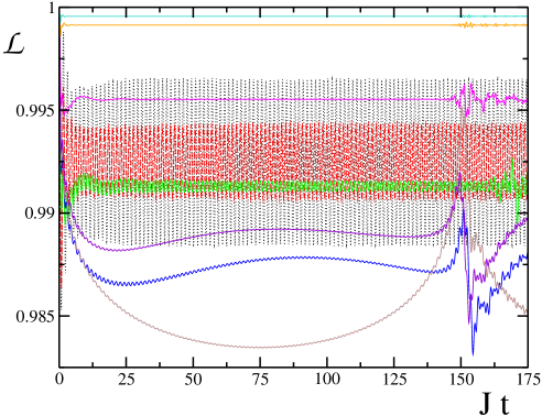
Figure 2: Single-link Ising model ($m=1,\Delta=0,\gamma=1$): Loschmidt echo of Eq. (21) as a function of time for a qubit coupled to a $N=300$ spin chain with periodic boundary conditions (here $\epsilon=0.25$). The various curves are for different values of the transverse magnetic field: $\lambda=$ 0.25 (black dotted), 0.5 (red), 0.9 (green), 0.99 (blue), 1 (brown), 1.01 (violet), 1.1 (magenta), 1.5 (orange), 1.75 (cyan). The critical point corresponds to $\lambda=1$ (brown curve). Notice the revivals of quantum coherence at $t^{*}\sim 150$, due to the finite size of the chain revivals .

IV.1.2 Short-time behavior

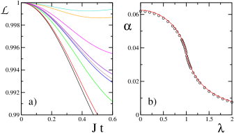
Figure 3: Short-time behavior of the Loschmidt echo: a) magnification of the plot in Fig. 2 for $t\leq 0.6$, where a Gaussian decay $L\sim e^{-\alpha t^{2}}$ is visible; b) dependence of $\alpha$ on $\lambda$ (the solid red line shows the perturbative estimate given by Eq. (26)).

At short times the Loschmidt echo $\mathcal{L}$ decays as a Gaussian peres84 :

$$\mathcal{L}(t)\sim e^{-\alpha t^{2}}\,,$$ (22)

as it can be seen in Fig. 3a, which shows a magnification of the curves from Fig. 2 for small times. This behavior can be predicted within a second-order time perturbation theory in the coupling $\epsilon$ between the system and the bath: if $\epsilon$ is small as compared to the interaction $J$ between neighboring spins in the bath ($\epsilon\ll J$), the decoherence factor $D(t)$ of Eq. (8) can be expanded in series of $\epsilon$:

$$\langle e^{i\mathcal{H}_{g}t}\,e^{-i\mathcal{H}_{e}t}\rangle = \left\langle\mathcal{T}\left[\exp\left(-i\int_{0}^{t}dt^{\prime}e^{i\mathcal{H}_{g}t^{\prime}}\mathcal{W}e^{-i\mathcal{H}_{g}t^{\prime}}\right)\right]\right\rangle$$ (23)

$$\simeq 1+\epsilon\lambda_{1}+\epsilon^{\mathrm{2}}\lambda_{2}\,,$$

where $\mathcal{T}$ is the time ordered product and $\mathcal{W}=\epsilon\,\sigma^{z}_{1}$ accounts for the interaction of the two-level system with the spin chain. The above expression has to be evaluated on the ground state of $\mathcal{H}_{g}$, therefore it is useful to rewrite the interaction $\mathcal{W}$ in terms of the normal mode operators $\eta_{k}^{(g)}$ of $\mathcal{H}_{g}$:

$$\begin{array}[]{rl}\mathcal{W}=&\displaystyle\epsilon\bigg{[}2\sum_{i,j}\big{(}g_{i,1}\eta_{i}^{(g)}{}^{\dagger}+h_{i,1}\eta_{i}^{(g)}\big{)}\cdot\\ {}\hfil&\hskip 29.87547pt\cdot\displaystyle\big{(}g_{j,1}\eta_{j}^{(g)}+h_{j,1}\eta_{j}^{(g)}{}^{\dagger}\big{)}-1\bigg{]}\;.\end{array}$$

The first-order term then reads

$$\lambda_{1}=-it\bigg{(}2\sum_{i}|h_{i,1}|^{2}-1\bigg{)}\,,$$ (24)

while the second-order term is given by

$$\lambda_{2} = -\int_{0}^{t}dt^{\prime}\int_{0}^{t^{\prime}}dt^{\prime\prime}\bigg{[}4\sum_{i\neq j}\Big{(}(g_{i,1}h_{j,1})^{2}$$ (25)

$$- g_{i,1}g_{j,1}h_{i,1}h_{j,1}\Big{)}\,e^{-i(E_{i}+E_{j})(t^{\prime}-t^{\prime\prime})}$$

$$+ \Big{(}2\sum_{i}|h_{i,1}|^{2}-1\Big{)}^{2}\bigg{]}.$$

The Loschmidt echo is then evaluated by taking the square modulus of the decoherence factor:

$$\mathcal{L}(t)\simeq 1-4\epsilon^{2}t^{2}\sum_{i\neq j}\Big{[}(g_{i,1}h_{j,1})^{2}-g_{i,1}g_{j,1}h_{i,1}h_{j,1}\Big{]}\,.$$ (26)

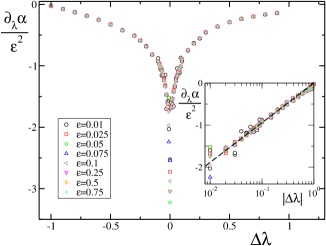
Figure 4: Single-link Ising model ($m=1,\Delta=0,\gamma=1$): Behavior of the Loschmidt echo of Eq. (21) at short times. The plot shows the rescaled parameter $\partial_{\lambda}\alpha/\epsilon^{2}$ as a function of $\lambda$ for a periodic $N=200$ Ising spin chain. Various symbols are for different values of the coupling strength $\epsilon$. Inset: plot in a semi-logarithmic scale. The dashed line indicates a fit of numerical data: $\partial_{\lambda}\alpha/\epsilon^{2}=\tilde{c}_{1}\log|\Delta\lambda|+\tilde{c}_{2}$, with $\tilde{c}_{1}\approx 0.40983$ and $\tilde{c}_{2}\approx 0.000108$.

In Fig. 3b the initial Gaussian rate $\alpha$ is plotted as a function of $\lambda$; circles represent numerical data, while the solid red curve is the perturbative estimate obtained from second-order perturbation theory, given by Eq. (26). In Fig. 4 we analyze the behavior of the first derivative of the rate $\alpha(\lambda,\epsilon)$ as a function of the distance from criticality $\Delta\lambda\equiv\lambda-\lambda_{c}$, for a fixed number $N$ of spins in the chain. As predicted by the perturbative estimate, $\alpha$ scales like $\epsilon^{2}$; most remarkably, its first derivative with respect to the transverse field diverges if the environment is at the critical point $\lambda_{c}$. In the inset we show that $\partial_{\lambda}\alpha$ diverges logarithmically on approaching the critical value, as:

$$\frac{\partial\alpha}{\partial\lambda}=c_{1}\ln|\lambda-\lambda_{c}|+\rm{const.}$$ (27)

This is a universal feature, entirely due to the underlying criticality of the Ising model.

Our results show that at short times the Loschmidt echo is regular even in the presence of a bath undergoing a phase transition. The critical properties of the bath manifest in the changes of ${\cal L}$ when the bath approaches the critical point.

IV.1.3 Long-time behavior

At long times, for $\lambda>1$ the Loschmidt echo approaches an asymptotic value $\mathcal{L}_{\infty}$, while for $\lambda<1$ it oscillates around a constant value (see Fig. 2 for a qualitative picture). This limit value $\mathcal{L}_{\infty}$ strongly depends on $\lambda$ and presents a cusp at the critical point, as shown in Fig. 5.

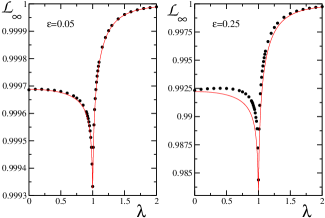
Figure 5: Single-link Ising model ($m=1,\Delta=0,\gamma=1$): Long-time behavior of the Loschmidt echo. The two plots show the saturation value $\mathcal{L}_{\infty}$ as a function of $\lambda$ in an $N=200$ Ising spin chain with periodic b.c., for two different values of the coupling strength: $\epsilon=0.05,\>0.25$. Circles indicate numerical data, solid line is obtained from the perturbative calculation in Eq. (32).

Evidence that $\mathcal{L}_{\infty}$ describes the asymptotic regime can be obtained by comparing data with the result of an analytical expression based on the following simple ansatz: We assume that at the thermodynamic limit $N\to\infty$ the coherence loss saturates and is constant after a given transient time $t_{0}$

$$\mathcal{L}\approx\mathcal{L}_{\infty}\qquad\forall\>t\geq t_{0}.$$ (28)

By writing the ground state $\left|G\right\rangle$ of $\mathcal{H}_{g}$ on the eigenbasis of $\mathcal{H}_{e}$, the Loschmidt echo in Eq. (9) can be formally written as

$$\mathcal{L}=\Big{|}\sum_{k}|c_{k}|^{2}e^{-i\,E_{k}^{(e)}t}\Big{|}^{2}\;.$$ (29)

Here, $c_{k}$ are the coefficients of the expansion $|\psi_{0}^{(g)}\rangle=\sum_{k}c_{k}\,|\psi_{k}^{(e)}\rangle$, where $\mathcal{H}_{e}|\psi_{k}^{(e)}\rangle=E_{k}^{(e)}|\psi_{k}^{(e)}\rangle$ and $|\psi_{0}^{(g)}\rangle\equiv\left|G\right\rangle$. An integration of the ansatz Eq. (28) from time $T>t_{0}$ to time $T+\Delta$ thus gives:

$$\mathcal{L}_{\infty}=\left|\sum_{k}|c_{k}|^{2}e^{-iE_{k}^{(e)}\left(T+\frac{\Delta}{2}\right)}\>\textrm{sinc}\Big{(}\frac{E_{k}^{(e)}\Delta}{2}\Big{)}\right|^{2}\,,$$ (30)

where $\textrm{sinc}\,(x)=\sin(x)/x$. If the ground state in the perturbed Hamiltonian $\mathcal{H}_{e}$ is not degenerate, we can just retain the term in the sum corresponding to $k=0$, thus obtaining $\mathcal{L}_{\infty}\approx|c_{0}|^{4}$. Therefore a rough estimate of the Loschmidt echo is given by the overlap between the ground state of $\mathcal{H}_{g}$ and the ground state of $\mathcal{H}_{e}$ (see Ref. zanardi06 for a detailed analysis of the ground state fidelity in spin systems). This can be evaluated via second-order perturbation theory in $\epsilon$:

$$c_{0}=1-\frac{1}{2}\sum_{k\neq 0}\frac{\left|\langle\psi_{k}^{(g)}|\,\mathcal{W}\,|\psi_{0}^{(g)}\rangle\right|^{2}}{\left(E_{k}^{(g)}-E_{0}^{(g)}\right)^{2}}$$ (31)

where $|\psi_{k}^{(g)}\rangle$ are the excited states of $\mathcal{H}_{g}$ with energies $E_{k}^{(g)}$ and $\mathcal{W}=\epsilon\sum_{j=j_{1}}^{j_{m}}\sigma^{z}_{1}$. The expression in Eq. (31) can be easily computed for the case $m=1$ following the same steps used to evaluate Eq. (23). The final result is:

$$\mathcal{L}_{\infty}\approx\Bigg{[}1-2\epsilon^{2}\sum_{i\neq j}\bigg{(}\frac{g_{i1}\,h_{j1}}{\tilde{E}_{i}^{(g)}+\tilde{E}_{j}^{(g)}}\bigg{)}^{2}\,\Bigg{]}^{4},$$ (32)

where the energies $\tilde{E}_{k}^{(g)}$ are rescaled on the ground state energy, $\tilde{E}_{k}^{(g)}=E_{k}^{(g)}-E_{0}^{(g)}$. In Fig. 5 we plotted these results for two different values of the perturbation strength (solid lines); they can be compared with the exact numerical results (circles). Notice that analytic estimates are more accurate for small $\epsilon$, and far from the critical region.

IV.1.4 Ising bath: scaling with the size

As one could expect, contrary to the case of a non-local system-bath coupling quan , if the environment is not at the critical point, the decay of the coherences is independent of the number of spins in the bath. This is due to the fact that correlations away from criticality decay exponentially, while they decay as a power law at the critical point. In particular, we checked that both the initial rate $\alpha$ and the saturation value $\mathcal{L}_{\infty}$ do not depend significantly on $N$ for $\lambda\neq\lambda_{c}$. We present here a simple argument as a confirmation of this statement. Far from the critical region, independently of the bath size (for sufficiently large baths), a qubit simultaneously coupled to two non-communicating $N$-sites chains via a one-spin link (configuration 1) should decohere in the same way as if it was coupled to two sufficiently distant spins of a $2N$-sites chain (configuration 2). A pictorial representation of the two configurations described above is shown in Fig. 6, where the red spin represents the system, the grey ones are the bath spins directly coupled to the system.

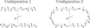
Figure 6: Qubit (red) coupled to two non-communicating $N$-sites chains (configuration 1) and to two spins of a $2N$-sites chain (configuration 2). Here, as an example, we set $N=11$.

We numerically checked that, far from the critical region, the two configurations leave the decoherence unchanged. In particular we chose an $N=200$ chain, and obtained that, if $|\lambda-\lambda_{c}|\gtrsim 10^{-2}$, the Loschmidt echo evaluated in the two configurations is the same, up to a discrepancy of $10^{-5}$, as it can be seen from Fig. 7.

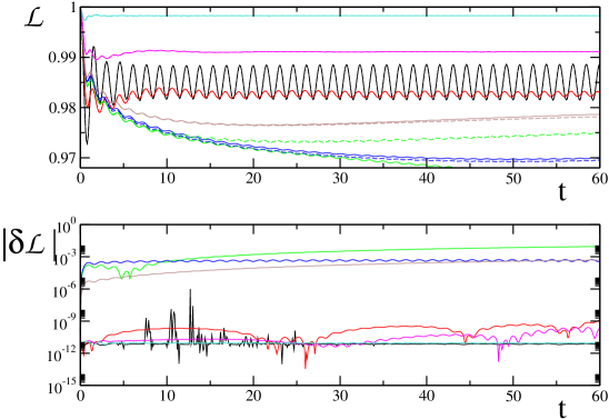
Figure 7: Upper figure: solid curves stand for the qubit coupled to two non communicating open $N=200$ spin Ising chains (configuration 1); dashed curves are for the qubit coupled to two opposite spins of a periodic $N=400$ spin Ising chain (configuration 2). Different curves are for various values of the transverse magnetic field: $\lambda=0.5$ (black), 0.9 (red), 0.99 (green), 1 (blue), 1.01 (brown), 1.1 (magenta), 1.5 (cyan). Lower figure: absolute differences between the two configurations.

At the critical point instead the behavior dramatically changes. In Fig. 8 we plot the decay of $\mathcal{L}$ in time at $\lambda_{c}$ for different sizes of the chain and fixed perturbation strength, $\epsilon=0.25$. The minimum value $\mathcal{L}_{0}^{c}$ reached by the Loschmidt echo decays with the size $N$ as

$$\mathcal{L}_{0}^{c}=\frac{\mathcal{L}_{0}}{1+\beta\ln(N)}.$$ (33)

Notice also that revivals are due to the finiteness of the environmental size (as in Fig. 2) revivals . We expect that the coherence loss should go to zero at the thermodynamic limit $N\to\infty$; this is hard to see numerically, since the decay is logarithmic, and the actual value of $\mathcal{L}_{0}^{c}$ is still quite far from zero, even for $N=2000$ spins.

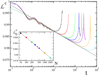
Figure 8: Single-link Ising model ($m=1,\Delta=0,\gamma=1$). Loschmidt echo as a function of time at the critical point $\lambda=1$, for different sizes of the periodic chain: $N=50$ (black), 100 (red), 200 (green), 300 (blue), 400 (brown), 500 (violet), 1000 (orange), 2000 (cyan). The perturbation strength is kept fixed: $\epsilon=0.25$. The dashed line is a guideline that shows a decay of the type $\mathcal{L}^{c}(t)=c_{0}/(1+c_{1}\,\textrm{ln}\,t)$. Inset: Minimum value of $\mathcal{L}^{c}$ as a function of $N$. Numerical data have been fitted with $\mathcal{L}_{0}^{c}=\mathcal{L}_{0}/(1+\beta\,\textrm{ln}N)$ (dot-dashed line), where $\mathcal{L}_{0}\approx 0.99671,\;\beta\approx 2.36933\times 10^{-3}$.

IV.1.5 $XY$-baths with arbitrary $xy$-anisotropy $\gamma$

The properties described in the previous Subsections are typical of the Ising universality class, indeed they remain qualitatively the same as far as $\Delta=0,\gamma\neq 0$ in Eq. (3): in particular this class of models has one critical point at $\lambda=1$. Following our previous analysis of the Ising model ($\gamma=1$), we focus on the two distinct regions of short- and long-time behavior, whose features are depicted in Fig. 9.

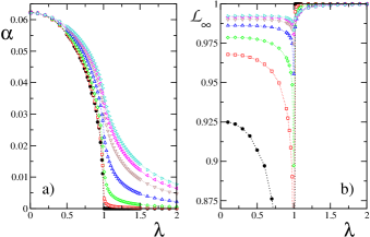
Figure 9: Single-link $XY$-models ($m=1,\Delta=0$): Short- and long-time behavior of the Loschmidt echo for a qubit coupled to a periodic $N=300$ spin $XY$ chain, with a coupling strength $\epsilon=0.25$. a) Small times (initial Gaussian decay rate $\alpha$); b) Long times (saturation values ${\cal L}_{\infty}$). The various curves are for different anisotropy values: $\gamma=$ 0 ($XX$-model, full black circles), 0.1 (red squares), 0.25 (green diamonds), 0.5 (blue triangles up), 0.75 (brown triangles down), 0.9 (magenta triangles left), 1 (Ising, cyan triangles right).

At small times the decay is again Gaussian, as in Eq. (22), and the first derivative of the decay rate $\alpha$ with respect to $\lambda$ diverges at $\lambda_{c}$ (see Fig 9a). As far as the $xy$ anisotropy decreases, the system approaches a limiting case in which $\partial_{\lambda}^{-}\alpha=-\infty$, while $\partial_{\lambda}^{+}\alpha=0$. The asymptotic value $\mathcal{L}_{\infty}$ at long times shows a cusp at $\lambda=1$; notice that, as the anisotropy $\gamma$ decreases, despite the fact that the decay of coherences at short times is always reduced, their saturation value $\mathcal{L}_{\infty}$ becomes lower for $\lambda<1$, while gets higher for $\lambda>1$. Therefore decoherence is asymptotically suppressed only in the ferromagnetic phase, while it is enhanced for $\lambda<1$. As we said before, when $\gamma\to 0$ the system is driven towards a discontinuity at $\lambda=1$. This is due to the fact that for $\lambda>1$ the ground state approaches a fully polarized ferromagnetic state. Finally we analyzed the scaling of the decoherence with the size of the environment at criticality. As in the Ising model, the minimum value $\mathcal{L}_{0}^{c}$ reached by the Loschmidt echo at $\lambda_{c}$ depends on the chain length $N$ as in Eq. (33): $\mathcal{L}_{0}^{c}=\mathcal{L}_{0}/(1+\beta\ln(N))$.

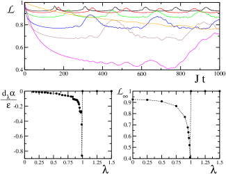
Figure 10: Single-link $XX$-model ($m=1,\Delta=\gamma=0$): Temporal behavior of the Loschmidt echo for a qubit coupled to a periodic $N=300$ spin isotropic $XX$ chain; $\epsilon=0.25$. The various curves stand for different values of the magnetic field: $\lambda=$ 0.25 (black), 0.5 (red), 0.75 (green), 0.9 (blue), 0.95 (brown), 0.99 (magenta), 1. (orange). Bottom left: first derivative of the decay rate $\alpha$ at short times with respect to $\lambda$, as a function of $\lambda$. Bottom right: saturation value $\mathcal{L}_{\infty}$ at long times.

The system behaviour dramatically changes when it becomes isotropic, i.e. at $\gamma=0$. In this case the environment is an $XX$ spin chain and it does not belong any more to the Ising universality class. In particular it exhibits a critical behavior over the whole parameter range $|\lambda|\leq 1$, while it is ferromagnetic (anti-ferromagnetic) for $\lambda>1$ ($\lambda<-1$). The decay of the Loschmidt echo (shown in Fig. 10) reflects its critical properties: indeed we found that it behaves as in Eq. (33) over the whole range $|\lambda|\leq 1$. In the ferromagnetic case instead the coupled qubit does not decohere at all (i.e. $\mathcal{L}(t)=1$), since the ground state of the $XX$-model for $\lambda>1$ is the fully polarized state with all spins parallel to the external field. The first derivative of the initial decay rate $\partial_{\lambda}\alpha$ is monotonically negative in the critical region by increasing $\lambda$ and diverges for $\lambda\to 1^{-}$, while it is strictly zero for $\lambda>1$. Also the plateau $\mathcal{L}_{\infty}$ as a function of $\lambda$ presents a discontinuity in $\lambda=1$, since it drops to zero for $\lambda\to 1^{-}$, and it equals one for $\lambda>1$.

IV.2 $XXZ$-Heisenberg chain bath

In this Section we consider a single-link ($m=1$) $XXZ$ anisotropic Heisenberg chain ($\lambda=\gamma=0$ in Eq. (3)) with anisotropy parameter $\Delta$. We resort to the numerical t-DMRG to compute the Loschmidt echo (9), since this specific spin model is not integrable. A brief introduction to the static and the time-dependent DMRG algorithm is given in Appendix A. We consider open boundary conditions, since DMRG with periodic boundaries intrinsically gives much less accurate results schollwock . The evaluation of the Loschmidt echo with the t-DRMG is more time- and memory-consuming than its exact calculation in the solvable cases, therefore at present we could not study the behavior of $\mathcal{L}(t)$ at long times. Nonetheless we are able to fully analyze the short-time behavior in systems with environment size of up to $N\sim 10^{2}$ spins. In the following we show the results concerning the coupling of the two-level system to one spin in the middle of the chain: this corresponds to the case with less border effects. We numerically checked that the results are not qualitatively affected from this choice, but changing the system-environment link position results in a faster appearance of finite size effects due to the open boundaries.

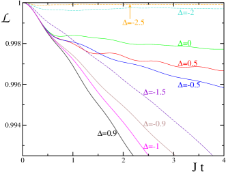
Figure 11: Single-link $XXZ$-model ($m=1,\lambda=\gamma=0$): Loschmidt echo as a function of time for a qubit coupled to the central spin of an open ended $N=100$ spin $XXZ$-Heisenberg chain, with coupling strength $\epsilon=0.1$. The various curves are for different values of the anisotropy: $\Delta=0.9$ (black), 0.5 (red), 0 (green), -0.5 (blue), -0.9 (brown), -1 (magenta), -1.5 (violet), -2 (cyan), -2.5 (orange); curves corresponding to non-critical situations are dashed.

In Fig. 11 we plot the decay of the Loschmidt echo as a function of time, for various values of the anisotropy $\Delta$ and fixed coupling strength $\epsilon=0.1$. In the ferromagnetic zone outside of the critical region ($\Delta\geq 1$) $\mathcal{L}$ does not decay at all, as a consequence of the ground state full polarization. In the critical region and for long times, the Loschmidt echo decay is proportional to the modulus of $\Delta$ and for $\Delta>-1$ it slows down until it is completely suppressed in the perfectly anti-ferromagnetic regime ($\Delta\to-\infty$). The short time decay is again Gaussian at short times and the rate $\alpha$ is shown in Fig. 12 for various sizes of the bath. We notice two qualitatively different behaviors at the boundaries of the critical region: at $\Delta=+1$ there is a sharp discontinuity, while at $\Delta=-1$ the curve is continuous. In the critical region $-1\leq\Delta\leq 1$ the initial decay rate $\alpha$ is constant and reaches its maximum value due to the presence of low energy modes, while in the ferromagnetic phase $\Delta\geq 1$ it is strictly zero. In the figure, finite size effects are evident: indeed, contrary to the $XY$-model, the decay rate $\alpha$ changes with the bath size $N$ outside the critical region. However, as the system approaches the thermodynamic limit ($N\to\infty$), the dependence on $N$ weakens and, while at $\Delta=-1$ the curve $\alpha(\Delta)$ appears to remain continuous, its first derivative with respect to $\Delta$ tends to diverge. On the contrary, the ferromagnetic transition $\Delta=1$ is discontinuous independently of $N$.

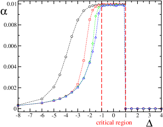
Figure 12: Scaling of the decay rate $\alpha$ at short times for an open ended $XXZ$-Heisenberg chain as a function of $\Delta$. The various symbols are for different sizes of the chain: $N=10$ (black circles), 20 (red squares), 50 (green diamonds), 100 (blue triangles). The coupling strength between the qubit and the chain is kept fixed at $\epsilon=0.1$.

IV.3 Decoherence and entanglement

We propose here to establish a link between decoherence effects on the system and entanglement inside the environment. This study can be justified by the fact that decoherence properties of the qubit system seem to be intrinsically related to quantum correlations of the bath, as the proximity to critical points reveals. On the other hand, entanglement quantifies the amount of these correlations that do not have classical counterparts, and it has been widely studied in the recent years, especially in connection with the onset of quantum phase transitions osterloh02 ; osborne02 ; vidal03 ; stauber04 .

In Ref. dawson it was shown that two-party entanglement in the environmental bath of a central spin model can suppress decoherence; this effect has been explained as a consequence of entanglement sharing, and it was supposed to be common to any system whose environment maintains appreciable internal entanglement, while evolving in time. We now characterize a more complex case of system-plus-bath coupling, given by Eq. (1), with a richer structure in the ground state entanglement which suggests the following picture, valid at short times for $Jt\ll 1$.

We expect that when the decay of coherences is quadratic, only short range correlations in the bath are important, therefore it seems natural to relate the short-time decay rate $\alpha$ to the two-site nearest neighbor entanglement of the chain. All the information needed to analyze bipartite entanglement between two spins inside the chain, say $i$ and $j$, is contained in the two-qubit reduced density matrix $\rho_{ij}$, obtained after tracing out all the other spins. We use the concurrence $C(|i-j|)$ as an entanglement measure for arbitrary mixed state $\rho_{ij}$ of two qubits defined as wootters

$$C(|i-j|)=\max(\lambda_{1}-\lambda_{2}-\lambda_{3}-\lambda_{4},0),$$ (34)

where $\lambda_{1}$ are the square roots of the eigenvalues of the matrix $\rho_{ij}\tilde{\rho}_{ij}$, in decreasing order; the spin flipped matrix of $\rho_{ij}$ is defined as $\tilde{\rho}_{ij}=(\sigma_{y}\otimes\sigma_{y})\,\rho^{*}_{ij}\,(\sigma_{y}\otimes\sigma_{y})$, and the complex conjugate is computed in the canonical basis $\{|\uparrow\uparrow\rangle,|\uparrow\downarrow\rangle,|\downarrow\uparrow\rangle,|\downarrow\downarrow\rangle\}$ . The entanglement of formation of the mixed state $\rho_{ij}$ is a monotonic function of the concurrence.

We start our analysis by considering again the $XY$ spin bath: the concurrence $C(k)$ in terms of one-point and two-point spin-correlation functions can be analytically evaluated amico04 ; barouch . As long as $\gamma\neq 0$, this system belongs to the Ising universality class, for which it has been shown that the concurrence between two spins vanishes unless the two sites are at most next-to-nearest neighbor osterloh02 ; osborne02 . The nearest-neighbor concurrence $C(1)$ presents a maximum that occurs at $\lambda=\lambda_{m}>1$, and it is not related to the critical properties of the model. For $\lambda>\lambda_{m}$ it monotonically decreases to zero, as the ground state goes towards the ferromagnetic product state. For $\lambda<\lambda_{m}$ the concurrence decreases and precisely reaches zero at $\lambda_{K}=\sqrt{(1+\gamma)(1-\gamma)}$, where the ground state exactly factorizes kurmann .

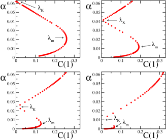
Figure 13: Dependence of the Loschmidt echo decay rate $\alpha$ on the nearest-neighbor concurrence $C(1)$ in the $XY$-model, for $\epsilon=0.25$ and different anisotropy values: $\gamma=1$ (upper left), 0.5 (upper right), 0.25 (lower left), 0.1 (lower right). Data have been evaluated for an $N=301$ spin chain.

In the proximity of the quantum phase transition, the entanglement obeys a scaling behavior osterloh02 ; in particular at the thermodynamic limit the critical point is characterized by a logarithmic divergence of the first derivative of the concurrence: $\partial_{\lambda}C(1)\sim\ln|\lambda-\lambda_{c}|$. A similar divergence has been found for the first derivative of the decay rate $\alpha$ of the Loschmidt echo (see the inset of Fig. 4). In Fig. 13 we analyzed the dependence of $\alpha$ as a function of the nearest-neighbor concurrence $C(1)$. The behavior $\alpha(C)$ is not monotonic, since $\alpha$ monotonically decreases with $\lambda$ (see Fig. 3b), while $C(1)$ has a non-monotonic behavior. Indeed, for $\lambda>\lambda_{m}$ and $\lambda<\lambda_{K}$ the two quantities are correlated, while they are anti-correlated for $\lambda_{m}>\lambda>\lambda_{K}$.

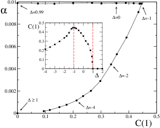
Figure 14: Decay rate $\alpha$ as a function of the nearest-neighbor concurrence $C(1)$ in the Heisenberg model for $N=100$, $\epsilon=0.1$. Inset: nearest-neighbor concurrence as a function of the anisotropy $\Delta$. The two dashed lines isolate the critical region.

A similar scenario has been found in the case of the Heisenberg chain as a spin bath, reported in Fig. 14. As for the Ising model, the behavior of $\alpha(C)$ is not monotonic, following the concurrence behavior: Indeed $C(1)$ is zero for $\Delta\geq 1$ (in the fully polarized ground state), it monotonically increases while decreasing $\Delta$ up to $\Delta=-1$, and then starts to decrease again, vanishing in the perfect anti-ferromagnetic limit $\Delta\to-\infty$ syljuasen . In conclusion, the behavior $\alpha=\alpha(C)$ is monotonically increasing in the anti-ferromagnetic region, is constant at the criticality, and is strictly zero for the ferromagnetic phase (see Figs. 11b, 12), resulting in a direct correlation of $\alpha$ and $C(1)$ in the anti-ferromagnetic phase.

V Results: the multiple-links scenario

In this Section we study the case in which the system $S$ is non-locally coupled to more than one spin of the bath $E$, namely we choose $m\neq 1$ in the interaction Hamiltonian Eq. (4). In general, given a number $m$ of links, there are many different ways to couple the two-level system with the bath spins. In the following we will consider two geometrically different setups: a spin-symmetric configuration (type A) where the qubit is linked to some spins of the chain which are equally spaced, and a non-symmetric configuration (type B) where the spins to which the qubit is linked are nearest neighbor. We will also suppose that the interaction strength $\epsilon$ between the qubit and each spin of the bath is kept fixed and equal for all the links. A schematic picture of the two configurations is given in Fig. 15. We will present results concerning an environment constituted by an Ising spin chain with periodic boundary conditions. Notice that this system-environment coupling can induce the emergence of criticality in $E$ even for small couping $\epsilon\ll J$ in the central spin scheme, i.e. $m=N$ quan ; cucchietti2 ; ou06 . Indeed, in this case, a perturbation $\epsilon$ results in a change of the external magnetic field of the chain from $\lambda$ to $\lambda+\epsilon$. If the environment is characterized by $\lambda<1$, at $\epsilon>1-\lambda$ the coupling drives a quantum phase transition in the bath cucchietti2 .

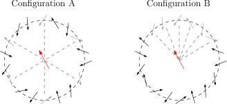
Figure 15: Different setups for the coupling of the two-level system (red spin) with the spin chain. The qubit is linked to the spins of the chain depicted in grey. Configuration A shows a star-symmetric setup, while configuration B is a non-symmetric packed setup. As a pictorial example, here we set $N=18,\,m=6$.

V.0.1 Short-time behavior

At short times the Loschmidt echo exhibits a Gaussian decay, as in Eq. (22), for both configurations. For the setup A the decay rate $\alpha$, far from the critical region, scales as

$$\alpha\propto m\,\epsilon^{2},$$ (35)

as it can be seen from Fig. 16a. The scaling with the number of links $m$ is a consequence of the fact that the short-time behavior is dominated by the dynamics of the environment spins close to those linked to the qubit (see also Sec. IV.3). Therefore, if the linked spins are not close to each other, they do not interact among them on the short time scale $Jt\ll 1$. Near the critical point this picture is not valid, since long-range correlations between the spins of the bath become important, even at small times. In this region indeed the scaling $\alpha\sim m$ is less appropriate, as it can be seen in the inset of Fig 16a.

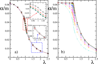
Figure 16: Decay rate $\alpha$ rescaled with respect to the number of links $m$, in a star symmetric configuration (type A) on the left, and in a non-symmetric configuration (type B) on the right. The environment is an $N=300$ spin Ising chain with periodic boundary conditions. The interaction strength $\epsilon$ is kept fixed for all the links between the qubit and the environment spins: $\epsilon=0.25$. Various symbols stand for different values of $m$: 1 (plus), 2 (triangles right), 3 (triangles down), 5 (triangles left), 10 (triangles up), 30 (diamonds), 100 (squares), 150 (circles), 300 (dashed line, right figure). The inset on the left figure shows a magnification of the same plot, centered in proximity of the critical point $\lambda_{c}=1$.

The scaling of Eq.(35) does not hold any more in the setup B, as in this case collective modes influence the dynamics of the system even at short times, since the spins linked to the central spin are close to each other and they are not independent any more. This is clearly visible in Fig. 16b. We notice also that, as $m/N$ increases, $\alpha$ tends to remain constant for $\lambda\leq 1$ and then decreases for $\lambda>1$. In the limiting case $m=N$, $\alpha$ is positive and strictly constant for $\lambda\leq\lambda_{c}$; the first derivative $\partial_{\lambda}\alpha$ presents a discontinuity at $\lambda_{c}$, showing a divergence from the ferromagnetic zone $\lambda\to 1^{+}$.

V.0.2 Long-time behavior

In this Section we concentrate on the setup B, since the configuration A is less interesting: indeed for long times the Loschmidt echo behaves as if the qubit was coupled to an environment with a smaller number of spins. In Fig. 17 we plotted the asymptotic value of the Loschmidt echo $\mathcal{L}_{\infty}$ for the setup B. We observe that, as $m$ increases, the coherence loss enhances, and the valley around the critical point $\lambda_{c}$ deepens and gets broader. Notice also that, when approaching the central spin limit, the asymptotic value $\mathcal{L}_{\infty}$ reaches values very close to zero, even far from criticality. This situation is completely different from what occurs in the single-link scenario where, away from criticality, the Loschmidt echo remains very close to one even for non negligible system-bath coupling strengths (e.g., for $\epsilon=J/4$ we found $\mathcal{L}_{\infty}\sim 0.99$, as it can be seen, for example, from Figs. 2, 5).

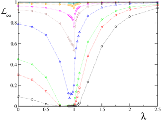
Figure 17: Asymptotic value of the Loschmidt echo for the setup B; the environment is a 300 spin Ising chain, with $\epsilon=0.25$. Various symbols stand for different values of $m$: 1 (plus), 2 (triangles right), 5 (triangles down), 10 (triangles left), 30 (triangles up), 100 (diamonds), 150 (squares), 300 (circles).

V.1 Strong coupling to the bath

Under certain conditions decoherence induced by the coupling with a bath manifests universal features: In Refs. cucchietti2 ; zurek3 it has been shown that when the coupling to the system drives a quantum phase transition in the environment, the decay of coherences in the system is Gaussian in time, with a width independent of the coupling strength. In particular, for a central spin coupled to an $N$-spin Ising chain, the Loschmidt echo in Eq. (51) is characterized by a Gaussian envelope modulating an oscillating term:

$$\mathcal{L}(t)=|\cos(\epsilon t)|^{N/2}\>e^{-S_{N}^{2}t^{2}}\,,$$ (36)

provided that

$$\lambda<1\qquad{\rm and}\quad\lambda+\epsilon\gg 1\,.$$ (37)

The oscillations are not universal, but the Gaussian width $S_{N}^{2}$ depends only on the properties of the environment Hamiltonian, in particular it is independent of the coupling strength $\epsilon$ and of the transverse magnetic field $\lambda$, while it is proportional to the number $N$ of spins in the bath. The case of the central spin model is illustrated in Fig. 18a, where the different curves stand for various values of $\epsilon$.

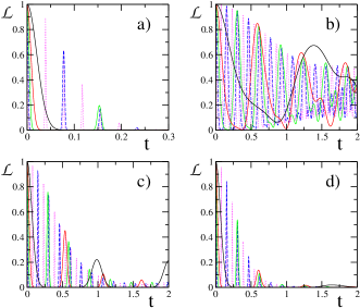
Figure 18: Loschmidt echo for the Ising model with $N=300$ spins as environment, $\lambda=0.5$. The various panels are for different numbers of spins $m$ coupled to the qubit system and for various geometries: a) $m=300$ (central spin system); b) $m=3$, configuration B; c) $m=30$, configuration A; d) $m=30$, configuration B. Different curves correspond to various values of the coupling strength: $\epsilon=2$ (full black), 5 (full red), 10 (full green), 20 (dashed blue), 40 (dotted magenta).

This universal behavior for strong couplings is present in more general qubit-environment coupling, different from the central spin limit, provided that the same conditions in Eq. (37) on $\lambda$ and $\epsilon$ hold. In the Ising bath model, we checked that it remains valid also for a number of system-bath links $m\neq N$ and for different geometries, as it can be seen in Fig. 18 (panels b-d). The fast oscillations remain proportional to $\epsilon$, since they are a consequence of the interaction $\propto\epsilon\,\tau_{z}\sigma^{z}_{j}$ between the qubit and the spins of the bath. Instead in general the envelope is Gaussian only for small times, but its width $S_{N}^{2}$ is independent of $\epsilon$.

We found that, for the non-symmetric configuration B, $S_{N}^{2}$ depends only on the number of links $m$, being proportional to it. No dependence from the perturbation strength $\epsilon$, the size $N$ of the bath, or the transverse magnetic field $\lambda$ has been observed, provided that $m\gtrsim 10$, as it can be seen from Fig. 19b. Indeed in the setup B the qubit behaves like in the central spin model: in the regime of strong coupling, the effect of the environment spins not directly linked to the qubit can be neglected since they interact weakly, as compared to the system-bath interactions. Therefore a system strongly coupled to $m$ neighbour spins of an $N$-spin chain decoheres in the same way as if it was coupled to all the spins of an $m$-spin chain.

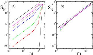
Figure 19: Width of the Gaussian envelope $S_{N}^{2}$ as a function of the number of links $m$ between the system and the bath, for different values of the transverse magnetic field: $\lambda=0$ (circles), 0.1 (squares), 0.2 (diamonds), 0.5 (triangles up), 0.7 (triangles down), 0.9 (triangles left). The bath is modeled as an $N=200$ Ising chain with periodic boundary conditions; the coupling strength is kept fixed and equal to $\epsilon=80$. The two panels correspond to: a) star-symmetric configuration (type A); b) non-symmetric configuration (type B). Dashed black curves represent a linear behavior $S_{N}^{2}\sim m$ and are plotted as guidelines.

The decoherence effects are richer in the geometry A. In this setup the effect of the spins not directly coupled to the qubit cannot be ignored, indeed we found that $S^{2}_{N}$ depends on the internal dynamics of the bath. In particular we found that

$$S_{N}^{2}\sim m\,\lambda^{2}\,,$$ (38)

where $\lambda$ is the transverse magnetic field (see Fig. 19a and Fig. 20). Notice that, as it can be seen from Fig. 19a, the case $\lambda=0$ is rather peculiar, since the system does not decohere at all, unless it is uniformly coupled to all the spins of the environment. This is due to the fact that an Ising chain in the absence of a transverse field is not capable of transmitting quantum information: in this system the density matrix of two non-neighbouring spins evolves independently of the other spins.

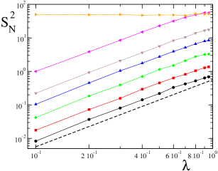
Figure 20: $S_{N}^{2}$ as a function of the transverse field $\lambda$ in an $N=200$ spin Ising bath, for different numbers of system-bath links in the configuration A: $m=$ 2 (circles), 4 (squares), 10 (diamonds), 25 (triangles up), 50 (triangles down), 100 (triangles left), 200 (triangles right). The coupling strength is kept fixed and equal to $\epsilon=80$. The case $m=200$ (triangles right) corresponds to the central spin model.

VI Conclusions

In this work we analyzed a model of environment constituted by an interacting one-dimensional quantum spin-1/2 chain. We have shown that this type of baths can be experimentally engineered in a fully controllable and tunable way by means of optical lattices, and we provided a detailed description of the pulse sequence needed to realize a pure dephasing model for a qubit system coupled to a spin bath. The open quantum system model we proposed here is simpler to implement in an experimental setup, with respect to the widely studied central spin model in which the system is uniformly coupled to all the spins of the environment. Nonetheless, we have analyzed the crossover from the single link to the central spin model by taking in account different geometries and different number of links, recovering, in the central spin limit, known results present in literature, and characterizing new behaviors in between.

The coherence loss in the system has been quantified by means of the Loschmidt echo; the rich structure of the environment baths allowed us to analyze the impact of the different phases and of the distance from criticality, and more generally to study the connection between entanglement inside the bath and decoherence effects in the system.

First we considered the case of one link between the qubit and the chain. We showed that at short times the Loschmidt echo decays as a Gaussian, while for long times it approaches an asymptotic value which strongly depends on the transverse field strength. Criticality emerges in both short- and long-time behaviors: the $XY$ spin bath is characterized by the first derivative of the Gaussian width with respect to the field strength that diverges logarithmically at $\lambda_{c}$, while the saturation values of the Loschmidt echo at long times exhibits a sharp cusp in correspondence to the critical point. The decay rate at short times due to a Heisenberg spin bath is maximum and constant throughout the whole critical region. We also showed that, contrary to the central spin model, if the environment is not critical, the decay of coherences in the system is independent of the bath size. Subsequently we related decoherence properties of the system with quantum correlations inside the environment: we studied the Gaussian decay rate at short times as a function of the concurrence of two nearest neighbor spins in the bath. We then analyzed a non-local system-bath coupling in which the qubit is connected to the chain with multiple links, by considering two different setups: a spin-symmetric and a non-symmetric one. Finally we reported the existence of a coupling-independent regime, with the only hypothesis of having a strong system-bath coupling.

Appendix A DMRG approach

An analytic solution for a spin coupled to a Heisenberg $XXZ$-model (i.e. $\{\Delta\neq 0$, $\lambda=0\}$ in Eq. (3)) is not available, therefore a numerical approach is required. We resort to the recently developed time-dependent Density Matrix Renormalization Group (t-DMRG) with open boundary conditions white92 ; white04 ; schollwock ; dmrgreview ), in order to calculate the overlap between the ground state $\left|G\right\rangle$ of $\mathcal{H}_{g}$ and the time evolution of the same state under the Hamiltonian $\mathcal{H}_{e}$ (see Eq. (9)).

First, the static DMRG algorithm allows us to evaluate the ground state $\left|G\right\rangle$ of $\mathcal{H}_{g}$. This algorithm in its first formulation white92 is an iterative numerical technique to find the ground state of a one-dimensional system constituted by sites which possess local and nearest-neighbor couplings, therefore it is well suited for systems like the Hamiltonian in Eq. (3). The key strategy of the DMRG is to construct a portion of the system, called the system block, and then recursively enlarge it, until the desired size is reached. At every step the basis of the corresponding Hamiltonian is truncated, so that the size of the Hilbert space remains manageable as the physical system grows. The truncation of the Hilbert space is performed by retaining the eigenstates corresponding to the $D$ highest eigenvalues of the block’s reduced density matrix.

The t-DMRG is then subsequently used, in order to simulate the dynamics of $\left|G\right\rangle$ under the Hamiltonian $\mathcal{H}_{e}$. The t-DMRG algorithm white04 is an extension of the static DMRG, which follows the dynamics of a certain state $\left|\psi\right\rangle$ under the Hamiltonian $\mathcal{H}$ of a nearest-neighbor one-dimensional system. The time evolution can be implemented by using a second-order Suzuki-Trotter decomposition white04 of the time evolution operator $U=e^{-i\mathcal{H}_{e}t}$:

$$e^{-i\mathcal{H}_{e}t}\approx\left(e^{-i\mathcal{F}\frac{\delta t}{2}}e^{-i\mathcal{G}\delta t}e^{-i\mathcal{F}\frac{\delta t}{2}}\right)^{n}\,.$$ (39)

Here we have first written the Hamiltonian as $\mathcal{H}_{e}=\mathcal{F}+\mathcal{G}$ where $\mathcal{F}$ contains the on-site terms and the even bonds while $\mathcal{G}$ is formed by the odd bonds; $n=t/\delta t$ is the time expressed in number of trotter steps. We also keep track of the state $\left|G\right\rangle$ in the new truncated basis of $e^{-i\mathcal{H}_{e}t}\left|G\right\rangle$, so that we can straightforwardly evaluate the overlap in Eq. (9). During the evolution the wave function is changing, therefore the truncated basis chosen to represent the initial state has to be updated by repeating the DMRG renormalization procedure using the instantaneous state as the target state for the reduced density matrix.

The results presented in this paper concerning Heisenberg spin baths, have been obtained by performing time evolution within a second order Trotter expansion, with a Trotter slicing $J\,\delta t=10^{-3}$ and a truncated Hilbert space of dimension $D=100$. The evaluation of the Loschmidt echo with the t-DMRG is much more time- and memory-expensive than the analytical approach of Eq. (21), limiting the bath size in our simulations up to $N\sim 10^{2}$ spins.

Appendix B Fermion correlation functions

We provide an explicit expression for the two-point correlation matrix $({\bf r})_{ij}=\langle\Psi^{\dagger}_{i}\Psi_{j}\rangle$ of the operators ${\bf\Psi^{\dagger}}=\big{(}c_{1}^{\dagger}\ldots c_{N}^{\dagger}\,c_{1}\ldots c_{N}\big{)}$ on the ground state of the system Hamiltonian $\mathcal{H}_{g}$. The $2N\times 2N$ matrix r is written in terms of the Jordan Wigner fermions $\{c_{k},c_{k}^{\dagger}\}$ as:

$${\bf r}=\left(\begin{array}[]{cc}\big{<}c^{\dagger}_{i}c_{j}\big{>}_{i,j=1,N}&\big{<}c^{\dagger}_{i}c^{\dagger}_{j}\big{>}_{i,j=1,N}\\ \big{<}c_{i}c_{j}\big{>}_{i,j=1,N}&\big{<}c_{i}c^{\dagger}_{j}\big{>}_{i,j=1,N}\end{array}\right)\,.$$ (40)

Therefore it is sufficient to express $\{c_{k},c_{k}^{\dagger}\}$ in terms of the normal mode operators $\{\eta_{k}^{(g)},\eta_{k}^{(g)\dagger}\}$ which diagonalize the Hamiltonian $\mathcal{H}_{g}$, since $<\eta_{j}^{(g)}\eta^{(g)}_{k}{}^{\dagger}>=\delta_{jk}$, the other expectation values of the $\eta$’s on the ground state being zero. By inverting Eq. (18) we get

$$c={\bf g^{T}}\cdot\eta+{\bf h^{T}}\cdot\eta^{\dagger}\,,$$ (41)

from which it directly follows that

$${\bf r}=\left(\begin{array}[]{cc}{\bf h^{{(g)}T}}\;{\bf h^{{(g)}}}&\quad{\bf h^{{(g)}T}}\;{\bf g^{{(g)}}}\\ {\bf g^{{(g)}T}}\;{\bf h^{{(g)}}}&\quad{\bf g^{{(g)}T}}\;{\bf g^{{(g)}}}\end{array}\right).$$ (42)

The superscript ^(g) stands for the change-of basis-matrices g and h relative to the Hamiltonian $\mathcal{H}_{g}$.

The last ingredient for the evaluation of the Loschmidt echo, Eq. (21), is the exponential $e^{i{\bf C}t}$. We introduce the vector ${\bf\Gamma^{\dagger}}=\big{(}\eta_{1}^{(g)}{}^{\dagger}\ldots\eta^{(g)}_{N}{}^{\dagger}\>\eta^{(g)}_{1}\ldots\eta^{(g)}_{N}\big{)}$, so that ${\bf\Psi}={\bf U^{\dagger}}\,{\bf\Gamma}$, where

$${\bf U}=\left(\begin{array}[]{cc}{\bf g^{(e)}}&{\bf h^{(e)}}\\ {\bf h^{(e)}}&{\bf g^{(e)}}\end{array}\right)\,.$$ (43)

We can therefore rewrite Eq. (20) as

$$\mathcal{H}_{e}=\frac{1}{2}{\bf\Psi^{\dagger}\,C\,\Psi}=\frac{1}{2}{\bf\Gamma^{\dagger}\,U\,C\,U^{\dagger}\,\Gamma}\equiv\frac{1}{2}{\bf\Gamma^{\dagger}\,D\,\Gamma},$$ (44)

where ${\bf D}$ is a $2N\times 2N$ diagonal matrix, whose elements are the energy eigenvalues of $\mathcal{H}_{e}$ and their opposites:

$${\bf D}=\left(\begin{array}[]{cc}{\bf E^{(e)}}&{\bf 0}\\ {\bf 0}&-{\bf E^{(e)}}\end{array}\right)\,.$$ (45)

It then follows that ${\bf C=U^{\dagger}\,D\,U}$, from which one can easily calculate the exponential $e^{i{\bf C}t}$.

Appendix C Central spin model

If the qubit is uniformly coupled to all the spins of the chain, the effect of the interaction in Eq. (4) is simply of renormalizing the transverse field strength in the bath Hamiltonian: for $\Delta=0$ both Hamiltonians $\mathcal{H}_{g}$ and $\mathcal{H}_{e}$ correspond to an $XY$-model with anisotropy $\gamma$, uniform couplings $J$ and local magnetic field $\lambda$ and $\lambda+\epsilon$ respectively. They can be diagonalized via a standard JWT, followed by a Bogoliubov rotation lieb61 . The normal mode operators that diagonalize $\mathcal{H}_{e}$, satisfying the fermion anti-commutation rules, are given by

$$\eta_{k}^{(e)}=\sum_{j}\frac{e^{-2\pi ijk/N}}{\sqrt{N}}\prod_{l<j}\sigma^{x}_{l}\left(u_{k}^{(e)}\sigma^{+}_{j}-iv_{k}^{(e)}\sigma^{-}_{j}\right)\,,$$ (46)

where the coefficients $u_{k}^{(e)}=\cos(\theta_{k}/2),\>v_{k}^{(e)}=\sin(\theta_{k}/2)$ depend on the angle

$$\theta_{k}(\epsilon)=\arctan\left[\frac{-\sin(2\pi k/N)}{\cos(2\pi k/N)-(\lambda+\epsilon)}\right]\,.$$ (47)

The corresponding single quasi-excitation energy is given by $E_{k}^{(e)}\equiv{\cal E}_{k}(\epsilon)$:

$${\cal E}_{k}(\epsilon)=2J\sqrt{\left[\cos\Big{(}\frac{2\pi k}{N}\Big{)}-(\lambda+\epsilon)\right]^{2}+\gamma^{2}\sin^{2}\Big{(}\frac{2\pi k}{N}\Big{)}}\,.$$ (48)

The Hamiltonian $\mathcal{H}_{g}$ can be diagonalized in a similar way; the corresponding normal-mode operators are connected to the previous ones by a Bogoliubov transformation:

$$\eta_{\pm k}^{(g)}=\cos(\alpha_{k})\,\eta_{\pm k}^{(e)}-i\sin(\alpha_{k})\,\eta_{\mp k}^{(e)}{}^{\dagger}\,,$$ (49)

with $\alpha_{k}=[\theta_{k}(0)-\theta_{k}(\epsilon)]/2$.

The spin chain is initially in the ground state $\left|G\right\rangle$ of $\mathcal{H}_{g}$; this state can be rewritten as a BCS-like state:

$$\left|G\right\rangle=\prod_{k>0}\left[\cos(\alpha_{k})-i\sin(\alpha_{k})\,\eta^{(e)}_{k}{}^{\dagger}\,\eta^{(e)}_{-k}{}^{\dagger}\right]\left|G_{e}\right\rangle$$ (50)

where $\left|G_{e}\right\rangle$ is the ground state of $\mathcal{H}_{e}$. This expression allows one to rewrite the Loschmidt echo $\mathcal{L}(t)$ in Eq. (9) in a simple factorized form:

$$\mathcal{L}_{\scriptscriptstyle m=N}(t)=\prod_{k=1}^{N/2}\left[1-\sin^{2}(2\alpha_{k})\>\sin^{2}({\cal E}_{k}t)\right]\,.$$ (51)

Eq. (51) provides a straightforward formula in order to calculate the Loschmidt echo for a central spin coupled uniformly to all the spins of the bath. Nonetheless this model, although in some circumstances it can reveal the emergence of a quantum phase transition in the environment quan ; cucchietti2 ; ou06 , does not provide an effective physical description of a standard reservoir, since the coupling with the system is highly non-local and it can drive the evolution of the bath itself. However it is useful throughout the paper, to test the convergence of our results to the ones presented in quan ; cucchietti2 ; ou06 , in the limit $m\to N$.

References

- (1) M.A. Nielsen and I.L. Chuang, Quantum Computation and Quantum Information (Cambridge University Press, Cambridge, 2000).
- (2) W.H. Zurek, Phys. Today 44, 36 (1991); Rev. Mod. Phys. 75, 715 (2003).
- (3) A.O. Caldeira and A.J. Leggett, Ann. Phys. 149, 374 (1983).
- (4) U. Weiss, Quantum dissipative systems, 2nd edition. (World Scientific, Singapore, 1999).
- (5) N.V. Prokof’ev and P.C.E. Stamp, Rep. Prog. Phys. 63, 669 (2000).
- (6) J.W. Lee, D.V. Averin, G. Benenti, and D.L. Shepelyansky, Phys. Rev. A 72, 012310 (2005); D. Rossini, G. Benenti, and G. Casati, Phys. Rev. E 74, 036209 (2006).
- (7) E. Jané, G. Vidal, W. Dür, P. Zoller, and J.I. Cirac, Quantum Inf. and Comp. 3, 15 (2003).
- (8) W.H. Zurek, Phys. Rev. D 26, 1862 (1982).
- (9) F.M. Cucchietti, J.P Paz, and W.H. Zurek, Phys. Rev. A 72, 052113 (2005).
- (10) L. Tessieri and J. Wilkie, J. Phys. A 36, 12305 (2003).
- (11) C.M. Dawson, A.P. Hines, R.H. McKenzie, and G.J. Milburn, Phys. Rev. A 71, 052321 (2005).
- (12) S. Paganelli, F. de Pasquale, and S.M. Giampaolo, Phys. Rev. A 66, 052317 (2002).
- (13) H.T. Quan, Z. Song, X.F. Liu, P. Zanardi, and C.P. Sun, Phys. Rev. Lett. 96, 140604 (2006).
- (14) F.M. Cucchietti, S. Fernandez-Vidal, and J.P. Paz, Eprint: quant-ph/0604136.
- (15) Y.-C. Ou and H. Fan, Eprint: quant-ph/0606053.
- (16) D.V. Khveshchenko, Phys. Rev. B 68, 193307 (2003).
- (17) V.V. Dobrovitski, M.I. Katsnelson, and B.N. Harmon, Phys. Rev. Lett. 90, 067201 (2003).
- (18) J. Lages, V.V. Dobrovitski, M.I. Katsnelson, H.A. de Readt, and B.N. Harmon, Phys. Rev. E 72, 026225 (2005).
- (19) S. Camalet and R. Chitra, Eprint: cond-mat/0610874.
- (20) W.H. Zurek, F.M. Cucchietti, and J.P. Paz, Eprint: quant-ph/0611200.
- (21) D. Rossini, T. Calarco, V. Giovannetti, S. Montangero, and R. Fazio, Eprint: quant-ph/0605051.
- (22) S. Sachdev, Quantum Phase Transitions (Cambridge University Press, Cambridge, 2000).
- (23) L.-M. Duan, E. Demler, and M.D. Lukin, Phys. Rev. Lett. 91, 090402 (2003).
- (24) W.G. Unruh, Phys. Rev. A 51, 992 (1995).
- (25) G.M. Palma, K.A. Suominen, and A. K. Ekert, Proc. Roy. Soc. London Series A 452, 567 (1996).
- (26) P. Zanardi, M. Cozzini, and P. Giorda, Eprint: quant-ph/0606130; Eprint: quant-ph/0608059.
- (27) D. Jaksch, H.-J. Briegel, J.I. Cirac, C.W. Gardiner, and P. Zoller, Phys. Rev. Lett. 82, 1975 (1999).
- (28) O. Mandel, M. Greiner, A. Widera, T. Rom, T.W. Hänsch, and I. Bloch, Nature 425, 937-940 (2003).
- (29) D.G. Cory et al., For. der Phys. 48, 875 (2000).
- (30) F.M. Cucchietti, Eprint: quant-ph/0609202
- (31) E. Lieb, T. Schultz, and D. Mattis, Ann. Phys. 16, 407 (1961); P. Pfeuty, Ann. Phys. 57, 79 (1970).
- (32) L.S. Levitov, H. Lee, and G.B. Lesovik, J. Math. Phys. 37, 4845 (1996); I. Klich, in Quantum Noise in Mesoscopic Physics, Yu.V. Nazarov Ed., NATO Science Series, Vol. 97 (Kluwer Academic Press, 2003).
- (33) A rough estimate of the revival times is given by , where is the maximum phase velocity of the spin chain over all the normal mode velocities, in units of sites. Given the dispersion relation , then . As an example, for the Ising chain (whose dispersion relation is given by Eq. (48) with ) we have .
- (34) A. Peres, Phys. Rev. A 30, 1610 (1984).
- (35) U. Schollwöck, Rev. Mod. Phys. 77, 259 (2005).
- (36) A. Osterloh, L. Amico, G. Falci, and R. Fazio, Nature 416, 608 (2002).
- (37) T.J. Osborne and M.A. Nielsen, Phys. Rev. A 66, 032110 (2002).
- (38) G. Vidal, J.I Latorre, E. Rico, and A. Kitaev, Phys. Rev. Lett 90, 227902 (2003); J.I. Latorre, E. Rico, and G. Vidal, Quant. Inf. and Comp. 4, 048 (2004).
- (39) T. Stauber and F. Guinea, Phys. Rev. A 70, 022313 (2004).
- (40) W.K. Wootters, Phys. Rev. Lett. 80, 2245 (1998).
- (41) L. Amico, A Osterloh, F. Plastina, R. Fazio, and G.M. Palma, Phys. Rev. A 69, 022304 (2004).
- (42) E. Barouch, B.M. McCoy, and M. Dresden, Phys. Rev. A 2, 1075 (1970); E. Barouch and B.M. McCoy, ibid. 3, 786 (1971).
- (43) J. Kurmann, H. Thomas, and G. Müller, Physica A 112, 235 (1982).
- (44) O.F. Syljuåsen, Phys. Rev. A 68, 060301(R) (2003).
- (45) S.R. White, Phys. Rev. Lett. 69, 2863 (1992); Phys. Rev. B 48, 10345 (1993).
- (46) S.R. White and A.E. Feiguin, Phys. Rev. Lett. 93, 076401 (2004).
- (47) G. De Chiara, M. Rizzi, D. Rossini, and S. Montangero, Eprint: cond-mat/0603842.