High fidelity transfer of an arbitrary quantum state between harmonic oscillators

Abstract

It is shown that by switching a specific time-dependent interaction between a harmonic oscillator and a transmission line (a waveguide, an optical fiber, etc.) the quantum state of the oscillator can be transferred into that of another oscillator coupled to the distant other end of the line, with a fidelity that is independent of the initial state of both oscillators. For a transfer time $T,$ the fidelity approaches 1 exponentially in $\gamma T$ where $\gamma$ is a characteristic damping rate. Hence, a good fidelity is achieved even for a transfer time of a few damping times. Some implementations are discussed.

A state-transfer between two identical distant systems (say, two nodes of a quantum network) is a process in which at time $t=T$ the second system obtains the same quantum state that the first one had at time $t=0.$ The systems between which the state is transferred may include, for example, atoms in a cavity Cirac ,Pellizzari , spin or flux qubitsbose ,bruder . The need for a fast and reliable state-transfer in quantum computers and quantum networks is posing questions concerning the practical and principle limitations on the speed and reliability of such a communication form (in addition to the obvious limitations related to the speed of light). These questions were considered mainly bose -de Pasquale , though not only Yung networks -MIT , in condensed matter systems where the transferred states belong to a finite dimensional Hilbert space (e.g. that of 2 or 3 level systems and unlike the state of a harmonic oscillator).

Here we consider a state transfer between two identical harmonic oscillators coupled to opposite ends of a transmission line. We show that by performing a single operation of properly chosen time-dependent switching of the coupling (denoted by $\gamma(t)$) between one of the oscillators and the transmission line, a state transfer is achieved with an arbitrary high fidelity which is independent of the initial states of the two oscillators.

We start by analyzing the case where a single oscillator (labeled $i$) is coupled to a transmission line with a constant coupling, $\gamma_{i}.$ Assuming that $\gamma_{i}$ (which also characterizes the damping of the oscillator) is much smaller than the oscillator frequency $\omega_{0}$, one is allowed to use the slowly varying envelope, Markov, and rotating-wave approximations. In a frame rotating at the oscillator frequency, the Heisenberg equations of motion are then given by (see, e.g., Eqs. (7.15) and (7.18) in Ref. Walls ):

$$\frac{da_{i}}{dt}+\gamma_{i}a_{i}=\sqrt{2\gamma_{i}}b_{i,in}(t),~{}~{}~{}~{}~{}i=1,2$$ (1)

and

$$\sqrt{2\gamma_{i}}a_{i}=b_{i,in}(t)+b_{i,out}(t).$$ (2)

$a_{i}(t)$ annihilates a mode of the oscillator $i$ and satisfies $[a_{i}(t),a_{i}^{\dagger}(t)]=1.$ $b_{i,in/out}(t)$ is an operator related to the incoming/outgoing fields in the transmission line by Denker

$$b_{i,\alpha}(t)=\frac{1}{\sqrt{2\pi}}\int\limits_{-\infty}^{\infty}d\omega b_{i,\alpha}(\omega)e^{-i\omega t}~{}~{}~{}~{}~{}\alpha=in,out$$ (3)

where $b_{i,\alpha}(\omega)$ annihilates a transmission line mode propagating towards (for $\alpha=in$) or away from (for $\alpha=out$) the oscillator $i$, and

$$~{}[b_{i,\alpha}(t),b_{i,\alpha}^{\dagger}(t^{\prime})]=\delta(t-t^{\prime}),~{}~{}~{}[b_{i,\alpha}(t),b_{i,\alpha}(t^{\prime})]=0.$$ (4)

$\gamma_{i}$ in Eq.(1) is the line-oscillator coupling strength and thus appears both in the damping term on the right of Eq. (1) and the driving term on the left. Eq. (2) is a boundary condition matching the value of the oscillator field with that of the transmission line at their interface. Eqs. (1) and (2) provide a rather general description of a weakly-damped harmonic oscillator (a cavity resonator or an LC circuit) coupled to a continuum of propagating harmonic modes such as those of free space or a waveguide such as an optical fiber or an electrical transmission line. Specific examples of circuit implementations leading to Eqs. (1) and (2) are discussed below. Their solution in terms of the incoming modes is

$$a_{i}(t)=e^{-\gamma_{i}t}a_{i}(0)+\sqrt{2\gamma_{i}}\int_{0}^{t}dt^{\prime}e^{-\gamma_{i}(t-t^{\prime})}b_{i,in}(t^{\prime}).$$ (5)

Now we proceed to analyze two oscillators coupled to both ends of a transmission line. We consider the oscillators to be ’cascaded’ i.e. the modes propagating away from oscillator 1 are propagating into oscillator 2 while the modes propagating away from oscillator 2 are directed into a termination which functions as a black-body absorber (preventing backward scattering of the modes) at a temperature of absolute zero. This can be achieved by employing an isolator, such as the terminated three port circulator shown in Fig. 1, in the transmission line. Denoting the propagation time of the signal along the line by $\tau,$ one therefore has $b_{1,out}(t)=b_{2,in}(t+\tau)$. In order to express our results in a form independent of the transmission line length we shift the time origin of oscillator 2 by $\tau$ and thus write

$$b_{1,out}(t)=b_{2,in}(t).$$ (6)

The equations of motion are thus given by Eq. (6) and Eqs. (1), (2) for $i=1,2.$ Their solution is:

$$a_{2}(t)=e^{-\gamma t}a_{2}(0)+2\gamma te^{-\gamma t}a_{1}(0)$$

$$-\sqrt{2\gamma}e^{-\gamma t}\int\limits_{0}^{t}dt^{\prime}e^{\gamma t^{\prime}}b_{1,in}(t^{\prime})$$

$$+(2\gamma)^{3/2}e^{-\gamma t}\int\limits_{0}^{t}dt^{\prime}\int\limits_{0}^{t^{\prime}}dt^{\prime\prime}e^{\gamma t^{\prime\prime}}b_{1,in}(t^{\prime\prime}).$$ (7)

The fidelity, $F(t),$ of the state transfer is defined as the coefficient in front of $a_{1}(0).$ Here

$$F(t)=2\gamma te^{-\gamma t}.$$ (8)

At $t=\frac{1}{\gamma}$ it obtains its maximal value $F_{max}\approx 0.736.$ Note that the above definition implies that the fidelity is independent of the initial states of the oscillators. This advantage over the standard state-dependent definition of fidelity Nielsen (as an overlap between the final state and the desired transferred one) is made possible by the linearity of the operator relation, Eq.(High fidelity transfer of an arbitrary quantum state between harmonic oscillators).

If a time-dependent switch is inserted between oscillator 1 and the line, the system is still governed by Eqs. (1), (2) and (6), except that $\gamma_{1}(t)$ is now time-dependent while $\gamma_{2}=\gamma$ remains constant. The solution is given by

$$a_{1}(t)=a_{1}(0)e^{-\int\limits_{0}^{t}dt^{\prime}\gamma_{1}(t^{\prime})}~{}~{}~{}~{}~{}~{}~{}~{}~{}~{}~{}~{}~{}~{}~{}~{}~{}~{}~{}~{}$$

$$+\int\limits_{0}^{t}dt^{\prime}\sqrt{2\gamma_{1}(t^{\prime})}e^{-\int\limits_{t^{\prime}}^{t}dt^{\prime\prime}\gamma_{1}(t^{\prime\prime})}b_{1,in}(t^{\prime})$$ (9)

and

$$a_{2}(t)=e^{-\gamma t}a_{2}(0)~{}~{}~{}~{}~{}~{}~{}~{}~{}~{}~{}~{}~{}~{}~{}~{}~{}~{}~{}~{}~{}~{}~{}~{}~{}~{}~{}~{}~{}~{}~{}~{}~{}~{}~{}~{}~{}~{}~{}~{}$$

$$+2\sqrt{\gamma}\int\limits_{0}^{t}dt^{\prime}e^{-\gamma(t-t^{\prime})}\sqrt{\gamma_{1}(t^{\prime})}e^{-\int\limits_{0}^{t^{\prime}}dt^{\prime\prime}\gamma_{1}(t^{\prime\prime})}a_{1}(0)$$

$$+2\sqrt{2\gamma}\int\limits_{0}^{t}dt^{\prime}e^{-\gamma(t-t^{\prime})}\sqrt{\gamma_{1}(t^{\prime})}\times$$

$$\int_{0}^{t^{\prime}}dt^{\prime\prime}\sqrt{\gamma_{1}(t^{\prime\prime})}e^{-\int\limits_{t^{\prime\prime}}^{t^{\prime}}dt^{\prime\prime\prime}\gamma_{1}(t^{\prime\prime\prime})}b_{1,in}(t^{\prime\prime})$$

$$-\sqrt{2\gamma}\int\limits_{0}^{t}dt^{\prime}b_{1,in}(t^{\prime})e^{-\gamma(t-t^{\prime})}.$$ (10)

The (once again state-independent) fidelity is therefore

$$F(t)=2\sqrt{\gamma}\int\limits_{0}^{t}dt^{\prime}e^{-\gamma(t-t^{\prime})}\sqrt{\gamma_{1}(t^{\prime})}e^{-\int\limits_{0}^{t^{\prime}}dt^{\prime\prime}\gamma_{1}(t^{\prime\prime})}.$$ (11)

It remains to find $\gamma_{1}(t)$ that maximizes $F(t).$ To this end we denote $\int_{0}^{t}dt^{\prime}\gamma_{1}(t^{\prime})=G(t)$ and rewrite Eq. (11) as

$$F\left[G,\frac{dG}{dt},T\right]=2\sqrt{\gamma}\int\limits_{0}^{T}dt^{\prime}e^{-\gamma(T-t^{\prime})}\sqrt{\frac{dG}{dt^{\prime}}}e^{-G(t^{\prime})}.$$ (12)

The Euler-Lagrange equation corresponding to the extremum of the above integral (expressed in terms of $\gamma_{1}=\frac{dG}{dt}$) is

$$2(\gamma_{1})^{2}+2\gamma\gamma_{1}-\frac{d\gamma_{1}}{dt}=0.$$ (13)

This nonlinear equation is exactly solvable. The solution is $\gamma_{1}(t)=\gamma\frac{1}{c_{0}e^{-2\gamma t}-1},$ $c_{0}$ is constant. Denoting $c_{0}=e^{2\gamma T}$ (with $T\geq t$, so that $\gamma_{1}>0$) one obtains

$$\gamma_{1}(t)=\gamma\frac{1}{e^{2\gamma(T-t)}-1}$$ (14)

and then from Eq. (11)

$$F(t)=2\frac{\sinh(\gamma t)}{\sqrt{e^{2\gamma T}-1}}.$$ (15)

Since $\sinh(t)$ is monotonic and $T\geq t$ the highest fidelity is obtained when $t=T$ and therefore we can identify $T$ as the total switching time and write

$$F(T)=\sqrt{1-e^{-2\gamma T}}.$$ (16)

Eqs. (14) and (16) (with its generalization Eq.(21)) are our main results. They demonstrate that a state-transfer with arbitrary good fidelity can be achieved between two identical oscillators, and that, with the proper choice of the switching function Eq. (14), the fidelity approaches unity exponentially fast and therefore does not require the operation time to be much longer than the damping time. For example, Eq. (16) implies that $\gamma T>5$ suffices to achieve a fidelity greater than $1-10^{-4}.$

The above results relied on the small damping assumption, while $\gamma_{1}$ in Eq.(14) is singular near the point $t=T$ where $\gamma_{1}(t)\approx\frac{1}{2(T-t)}.$ In particular, the small damping condition $\gamma_{1}\ll\omega_{0}$ breaks down near this point. Thus, we should specify under what condition cutting off $\gamma_{1}(t)$ at time $T-\Delta t$ (where $\gamma_{1}(t)\ll\omega_{0}$ still holds) will have negligible effect on the fidelity. Expanding Eq.(15) for $t=T-\Delta t$ with $\gamma\Delta t\ll 1$ (and $e^{-2\gamma T}\ll 1$) yields

$$1-F=\frac{1}{2}e^{-2\gamma T}+\gamma\Delta t+O(\gamma\Delta t)^{2}.$$ (17)

We see that an additional requirement of the form $\gamma\Delta t\ll 1-F$ appears to ensure high fidelity. Recalling the asymptotic behavior of $\gamma_{1}(t)$ near $t=T$ and the small damping condition $\gamma_{i}\ll\omega_{0},$ one obtains a sufficient condition for achieving arbitrary high fidelity (for long enough $T$)

$$\omega_{0}\gg\gamma_{1}^{max}\gg\frac{\gamma_{2}}{1-F},$$ (18)

where $\gamma_{1}^{max}=\frac{1}{2\Delta t}.$ In terms of oscillator quality factors ($Q=\omega_{0}/\gamma$) this implies

$$(1-F)Q_{2}\gg Q_{1}^{min}\gg 1.$$ (19)

To include losses in the oscillators and the line we introduce an oscillator damping-rate $\gamma^{\prime}$ and a finite transmission coefficient through the line $\eta\leq 1$ by replacing Eqs.(1), (2) and (6) with $\frac{da_{i}}{dt}+(\gamma_{i}+\gamma^{\prime})a_{i}=\sqrt{2\gamma_{i}}b_{i,in}(t)+\sqrt{2\gamma^{\prime}}b^{\prime}_{i,in}(t),$ $a_{i}=\frac{1}{\sqrt{2\gamma_{i}}}(b_{i,in}(t)+b_{i,out}(t))+\frac{1}{\sqrt{2\gamma^{\prime}}}(b^{\prime}_{i,in}(t)+b^{\prime}_{i,out}(t)),$ (where $b^{\prime}_{i,in/out}(t)$ are the loss channel modes) and $b_{2,in}(t)=\eta^{1/2}b_{1,out}(t)$. One then obtains:

$$F(t)=2\eta^{1/2}e^{-\gamma^{\prime}t}\frac{\sinh(\gamma t)}{\sqrt{e^{2\gamma T}-1}},$$ (20)

$$F(T)=\eta^{1/2}e^{-\gamma^{\prime}T}\sqrt{1-e^{-2\gamma T}},~{}~{}~{}~{}\gamma^{\prime}<\gamma,$$ (21)

and a criterion for the losses being small (as far as the fidelity is concerned): $1-\eta\ll 1$ and $\gamma^{\prime}T\ll 1.$

We now turn to specific optical and electronic realizations of the system analyzed above. Before discussing the implementation of the time-dependent switching we show how a single LC circuit coupled to a line with constant coupling evolves according to Eqs.(1) and (2). The generalization to the case where each of the oscillators is a collective mode of a combination of several LC circuits presents no special difficulties.

Considering an ideal $LC$ circuit coupled to a transmission line with a (real) impedance $R,$ the Heisenberg equations of motions (see e.g., Eq. (3.14) in Denker ) are

$$\frac{d^{2}x_{i}}{dt^{2}}+2\gamma_{i}\frac{dx_{i}}{dt}+\omega_{0}^{2}x_{i}=4\gamma_{i}\frac{dx_{i,in}}{dt},$$ (22)

and

$$x_{i}=x_{i,in}+x_{i,out}.$$ (23)

If the line, capacitor and inductor are in series, then $x_{i}$ in Eq. (22) stands for the charge on the capacitor and $\gamma_{i}=\frac{R}{2L}$. If they are in parallel, then $x_{i}$ stands for the voltage drop over the capacitor and $\gamma_{i}=\frac{1}{2RC}.$ In both cases, $\gamma_{i}$ is the damping coefficient and since the energy of the LC oscillator is transferred to the line, $\gamma_{i}$ also determines the oscillator-line coupling strength. $x_{i,in}$ and $x_{i,out}$ are the transmission line charge (for series circuit) or voltage (for parallel circuit) excitation modes propagating towards and away from the oscillator at the point where it joins the transmission line Denker :

$$x_{i,\alpha}(t)=N_{R}\int\limits_{0}^{\infty}d\omega\omega^{-s/2}a_{i,\alpha}(\omega)e^{-i\omega(t+q_{\alpha}\frac{y_{i}}{v})}~{}+h.c.$$ (24)

$v$ is the signal propagation speed along the line (assuming no dispersion). $y_{i}$ is the position of the LC circuit. This position is well defined if the circuit is assumed to be ’lumped’, i.e. much smaller in size than the wave length of the transmission line excitation. The $a_{i,out/in}$’s are the annihilation operators of the line excitations satisfying bosonic commutation relations. $N_{R}=\sqrt{\frac{\hbar}{4\pi R}},~{}s=1$ for the charge excitations and $N_{R}=\sqrt{\frac{\hbar R}{4\pi}},~{}s=-1$ for the voltage excitations. $q_{in}=1,~{}q_{out}=-1.$

Eq. (22) describes a damped oscillator driven by the incoming modes in Eq. (24). With no damping and driving its solution would have the usual form $x_{i}(t)=\Delta x_{0}(a_{i}e^{-i\omega_{0}t}+a_{i}^{\dagger}e^{i\omega_{0}t})$, where $\Delta x_{0}$ is the ground state fluctuation (for the charge in the series LC circuit $\Delta x_{0}=\sqrt{\frac{\hbar}{2\omega_{0}L}},$ for the voltage in the parallel LC circuit $\Delta x_{0}=\sqrt{\frac{\hbar\omega_{0}}{2C}}$ ). Assuming a small damping, $\gamma_{i}\ll\omega_{0},$ we write

$$x_{i}(t)=\Delta x_{0}\left(a_{i}(t)e^{-i\omega_{0}t}+a_{i}^{\dagger}(t)e^{i\omega_{0}t}\right),$$ (25)

where now $a_{i}(t)$ are slowly varying functions (still satisfying bosonic commutation relations). Neglecting derivatives which are not multiplied by a large parameter such as $\omega_{0}$ (slowly varying envelope approximation) we write

$$\frac{dx_{i}}{dt}=-i\omega_{0}\Delta x_{0}(a_{i}e^{-i\omega_{0}t}-a_{i}^{\dagger}e^{i\omega_{0}t})$$ (26)

and

$$\frac{d^{2}x_{i}}{dt^{2}}=-\omega_{0}^{2}x_{i}-2i\omega_{0}\Delta x_{0}\left(\frac{da_{i}}{dt}e^{-i\omega_{0}t}-\frac{da_{i}^{\dagger}}{dt}e^{i\omega_{0}t}\right).$$ (27)

To separate the slow and the fast contribution from the transmission line modes we approximate Eq. (24) by

$$x_{i,\alpha}(t)=~{}~{}~{}~{}~{}~{}~{}~{}~{}~{}~{}~{}~{}~{}~{}~{}~{}~{}~{}~{}~{}~{}~{}~{}~{}~{}~{}~{}~{}~{}~{}~{}~{}~{}~{}~{}~{}~{}~{}~{}~{}~{}~{}~{}~{}~{}~{}~{}~{}~{}~{}~{}~{}~{}~{}~{}~{}~{}$$

$$N_{R}e^{-i\omega_{0}(t+q_{\alpha}\frac{y_{i}}{v})}\int\limits_{-\infty}^{\infty}d\omega\omega_{0}^{-s/2}b_{i,\alpha}(\omega)e^{-i\omega(t+q_{\alpha}\frac{y_{i}}{v})}+h.c.$$ (28)

where $b_{i,in}(\omega)\equiv a_{i,in}(\omega_{0}+\omega).$ Eq. (High fidelity transfer of an arbitrary quantum state between harmonic oscillators) is a (Markov) approximation since the lower integration limit is extended to $-\infty.$ It is justified, because the assumption of small damping means that the oscillator responds only in a narrow frequency band around $\omega_{0}.$ Under these assumptions the Fourier transforms of $b_{i,\alpha}(\omega),$ defined by Eq. (3), satisfy Eq. (4) (for $\alpha=in,out$). Setting $y_{i}=0$, making use of Eqs. (25)-(High fidelity transfer of an arbitrary quantum state between harmonic oscillators) and (3) in Eqs. (22) and (23), and separating frequencies one obtains Eqs. (1) and (2).

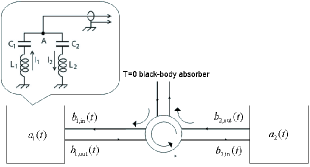
Figure 1: Two identical harmonic oscillators $a_{1}$ and $a_{2}$ coupled to opposite ends of a transmission line. An isolator (round object) placed on the line ensures a unidirectional setup - modes are propagating from oscillator 1 to 2 and from 2 to the termination. A possible implementation of an oscillator as the antisymmetric mode of two lumped circuit resonators is shown in the inset above oscillator 1. This geometry enables good control of the oscillator-line coupling needed for the state transfer. In the symmetric case when $C_{1}=C_{2}$ and $L_{1}=L_{2}$ the antisymmetric mode $I_{1}=I_{2}$ has a voltage node at point $A$ and therefore does not radiate into the transmission line. If the values of the capacitors or inductors are changed to spoil the symmetry, this mode couples into the line.

Finally, we discuss possible realizations of state-transfer setups involving time-dependent switching. In the case of optical cavities, if one is in possession of switches with switching times much faster than the round trip travel time of light within the cavity, complete state transfer could be achieved within one round trip time. In fact, a variety of fast cavity dumping techniques have been developed for pulsed optical systems in which the switching time is considerably faster than the round trip time hook66 ; zitter67 ; bridges69 ; klein70 ; marcus82 ; marchetti01 . The state transfer technique analyzed above is, thus, of most interest in cases where switches fast compared to the round trip time are not available, such as the case of optical cavities with short round trip times. Many cavity dumping techniques hook66 ; marcus82 could be adapted to provide the time-dependent coupling Eq. (14) required for oscillator 1 and a switching time that is fast compared to the ring-down time for oscillator 2.

Since superconducting electronics operating in the microwave frequency range is a contender for quantum computation, how to achieve fast high fidelity quantum state transfer between microwave cavities or lumped circuit LC resonators has become an issue of interest. Cavity dumping techniques have been employed to produce intense microwave pulses from low intensity microwave sources birx78 ; alvarez81 . These techniques often position the output port at a cavity node. Coupling to the outside world is achieved by switching the length of one arm of the cavity so that the output port is no longer positioned at the node. The inset above oscillator 1 in Fig. 1 shows a way in which this idea can be implemented in a resonator consisting of lumped circuit components. If $C_{1}=C_{2}$ and $L_{1}=L_{2}$, the antisymmetric mode of oscillation, for which $I_{1}=I_{2},$ has a voltage node at $A$ and therefore does not radiate into the transmission line. By changing the value of one or more of the inductors or capacitors, the symmetry is spoiled, point $A$ will no longer be a node and this mode will now radiate into the transmission line. The coupling strength is determined by the size of the shift from symmetry. A coupling of the form Eq. (14) can thus be engineered through the use of capacitors and inductors having a controllable time-dependent reactance. Time dependent reactances are generally produced from nonlinear reactors by changing the operating point of the reactance through the application of bias currents or voltages. Examples of a nonlinear reactance that could be used for such an application are Josephson junctions which function as nonlinear inductors, and varactor diodes which function as nonlinear capacitors.

To summarize, we have shown that a transfer of an arbitrary quantum state between two identical harmonic oscillators (optical resonators, electronic oscillators, etc) coupled to distant ends of a transmission line can be achieved with a state-independent fidelity that approaches unity exponentially fast in the coupling switching-time.

K. J. thanks P. Rabl for helpful discussions. This work was supported by the Austrian Academy of Sciences, Austrian Science Fund and the EuroSQIP network.

References

• (1) J. I. Cirac, P. Zoller, H. J. Kimble, and H. Mabuchi, Phys. Rev. Lett. 78, 3221 (1997).
• (2) T. Pellizzari, Phys. Rev. Lett. 79, 5242 (1997).
• (3) S. Bose, Phys. Rev. Lett. 91, 207901 (2003).
• (4) A. Lyakhov and C. Bruder, New J. Phys. 7, 181 (2005).
• (5) M.-H. Yung, quant-ph/0603179
• (6) S. Paganelli, F. de Pasquale and G. L. Giorgi, Phys. Rev. A 74, 012316 (2006).
• (7) M.-H. Yung and S. Bose, Phys. Rev. A 71, 032310 (2005).
• (8) Continuous variable teleportation Kimble12 , in its single-mode form, aims at a transfer of a harmonic oscillator state. Its analysis (see e.g. Ref. MIT ) should thus be applicable to infinite-dimensional Hilbert spaces. However we note that teleportation differs from the state-transfer considered here by the use of a classical information channel.
• (9) S. L. Braunstein and H. J. Kimble, Phys. Rev. Lett. 80, 869 (1998); A. Furusawa et al., Science 282, 706 (1998).
• (10) M. Razavi and J. H. Shapiro, Phys. Rev. A, 73, 042303 (2006).
• (11) B. Yurke and J. S. Denker, Phys. Rev. A 29, 1419 (1984).
• (12) D. F. Walls and G. J. Milburn, Quantum Optics (Springer, New York, 1994).
• (13) See e.g., Eq. (9.60), p. 409, Sec. 9.2.2 in M. A. Nielsen and I. L. Chuang, Quantum Computation and Quantum Information (Cambridge University Press, 2000).
• (14) W. R. Hook, R. H. Dishington, and R. P. Hilberg, Appl. Phys. Lett. 9, 125 (1966).
• (15) R. N. Zitter, W. H. Steier, and R. Rosenberg, IEEE J. Quantum Electronics QE-3, 614 (1967).
• (16) T. J. Bridges and P. K. Cheo, Appl. Phys. Lett. 14, 262 (1969).
• (17) M. B. Klein and D. Maydan, Appl. Phys. Lett. 16, 509 (1970).
• (18) S. Marcus, J. Appl. Phys. 53, 6029 (1982).
• (19) S. Marchetti, M. Martinelli, R. Simili, M. Giorgi, and R. Fantoni, Appl. Phys. B 72, 927 (2001).
• (20) D. Birx, G. J. Dick, W. A. Little, J. E. Mercereau, and D. J. Scalapino, Appl. Phys. Lett. 32, 68 (1978).
• (21) R. A. Alvarez et al., IEEE Trans. Mag. MAG-17, 935 (1981).