Local control of remote entanglement

Abstract

We address the problem of the generation of entanglement. We focus on the control of entanglement shared by two non-interacting parties $A$ and $C$ via interaction with a third party $B$. We show that, for certain physical models, it is possible to have an asymptotically complete control of the entanglement shared by $A$ and $C$ by changing parameters of the Hamiltonian local at site $B$. We present an example where different models (propositions) of physical situation, that lead to different descriptions of the system $B$, result into different amount entanglement produced. In the end we discuss limits of the procedure.

I Introduction

Quantum mechanics admits correlations of a very specific type (entanglement) but the task to create such correlations between several systems need not have a solution under given conditions. A natural way how to correlate two systems is to use mutual (direct) interaction between the two systems. Such approach is unusable where the interaction is weak, the two systems are too far from each other, or simply they do not interact at all. However, even in the extreme case of non-interacting parties there is a possibility to correlate them. Here we basically have two options: First, to perform a joint measurement on the two systems, and second, to use another (ancillary) system. As the first option requires another system, the measurement apparatus, as well, we focus on the second approach where an additional system is used.

If we look at the problem from the operational point of view we can solve the problem in the following way. Let us suppose that we want to create an EPR pair shared by two parties denoted as $A$ and $C$. We denote the additional party used to achieve the goal as $B$. First $B$ creates an EPR pair with party $A$ and a second EPR pair with party $C$. It means that the system $B$ is composed of two qubits. Then by performing two-qubit (Bell) measurement on the two qubits at site $B$ we actually create an EPR pair shared by $A$ and $C$ irrespectively of the outcome of the Bell measurement. The protocol outlined is the “entanglement swapping” protocol proposed by M. Zukowski et. al. Zukowski93 and generalized by S. Bose et. al. Bose98 . The first experimental realization of the protocol was done by J. W. Pan et.al. Pan98 .

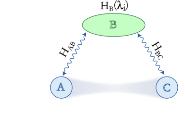
Figure 1: Illustration of the physical situation.

In the entanglement swapping protocol instead of creating entanglement shared by $A$ and $C$ directly we create two maximally entangled pairs one shared by $A$ and $B$ and the second shared by $B$ and $C$. These entangled pairs can be produced using interaction or joint measurement as we have discussed at the beginning. So the entanglement is created in the same way as before and only additional tools are used to transfer this entanglement into correlations between $A$ and $C$.

In order not to use the same approach and explore different ways of creating the entanglement we modify the setup as follows. The two systems $A$ and $C$ interact with the system $B$ and the interaction is described by the Hamiltonians $H_{AB}$ and $H_{BC}$. These Hamiltonians also include the local terms $H_{A}$, and $H_{C}$. Let us remind that the systems $A$ and $C$ do not interact mutually and so the Hamiltonian $H_{AC}$ is zero. In addition, to control the entanglement produced between $A$ and $C$ we use the control of the system $B$ as is illustrated in Fig. 1.

In such scenario we cannot assume that it is possible to create EPR pairs between $A$ and $B$ and $B$ and $C$. The result strongly depends on the choice of the Hamiltonians and if for example the mutual interaction is absent (the local parts can be present though) no entanglement can be produced. In this spirit it is an interesting question under which conditions it is possible to create quantum correlations between $A$ and $C$. It has recently been shown that for a large class of Hamiltonians if we monitor (measure) the system $B$ continuously Zhang03 or even non-continuously but repeatedly Verstraete04 ; Pachos04 ; Wu04 it is indeed possible.

This result can be understood as follows. Let $t$ be the time of the free evolution of the system from the preparation to the measurement. If we prepare the three-partite system in a particular fully-factorized state, then after time $t$ the state of the system $ABC$ can be written as

$$|\psi(t)\rangle_{ABC}=\sum_{j}\>c_{j}(t)\;|\phi_{j}(t)\rangle_{AC}\>|\omega_{j}(t)\rangle_{B}\;,$$

where $|\phi_{j}(t)\rangle_{AC}$ are vectors of unit length, $c_{j}$ are complex coefficients and the basis $\{|\omega_{j}(t)\rangle\}$ corresponds to the measurement that we perform at time $t$. This basis (or measurement) is chosen so that after performing the measurement and projecting the system onto one of the states $|\phi_{j}(t)\rangle_{AC}\>|\omega_{j}(t)\rangle_{B}$ the corresponding state $|\phi(t)\rangle_{AC}$ of the subsystem $AC$ is entangled.

Though the real protocol is more sophisticated, due to the probabilistic nature of the measurement process, and we need to monitor (measure) the system $B$ many times it explains the main idea and the role of the measurement of the system $B$. It is the measurement that projects out the subsystem $AC$ onto an entangled state and the efficiency of detectors, incompleteness of the measurement itself or complexity of the system $B$ can make the monitoring of the system $B$ difficult. As a consequence the entanglement is produced with a low degree or probability. It is an open question whether it is possible to create entanglement between $A$ and $C$ without monitoring the system $B$. In such case the setup is the same as before (see Fig. 1) but the only control that we have is a local “coherent” control of the system $B$. It means that we are allowed to change the parameters of the Hamiltonian local at site $B$ but we are not allowed to perform measurements. So what we can do is to “drive” the Hamiltonian and the system by changing the free parameters $\{\lambda_{i}\}$ of the whole Hamiltonian $H$ of the three partite system $ABC$

$$H=H_{AB}+H_{BC}+H_{B}(\{\lambda_{i}\})\;,$$ (1)

where $\{\lambda_{i}\}$ are the parameters that correspond to the degrees of freedom that we control locally at site $B$. Now the question is how much entanglement between $A$ and $C$ can be created by tuning the parameters $\lambda_{i}$. The answer depends on the choice of the interaction Hamiltonians $H_{AB}$ and $H_{BC}$ and the local control at site $B$. In the following we discuss this dependence as well as the choice of different $B$’s.

The paper is organized as follows. In the next section we address the case where all three systems $A$, $B$ and $C$ are two dimensional systems, that is qubits. We introduce the most general form of Hamiltonian consistent with the assumptions and demonstrate the method on a particular example. In the third section we consider a more complicated case of the Dicke model, where the role of the systems $A$ and $C$ are played by atoms interacting with an electromagnetic field - the system $B$. Here different approximations of the field are analyzed. In the last section we discuss various strategies as well as limits of the method and summarize our results.

II Qubits

We start with the case where the systems $A$, $B$ and $C$ are represented by two-dimensional Hilbert spaces and called qubits. In such case we can write the Hamiltonian $H_{AB}$ as a sum of direct products of Pauli matrices and the identity operator

$$H_{AB}=\sum_{j,k=0}^{3}h_{AB}^{jk}\;\sigma_{A}^{j}\otimes\sigma_{B}^{k}\otimes\openone_{C}\;,$$ (2)

where $\sigma_{l}^{0}$ is the identity operator $\sigma_{l}^{0}=\openone$ and $\sigma_{l}^{j}$, $j=1,2,3$ is the set of three Pauli matrices for each $l=A,B,C$. It means that $\sigma_{l}^{1}=\sigma_{x}$, $\sigma_{l}^{2}=\sigma_{y}$ and $\sigma_{l}^{3}=\sigma_{z}$. In what follows we drop the subscript on operators labeling the system as the position of an operator in a product uniquely specifies to which system the operator corresponds. Real constants, $h_{AB}^{jk}$, $j,k=0,..3$ define the interaction Hamiltonian $H_{AB}$. In the same way the real coefficients $h_{BC}^{jk}$, $j,k=0,..,3$ uniquely define the Hamiltonian $H_{BC}$

$$H_{BC}=\sum_{j,k=0}^{3}h_{BC}^{jk}\;\openone\otimes\sigma^{j}\otimes\sigma^{k}\;.$$ (3)

By local control on site $B$ we understand that we have a choice in tuning the local Hamiltonian $H_{B}$ and more specifically parameters $h_{B}^{j}$ specifying the Hamiltonian

$$H_{B}=\sum_{j=1}^{3}h_{B}^{j}\;\openone\otimes\sigma^{j}\otimes\openone\;.$$ (4)

Note that in this case we did not include the case $j=0$ as such term only shifts energy levels but it does not essentially change the structure of the spectrum and eigenvectors. It means that the set of parameters $\{\lambda_{i}\}$ we control are identified with the three parameters $h_{B}^{j}$, $j=1,2,3$. To see how it works let us consider the following example.

II.1 Ising Interaction

The Ising interaction between the sites $A$ and $B$ is described by the Hamiltonian ising

$$H_{AB}=J\;\sigma^{3}\otimes\sigma^{3}\otimes\openone\;,$$ (5)

where $J$ is the interaction constant and $\sigma^{3}=\sigma^{z}$ is the Pauli operator. Recalling the notation introduced above we obtain that $h_{AB}^{33}=J$ and all other coefficients $h_{AB}^{jk}$, $j,k\neq 3$ are zero. The interaction between $B$ and $C$ is chosen to be the same as it is the interaction between $A$ and $B$ and the Hamiltonian $H_{BC}$ reads

$$H_{BC}=J\;\openone\otimes\sigma^{3}\otimes\sigma^{3}\;.$$ (6)

The physical situation that could be described by the interaction Hamiltonians is following. Assume that the three systems $A$, $B$ and $C$ are of the same type. In such case also the interaction between $A$ and $B$ or $B$ and $C$ is of the same origin. Subsequently if the three systems are positioned in a line and equally spaced then the interaction between $A$ and $C$ is small, in practice negligible, while the interaction between $A$ and $B$ and the interaction between $B$ and $C$ are described by the same Hamiltonian as it is in our case.

The local Hamiltonians $H_{A}$ and $H_{C}$ for the Ising model are of the form

$$H_{A} = \frac{\Delta}{2}\;\sigma^{1}\otimes\openone\otimes\openone\;,$$ (7)

$$H_{C} = \frac{\Delta}{2}\;\openone\otimes\openone\otimes\sigma^{1}\;,$$ (8)

where $\Delta$ is the energy separation between the upper and lower energy level of the two-level system and $\sigma^{1}=\sigma^{x}$ is the Pauli operator. For spin systems the parameter $\Delta$ is proportional to the magnitude of the external magnetic field that is responsible for the splitting of the two energy levels when the spin is placed in the magnetic field. Similarly, the Hamiltonian $H_{B}$ is given by

$$H_{B}=\frac{\Lambda}{2}\openone\otimes\sigma^{1}\otimes\openone\;,$$ (9)

where $\Lambda$ is the energy separation between the two energy levels of the system $B$. For convenience we rewrite the parameters $\Delta$ and $\Lambda$ as $\Delta\rightarrow\delta\Delta_{0}$ and $\Lambda\rightarrow\lambda\Lambda_{0}$. Here $\Delta_{0}$ and $\Lambda_{0}$ are chosen to be $\Delta_{0}=\Lambda_{0}=J$ and $\lambda$ and $\delta$ are dimensionless. In this notation, the parameter that represents the control that we have over the system $B$ is the parameter $\lambda$. Change in the parameter $\lambda$ corresponds to the change of the strength of the external field at site $B$ which determines the energy separation between the two levels of the system $B$.

In what follows we discuss different choices of local Hamiltonians $H_{A}$ and $H_{C}$ and the Hamiltonian $H_{B}$ corresponding to the local control at site $B$. We start with the case where the local terms $H_{A}$ and $H_{C}$ are zero which means that the parameter $\delta=0$. The full Hamiltonian of the system $H$ is a sum of three terms (5), (6) and (9) and the corresponding eigenspectrum can be calculated analytically (see App. A). Due to all of the eigenvectors are factorized it follows immediately that there is no entanglement between $A$ and $C$ irrespective of the local Hamiltonian $H_{B}$. That is by locally controlling the system $B$ it is not possible to create entanglement shared by $A$ and $C$. Note that the degeneracy of the ground state opens a chance to create a state with the lowest energy such that it is entangled. However, as we can create an eigenstate with the same energy but no entanglement, we will not consider such vector as an entangled ground state.

A similar situation occurs when the local Hamiltonians $H_{A}$ and $H_{C}$ are large (large means dominant compared with the interaction terms) so that the parameter $\delta$ is much larger than $1$, that is $\delta\gg 1$. Large energy separation between two levels of systems $A$ and $C$ causes that both of the systems $A$ and $C$ tend to be in their ground state. It follows that the state of the subsystem $AC$ is close to a product of the two ground states, and hence there is no entanglement between $A$ and $C$. Modifying $H_{B}$ cannot change this as the interaction terms are weak compared with the local Hamiltonians $H_{A}$ and $H_{C}$.

On the other hand when the local terms are comparable to the interaction terms or even better when they are small but non-zero the situation changes significantly. First let us consider the local terms $H_{A}$ and $H_{C}$ to be small (but non-zero) in comparison with the interaction terms. It means that the parameter $\delta$ fulfills the relation $\delta\ll 1$. In such case we can consider the local terms to be a perturbation to the full Hamiltonian and calculate the energy levels using the expansion series. As we have already pointed out for the Ising model without the local terms $H_{A}$ and $H_{B}$ the ground state is degenerate and the two levels with the lowest energy are

$$|g_{1}\rangle = |0\rangle\otimes|\alpha_{1}\rangle\otimes|0\rangle\;,$$

$$|g_{2}\rangle = |1\rangle\otimes|\alpha_{7}\rangle\otimes|1\rangle\;,$$

for more details see App. A. If we include the local terms $H_{A}$ and $H_{C}$ in the full Hamiltonian we remove the degeneracy and the ground state becomes non-degenerate. Calculating the ground state to the first order in the parameter $\delta$ with the help of the expansion to the second order (the first order neither removes the degeneracy nor modifies the spectrum but modifies the form of the two ground states) we obtained the state of the form

$$1/K\;\left\{\;|g_{1}\rangle+|g_{2}\rangle+\delta\;[\;|0\rangle\otimes(c_{1}|\alpha_{3}\rangle+c_{2}|\alpha_{4}\rangle)\otimes|1\rangle\right.$$

$$\left.+|1\rangle\otimes(c_{3}|\alpha_{3}\rangle+c_{4}|\alpha_{4}\rangle)\otimes|0\rangle\;]\;\right\}\;,$$

where the complex constants $c_{j}$, $j\!=\!1,..,4$ depend on $\lambda$, $K$ is a normalization constant and the normalized states $|\alpha_{j}\rangle$ are defined in App. A. For $\delta$ small this vector represents an entangled state and for $\delta\!\rightarrow\!0$ the ground state approaches maximally entangled state. Though not explicitly shown in the last equation change in the parameter $\lambda$ causes change in the state (as not only the constants $c_{j}$ but also the states $|\alpha_{j}\rangle$ depend on $\lambda$) and in turn changes the entanglement shared by $A$ and $C$. On the other hand it should be pointed out that the maximal entanglement can be reached only in the limit $\delta\rightarrow 0$ and in the same limit the gap between the ground state and the first excited state vanishes. It means that if we want to increase the maximal amount of entanglement that can be produced between $A$ and $C$ we have to reduce the gap between the two lowest energy levels. As a result of that the cooling of the system (we want our system to stay in the ground state during the whole evolution) is more problematic. The complete picture for arbitrary values of the parameters $\delta$ and $\lambda$ is shown in Fig. (2).

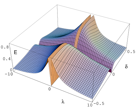
Figure 2: Dependence of the entanglement $E$ shared by $A$ and $C$, expressed as a concurrence (for definition see App. B), on the local control at site $B$, parameter $\lambda$, and for different one-particle Hamiltonians $H_{A}$ and $H_{C}$, parameter $\delta$.

Using simple interaction of Ising type we have shown that it is possible to control (generate) entanglement between essentially distant parties $A$ and $C$. What is important to realize is the fact that the two systems $A$ and $C$ are not allowed to interact and the entanglement is created only through the interaction with the system $B$. In addition, by modifying the site $B$, that is parameters of the local Hamiltonian $H_{B}$, it is possible to control the amount of entanglement shared by $A$ and $C$. In our example the maximal entanglement is actually never reached though we can get arbitrarily close to the maximal possible value. We address this issue in a more detail in the last section.

III Atoms interacting with a single mode electromagnetic field

In our scenario the entanglement between the two parties $A$ and $C$  is generated through the interaction with an auxiliary quantum system at the site $B$ and depends on the choice of the local Hamiltonian $H_{B}$. That is it depends on the physical nature of the system $B$. In the previous section the system $B$ was composed of a single qubit. The situation analyzed in Ref. Bose03 can be considered as a particular case of our scenario where the system $B$ is a collection of spins and the whole system $ABC$ forms a spin chain. It is natural that for different physical systems $B$ we obtain different results. What is not so obvious is the fact that different results are obtained also for different models of a given physical system. Here by different models we have in mind different approximations of the physical situation.

In order to see the problem more clearly we analyze the physical setup composed of two non-interacting atoms placed in a cavity interacting with one mode electromagnetic field. As the two atoms do not interact directly the entanglement can be created only via interaction with the electromagnetic field. Here different approximations lead to different models for the field and one can consider several Hamiltonians.

If we assume a dipole and rotating wave approximation (RWA) and restrict to the case of small interaction between the field and the atomic system, then the system can be described by Dicke Hamiltonian Dicke1954 .

$$H_{1}(\kappa)=\frac{\omega_{A}}{2}\sum_{j}\sigma_{j}^{3}+\omega_{F}a^{\dagger}a+\kappa\sum_{j}(\sigma_{j}^{+}a+\sigma_{j}^{-}a^{\dagger})\;,$$

where the $\sigma_{j}^{+}=\frac{1}{2}(\sigma_{j}^{1}+i\sigma_{j}^{2})$, $\sigma_{j}^{-}=\frac{1}{2}(\sigma_{j}^{1}-i\sigma_{j}^{2})$, the three operators $\sigma^{1}$, $\sigma^{2}$,$\sigma^{3}$ are Pauli operators, $a^{\dagger}$ and $a$ are field creation and annihilation operators, $\omega_{F}$ is the radiation field frequency and $\omega_{A}$ is the atomic transition frequency. The parameter $\kappa$ is proportional to the coupling strength between field and atoms.

The Dicke Hamiltonian is a good starting point in the analysis of the radiation-matter interaction systems, since it can be analytically solved Tavis1967 and describes various (especially collective and cooperative) properties of these systems Wolf .

Nevertheless, if we want to study the system with stronger radiation-atom interaction we must drop the rotating wave-approximation (i.e. it is important to include counter-rotating terms to the Hamiltonian) and in addition an extra quadratic field term, usually neglected, have to be taken into account. When the counter-resonant terms are added the Hamiltonian is of the form:

$$H_{2}(\kappa) = \frac{\omega_{A}}{2}\sum_{j}\sigma_{j}^{3}+\omega_{F}a^{\dagger}a+$$

$$+ \kappa\sum_{j}(\sigma_{j}^{+}a+\sigma_{j}^{-}a^{\dagger}+\sigma_{j}^{+}a^{\dagger}+\sigma_{j}^{-}a)\;,$$

and when in addition the quadratic field term is included the Hamiltonian reads(for more details see Ref. ??):

$$H_{3}(\kappa,\lambda) = \frac{\omega_{A}}{2}\sum_{j}\sigma_{j}^{3}+\omega_{F}a^{\dagger}a+$$

$$+ \kappa\sum_{j}(\sigma_{j}^{+}a+\sigma_{j}^{-}a^{\dagger}+\sigma_{j}^{+}a^{\dagger}+\sigma_{j}^{-}a)$$

$$+ \lambda(a+a^{\dagger})^{2}.$$

In both of the Hamiltonians $H_{2}$ and $H_{3}$ the parameter $\kappa$ denotes the coupling between field and matter and the parameter $\lambda$ that appears in $H_{3}$ is not a free parameter but it is proportional to $\kappa^{2}$ (for more details see Ref. ??).

The quadratic term in the Hamiltonian (III) is not only necessary for the cases of stronger interactions from the physical point of view, but it is also useful for the mathematical analysis, how an extra non-interaction term included into the Hamiltonian influences the properties of the system.

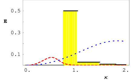
Figure 3: Concurrence $E$ of the two atoms in the cavity as a function of the coupling $\kappa$ for three different types of Hamiltonians $H_{1}$ (black solid line), $H_{2}$ (red dashed line) and $H_{3}$ (blue dashed line). The behavior of the bi-partite entanglement in the two atom system is clearly different for the three Hamiltonians. The amount of quantum correlation in the system depends on and thus can be controlled by the strength of the interaction. It is apparent from the figure that for the case of Hamiltonian $H_{3}$ the concurrence persists also in the cases of stronger interactions and in average it has larger values compared with cases of $H_{1}$ and $H_{2}$.

In what follows, we will study how the change of the parameters $\kappa$ and $\lambda$ influences the entanglement between individual two particles of the atomic system. More specifically, we will study bi-partite atomic entanglement in the ground state of the systems described by the Hamiltonians $H_{1}$, $H_{2}$ and $H_{3}$. Finally, we will compare the results. Since atoms are described as two-level quantum systems, we will use the concurrence of a reduced bipartite atomic system as an entanglement measure.

Firstly, we focus on how the quadratic field term in Hamiltonian $H_{3}$ influences the bi-partite entanglement, comparing to the Hamiltonians without this term ($H_{1}$ and $H_{2}$). From all tree Hamiltonians, only Hamiltonian $H_{1}$ can be diagonalized analytically Tavis1967 ; Buzek2005 , therefore we have done an numeric analysis and we will discuss the results on figures. It is apparent from the Fig. 3 that the bi-partite atomic entanglement is significantly different in the three cases studied. The main property of the concurrence for the Hamiltonians $H_{1}$ and $H_{2}$ (i.e. without non-interacting term) is that their values drop to $E=0$ very quickly. On the other hand the presence of the quadratic non-interacting field term in $H_{3}$ ensures that the quantum correlations persist also in the cases of strong interaction between field and atomic system. In addition, two atoms are (in average) more entangled compared with the previous cases as it can be seen from the Fig. 3.

Further, let us separately study how the bi-partite entanglement in the atomic system is controlled by the strength of the interaction (parameter $\kappa$) and the size of the quadratic term (parameter $\lambda$) in the case of the complete Hamiltonian $H_{3}$. We note that this is rather mathematical approach since $\lambda$ is not independent from the coupling ($\lambda\sim\kappa^{2}$) but it can illuminate how the non-interacting field term can have an influence on the entanglement between individual atoms - even for fixed coupling $\kappa$. Again, all calculations were made numerically and our results will be discussed with the help of the Fig. 4.

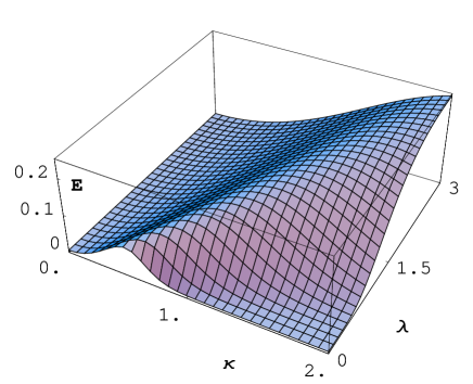
Figure 4: Bipartite entanglement $E$ (concurrence) between the two atoms as a function of the coupling $\kappa$ and the parameter $\tilde{\lambda}$. It is apparent from the figure that we can control (increase) the bipartite entanglement by increasing the system interaction $\kappa$ or by increasing the quadratic term independently (the parameter $\tilde{\lambda}$).

As it is illustrated in the figure, by the change in the parameters in the quadratic field term ($\lambda\rightarrow\tilde{\lambda}\lambda$ ) we can control the strength of the bi-partite quantum correlations in the atomic system. These get stronger as the interaction between field and atomic system increases (increasing $\kappa$) or when we independently increase the quadratic term (increasing $\tilde{\lambda}$).

IV General case

In this section we address the limits of the studied scheme and for that we introduce the following theorem.

Theorem: Consider Hamiltonian (1) that is symmetric under exchange of the labels (systems) $A$ and $C$. Further let $|\psi\rangle_{ABC}$ be an eigenstate of the Hamiltonian $H$ such that it is of the form $|\psi\rangle_{ABC}=|\omega\rangle_{AC}\otimes|\beta\rangle_{B}$.

If the energy level corresponding to the state $|\psi\rangle_{ABC}$ is non-degenerate then the state $|\psi\rangle_{ABC}$ is fully factorized so that $|\omega\rangle_{AC}=|\alpha\rangle_{A}\otimes|\gamma\rangle_{C}$.

Proof: First we rewrite the state $|\psi\rangle_{ABC}$ so that we decompose the state $|\omega\rangle_{AC}$ using the Schmidt basis

$$|\psi\rangle_{ABC}=\sum_{j}\sqrt{\lambda}_{j}|j\rangle_{A}\otimes|\beta\rangle_{B}\otimes|j\rangle_{C}\;,$$ (11)

where $\lambda_{j}$ are eigenvalues of the density operator corresponding to the state $\rho_{A}={\rm Tr}_{C}(|\omega\rangle\langle\omega|)$ and $\{|j\rangle_{A}\}$ and $\{|j\rangle_{C}\}$ is the Schmidt basis of the system $A$ and $C$ respectively. Applying Hamiltonian (1) to the state (11) we obtain the expression

$$H|\psi\rangle_{ABC}=\sum_{j}\sqrt{\lambda}_{j}[|w_{j}\rangle_{AB}\otimes|j\rangle_{C}+|j\rangle_{A}\otimes|w_{j}\rangle_{BC}]\;,$$

where $|w_{j}\rangle_{AB}=(H_{AB}+H_{B}/2)|j\rangle_{A}\otimes|\beta\rangle_{B}$, $|w_{j}\rangle_{BC}=(H_{BC}+H_{B}/2)|\beta\rangle_{B}\otimes|j\rangle_{C}$. The action of the Hamiltonian $H$ was divided into two parts: the interaction between $A$ and $B$ and the interaction between $B$ and $C$. In order to preserve symmetry under the exchange of $A$ and $C$ the term corresponding to the local control at site $B$ was divided into two equal parts. One of them was added to $H_{AB}$ and the other to $H_{BC}$. Notice that the states $w_{j}$ need to be neither normalized nor mutually orthogonal. For the state $|\psi\rangle_{ABC}$ to be an eigenstate of the Hamiltonian the reduced operator of the system $B$ has to be proportional to the projection $|\beta\rangle_{B}\langle\beta|$ (in the propositions of the theorem we assume a particular form of the state $|\psi\rangle_{ABC}$). It follows that the action of the Hamiltonian is restricted  and

$$(H_{AB}+H_{B}/2)|j\rangle_{A}\otimes|\beta\rangle_{B} = |v_{j}\rangle_{A}\otimes|\beta\rangle_{B}\;,$$

$$(H_{BC}+H_{B}/2)|\beta\rangle_{B}\otimes|j\rangle_{C} = |\beta\rangle_{B}\otimes|v_{j}\rangle_{C}\;,$$

where the vectors $|v_{j}\rangle$ are unnormalized in general. In addition, the state $H|\psi\rangle_{ABC}$ has to be orthogonal to the state of the form $|j\rangle_{A}\otimes|\beta\rangle_{B}\otimes|k\rangle_{C}$ where $k\neq j$. It follows that $\langle k|v_{j}\rangle=0$ for $k\neq j$ and the action of $H_{AB}+H_{B}/2$ (correspondingly $H_{BC}+H_{B}/2$) is of the form

$$(H_{AB}+H_{B}/2)|j\rangle_{A}\otimes|\beta\rangle_{B}\otimes|j\rangle_{C}=c_{j}|j\rangle_{A}\otimes|\beta\rangle_{B}\otimes|j\rangle_{C}\;.$$

Finally, if the sum over $j$ in (11) includes only a single term then the state $|\psi\rangle_{ABC}$ is fully factorized. On the other hand if the sum includes two and more terms then the constants $c_{j}$ for that terms have to be equal (independent of $j$). However in such case the energy level corresponding to that state is degenerate. It follows from the fact that using the expressions for $H_{AB}$ and $H_{BC}$ derived above it is possible to show that the states of the form $\sum_{j}c_{j}|j\rangle_{A}\otimes|\beta\rangle_{B}\otimes|j\rangle_{C}$, where $c_{j}$ are arbitrary complex numbers up to normalization, have the same energy.

The Theorem has important implications concerning the creation of entanglement between $A$ and $C$. It follows from the theorem that using the method it is not possible to create a maximally entangled state shared by $A$ and $C$. More specifically, if the ground state of the system $ABC$ is such that the reduced state of $AC$ is a maximally entangled state then we know from the theorem that the ground state is degenerate and it is possible to create a non-entangled state with the same energy so we should not consider such ground state as entangled. On the other hand we can be arbitrarily close to a maximally entangled state and this was demonstrated in the Sec. II.

Further, applying the theorem more generally we can state that in this scenario it is not possible to create any pure entangled state shared by $A$ and $C$. It means that by modifying the local parameters at site $B$ and not considering measurements the ground state of the system $ABC$ is such that the reduced state $\rho_{AC}$ of the systems $A$ and $C$ can be entangled only if it is mixed.

To summarize, we have analyzed a particular scenario of the generation of entangled where the entanglement is produced via interaction with additional system and no measurements are considered. We have shown that under the symmetry condition the maximal entanglement can be reached only asymptotically and no pure entangled state can be produced. Moreover, we have shown that different assumptions about the additional physical system $B$ result into situations where different amount of entanglement is produced.

Acknowledgement

This work was supported in part by the European Union projects INTAS-04-77-7289, CONQUEST and QAP, by the Slovak Academy of Sciences via the project CE-PI/2/2005, by the project APVT-99-012304.

Appendix A Ising model

In this appendix we present the eigenvectors and corresponding eigenvalues of the Ising Hamiltonian (5) without the local terms at sites $A$ and $B$ but with the most general local term at site $B$. The Hamiltonian $H$ with the Ising type interaction between sites $A$ and $B$ and sites $B$ and $C$ together with the most general local term corresponding to the site $B$ is of the form

$$H = \sigma^{3}\otimes\sigma^{3}\otimes\openone+\openone\otimes\sigma^{3}\otimes\sigma^{3}$$

$$+\openone\otimes(\sum_{j}h_{B}^{j}\sigma^{j})\otimes\openone\;.$$

The eigenvectors of the Hamiltonian $H$ with the corresponding eigenvalues are listed below

$$\begin{array}[]{lll}e_{1,2}=|0\rangle\otimes|\alpha_{1,2}\rangle\otimes|0\rangle,&E_{1,2}=\pm\sqrt{\sum_{j}(h_{B}^{j}+v^{j})^{2}}\;,\\ e_{3,4}=|1\rangle\otimes|\alpha_{3,4}\rangle\otimes|0\rangle,&E_{3,4}=\pm\sqrt{\sum_{j}(h_{B}^{j})^{2}}\;,\\ e_{5,6}=|0\rangle\otimes|\alpha_{5,6}\rangle\otimes|1\rangle,&E_{5,6}=\pm\sqrt{\sum_{j}(h_{B}^{j})^{2}}\;,\\ e_{7,8}=|1\rangle\otimes|\alpha_{7,8}\rangle\otimes|1\rangle,&E_{7,8}=\pm\sqrt{\sum_{j}(h_{B}^{j}-v^{j})^{2}}\;,\\ \end{array}$$

where $v^{j}=(0,0,2)$, and the vectors $|\alpha_{j}\rangle$, $j=1,2$ are two eigenvectors of the operator $h_{B}^{j}\sigma^{j}+2\sigma^{3}$, the vectors $|\alpha_{j}\rangle=|\alpha_{j+2}\rangle$, $j=3,4$ are eigenvectors of the operator $\sum_{j}h_{B}^{j}\sigma^{j}$ and the vectors $|\alpha_{j}\rangle$, $j=7,8$ are eigenvectors of the operator $\sum_{j}h_{B}^{j}\sigma^{j}-2\sigma^{3}$.

Appendix B Concurrence

In this appendix we recall the definition of the concurrence Wootters97 which is a measure of bipartite entanglement shared by two qubits (quantum systems associated to two-dimensional Hilbert spaces). Let $\rho_{AB}$ be a bipartite state (density matrix) of a two-qubit system. Further, denote as $\lambda_{i}$, $i=1,2,3,4$ the eigenvalues of the matrix $\rho_{AB}\;\sigma^{2}\otimes\sigma^{2}\rho_{AB}^{*}\;\sigma^{2}\otimes\sigma^{2}$ listed in a non-decreasing order. Here $\rho_{AB}^{*}$ means complex conjugation of the matrix $\rho_{AB}$ and $\sigma^{2}$ is the Pauli operator corresponding to the measurement of the spin along the $y$ axis. Then the concurrence $E$ is defined as

$$E(\rho_{AB})\equiv{\rm Max}\{0,\sqrt{\lambda_{1}}\!-\!\sqrt{\lambda_{2}}\!-\!\sqrt{\lambda_{3}}\!-\!\sqrt{\lambda_{4}}\}.$$ (13)

References

- (1) M. Zukowski, A. Zeilinger, M. A. Horne, and A. K. Ekert: “Event-ready-detectors” Bell experiment via entanglement swapping Phys. Rev. Lett. 71, p. 4287 (1993)
- (2) S. Bose, V. Vedral, and P. L. Knight: Multiparticle generalization of entanglement swapping Phys. Rev. A 57, p. 822 (1998)
- (3) J. W. Pan, D. Bouwmeester, H. Wienfurter, and A. Zeilinger: Experimental Entanglement Swapping: Entangling photons that never interacted Phys. Rev. Lett. 80, p. 3891, (1998)
- (4) D. Kielpinski, C. R. Monroe, and D. J. Wineland: Architecture for a large-scale ion-trap quantum computer Nature 417, 709 (2002).
- (5) J. Zhang, J. Vala, S. Sastry, and K. B. Whaley Geometric theory of nonlocal two-qubit operations Phys. Rev. A 67, 042313 (2003).
- (6) F. Verstaete, M. A. Martin-Delgado, and J. J. Cirac: Diverging entanglement length in gapped quantum spin systems Phys. Rev. Lett. 92, 087201 (2004)
- (7) J. K. Pachos and M. B. Plenio: Three-spin interactions in optical lattices and criticality in cluster hamiltonians Phys. Rev. Lett. 93, 056402 (2004)
- (8) L.-A. Wu, D. A. Lidar, and S. Schneider: Long-range entanglement generation via frequent measurements Phys. Rev. A 70, 032322 (2004).
- (9) see for instance S. Sachdev: Quantum Phase Transitions (Cambridge University Press, 1999), Chapter 1.
- (10) S. Bose: Quantum communication through an unmodulated spin chain Phys. Rev. Lett. 91, 207901 (2003)
- (11) W. K. Wootters and S. Hill: Entanglement of formation of an arbitrary state of two qubits Phys. Rev. Lett. 78, p. 5022, (1997)
- (12) R.H. Dicke: Coherence in spontaneuos radiation processes Phys. Rev. 93, 99 (1954).
- (13) M. Tavis and F.W. Cummings: Exact Solution for an N-Molecule-Radiation-Field Hamiltonian Phys. Rev. 170, 379.
- (14) L. Mandel and E. Wolf: Optical coherence and quantum optics (Cambridge University Press, 1995), Chapter 16.
- (15) V. Bužek, M. Orszag, and M. Roško: Instability and entanglement of the ground state of the Dicke model Phys. Rev. Lett. 94, 163601(2005).