Laser-noise-induced correlations and anti-correlations in Electromagnetically Induced Transparency

Abstract

High degrees of intensity correlation between two independent lasers were observed after propagation through a rubidium vapor cell in which they generate Electromagnetically Induced Transparency (EIT). As the optical field intensities are increased, the correlation changes sign (becoming anti-correlation). The experiment was performed in a room temperature rubidium cell, using two diode lasers tuned to the ⁸⁵Rb $D_{2}$ line ($\lambda=780$nm). The cross-correlation spectral function for the pump and probe fields is numerically obtained by modeling the temporal dynamics of both field phases as diffusing processes. We explored the dependence of the atomic response on the atom-field Rabi frequencies, optical detuning and Doppler width. The results show that resonant phase-noise to amplitude-noise conversion is at the origin of the observed signal and the change in sign for the correlation coefficient can be explained as a consequence of the competition between EIT and Raman resonance processes.

1 Introduction

Electromagnetically Induced Transparency (EIT) has received great attention in recent years in connection to several interesting phenomena, such as light storage and slow light propagationHau99 ; Liu01 ; Bajcsy03 . The strong interaction between light and material media in this situation has been the source of inspiration for various proposals of applications of EIT to the quantum manipulation of information and to transfer coherence from light to an atomic mediumLiu01 ; Wal03 ; Beausoleil04 .

The strong interaction between pump and probe fields in EIT can lead to significant changes in the noise spectra of two independent lasers after propagation in an atomic vapor, resulting in correlation between the fields, as was first observed in Ref. Garrido-Alzar03 . A recent paper Huss04 reported an experimental investigation of the dependence of the phase correlation between both fields generating EIT as a function of the optical depth and transparency frequency window. The phase modulation (PM) introduced on the pump field could be read in the probe field signal after interaction with the atoms, for a Raman detuning within the transparency window. Nevertheless, no distinction between positive and negative correlation was reported in that paper. The possibility of negative correlations for large Raman detunings is discussed in Ref. Barberis-Blostein04 , which presents theoretical calculations for the correlation between the pump and probe fields in EIT configuration caused by the atomic dipole fluctuations.

In this paper, we report new measurements in which this kind of correlation originates from two independent lasers. Both fields excite an atomic sample forming a $\Lambda$ system, resulting in a EIT situation. We define a normalized correlation coefficient $C$, bounded by -1 and +1, and report measurements of $C$ as a function of intensity and analysis frequency. As the laser intensities are increased, intensity correlations become anti-correlations. Correlations and anti-correlations as big as 0.65 and -0.65, respectively, were observed. The results can be explained in terms of the conversion of Phase-Noise into Amplitude-Noise (PN-to-AN) as the lasers interact resonantly with the atomic medium. The passage from correlation to anti-correlation can be seen as a consequence of the passage from EIT to a Raman resonance, both present in a 3-level atom in the $\Lambda$ configuration.

PN-to-AN conversion in atomic vapors has been studied since 1991, when its application to high-resolution spectroscopy was first suggested by Yabuzaki et al.Yabuzaki91 . This conversion relies on the characteristics of diode lasers, which exhibit excess phase noise for usual experimental conditionsPetermann91 ; Zhang95 while the amplitude is generally very stable. This excess phase noise generates amplitude noise of the polarization induced in the atomic mediumYabuzaki91 ; Walser94a and the intensity fluctuation spectrum of the transmitted light is strongly dependent on the laser linewidthCamparo99 . Since the fields detected after the medium are given by the input fields plus the excited polarizations, they end up acquiring excess noise in the amplitude quadrature. The spectral noise components that match atomic resonance frequencies present larger amplitude oscillations. In this way, it is possible to acquire information about the medium from the power spectrum of light after the sampleYabuzaki91 ; McIntyre93 ; Bahoura01 . The influence of laser fluctuations on the atomic polarization has been widely studied for two-level systemsWalser94b ; Anderson90a ; Anderson90b and many models have been proposed for treating the field phase fluctuationRitsch90 ; Walser94a . The phase diffusing model has received more attention owing to its proximity to the diode lasers extensively used in laboratories. In a recent experimentMartinelli04 , we performed measurements of intensity noise spectra between the $\sigma^{+}$ and $\sigma^{-}$ components of a single, linearly polarized, exciting field in a Rb atomic sample, as a function of the magnetic field in a Hanle/EIT configuration. We observed correlations as well as anti-correlations between the different polarization components, depending on the detuning, controlled by the magnetic field. A similar experiment was performed by Sautenkov et al.Sautenkov05 , using two initially phase-correlated beams in time domain, who also explained it in terms of PN-to-AN conversionAriunbold05 . In Ref. Camparo05 PN-to-AN conversion has also been identified as a source of frequency instabilities in Rb atomic clocks, and was eliminated with a buffer gas cell that broadens the resonances through collisions.

In the present work, the emphasis is on the PN-to-AN conversion as a source of correlation between initially independent macroscopic fields. The paper is organized as follows: in section 2 we describe our experimental setup and in section 3 we present a theoretical model that includes two phase diffusing fields interacting with an atomic system. In section 4 we present our results, beginning with the experimental correlation spectra as a function of the analysis frequency and optical intensity. Then, in section 4b, we present the numerical results and discussion. As described below, although it is possible to extract the basic aspects of the phenomena by modeling the atomic system as 3-level atoms at rest, agreement with experimental data is considerably improved by integrating over the atoms’ different velocity classes and including all the relevant excited atomic levels. We also found that the optical detuning is essential for explaining the change in sign for the correlation coefficient. For a perfectly resonant $\Lambda$ system, the EIT process is dominant and the fields become correlated but, for an optical detuning of the order of the excited-level decay rate, the Raman process prevails and the fields become anti-correlated.

2 Experimental setup

Our experimental setup is shown in Fig. 1. We employed two external-cavity diode lasers (ECDLs) of 1 MHz linewidth and 15 mW power after optical isolators, tuned to the Rubidium $D_{2}$ line ($\lambda=780$ nm). The two beams had linear orthogonal polarizations and were combined in a polarizing beam splitter (PBS). Their powers were adjusted to have equal intensities at the vapor cell. A small portion of Laser 2 was sent to a saturated absorption setup for fine tuning, and had its frequency locked to the cross-over peak between the $5S_{1/2}(F=3)\rightarrow 5P_{3/2}(F^{\prime}=2)$ and $5S_{1/2}(F=3)\rightarrow 5P_{3/2}(F^{\prime}=4)$ transitions of ⁸⁵Rb. The rejected output of the polarizing beam splitter is used to observe EIT in an auxiliary vapor cell. Laser 1, tuned to the $5S_{1/2}(F=2)\rightarrow 5P_{3/2}(F^{\prime})$ transition, is then locked on the EIT resonance using a Lock-in amplifier (see Fig. 1). In this way, we guarantee that the Raman resonance condition for EIT was always fulfilled. Both lasers were locked only by feedback applied to their external cavity gratings. The laser intensities were controlled by neutral density filters inserted just before the main vapor cell. We also used a 2 mm-diameter diaphragm to spatially filter the laser beams, ensuring a good spatial superposition and a flat, nearly top-hat, intensity profile over the cell.

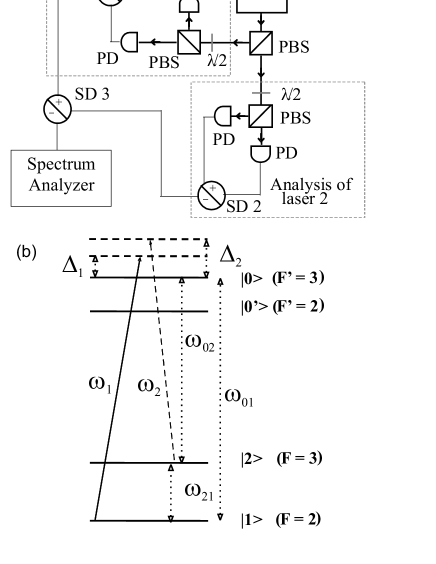
Figure 1: (a) Experimental setup. The saturated absorption setup for laser 2 is not shown. OI: optical isolator; PBS: polarizing beam splitter; PD: photo-detector; NF: neutral filter; $\lambda/2$: half-wave plate.(b) Energy level representation for our atomic model and its correspondence to the relevant Rb hyperfine states. Solid line represents the pump field with frequency $\omega_{1}$; dashed line represents the probe field with frequency $\omega_{2}$.

After the cell, the beams were separated at a second PBS and then analyzed at two independent balanced-detection schemes. Photocurrents were combined in active sum/subtraction circuits (SD), and noise was measured with a Spectrum Analyzer. Effective bandwidth of our detection is limited by the gain of the amplifiers in the range of 2.5 to 14 MHz. Beyond this frequency, electronic noise reduced the resolution of our measurements. We can, therefore, measure the Sum $S_{s}(\omega)$ and Difference $S_{d}(\omega)$ noise spectra, as well as the individual laser noise spectra $S_{11}(\omega)$ and $S_{22}(\omega)$ by blocking a beam on each balanced detection. It is then possible to obtain the normalized correlation coefficient defined by

$$C(\omega)=\frac{S_{12}(\omega)}{\sqrt{S_{11}(\omega)S_{22}(\omega)}}.$$ (1)

The symmetrical cross-correlation spectrum $S_{ij}(\omega)$ between the lasers $i$ and $j$ is defined by

$$S_{ij}(\omega)=\frac{1}{2}\langle\delta I_{i}(\omega)\delta I_{j}(\omega)^{*}+\delta I_{j}(\omega)\delta I_{i}(\omega)^{*}\rangle.$$ (2)

Thus, $S_{12}$ can be obtained from

$$S_{s}=S_{11}+S_{22}+2S_{12}\,,$$ (3a)

$$S_{d}=S_{11}+S_{22}-2S_{12}\,.$$ (3b)

$$S_{12}=\frac{1}{4}(S_{s}-S_{d})$$ (3c)

A summary of all possibilities allowed by our setup is presented in Table  1. If Laser 1 is blocked, one uses the SD2 circuit to calibrate shot noise (with the subtraction position of SD2) or measure the total noise (with the sum position of SD2) of Laser 2. If one blocks the Laser 2, an analogous reasoning is valid for the SD1 circuit. The sum and difference noise spectra expressed in  (3) are obtained with the SD1 and SD2 switches both in the sum position and changing the SD3 switch.

Measurement	Beam blocked	SD1	SD2	SD3
Total noise 1 ($S_{11}$)	Laser 2	$+$	n.i.	n.i.
s.n. of Laser 1	Laser 2	$-$	n.i.	n.i.
Total noise 2 ($S_{22}$)	Laser 1	n.i.	$+$	n.i.
s.n. of Laser 2	Laser 1	n.i.	$-$	n.i.
Sum ($S_{s}$)	none	$+$	$+$	$+$
Diff. ($S_{d}$)	none	$+$	$+$	$-$

Table 1: Summary of the different possibilities of noise measurements. s.n. means shot-noise; n.i. stands for no influence.

3 Theoretical Model

3.1 The phase diffusing field

We developed a model based on Bloch equations. In the $D_{2}$ line of ${}^{85}Rb$ two excited levels (out of 4 levels inside the Doppler broadened curve) can lead to EIT with the hyperfine ground states. Inclusion of a second excited level is important to give a better agreement with the experimental curves. The atom is excited by two classical fields that will be considered as having constant amplitudes and independent stochastic phase fluctuations. Our model is an adaptation of the model of Ref.Walser94a for a three-level atom. The four levels are represented in Fig. 1, where we made a correspondence of the hypothetical quantum states to the realistic levels of ⁸⁵Rb. The two ground states $|1\rangle$ and $|2\rangle$ correspond to ⁸⁵Rb $5S_{1/2}$($F=2$) and ($F=3$), and the excited states $|0^{\prime}\rangle$ and $|0\rangle$ stand for the $5P_{3/2}(F^{\prime}=2)$ and $(F^{\prime}=3)$ levels, respectively. We notice that these levels form two $\Lambda$ systems for atoms of two velocity classes differing by $kv\simeq 64$ MHz, and the EIT resonance in the room temperature vapor is built up from nearly equal contributions of both these $\Lambda$ systems. Although all these four levels are important for a good agreement with experimental data, for the sake of simplicity we present an outline of calculations for a three level system (excluding the excited $|0^{\prime}\rangle$ level). The 3-level system can already reproduce many of the experimental aspects associated to the EIT resonance Garrido-Alzar03 ; Martinelli04 . Further inclusion of the fourth level is straightforward. In the following sections we will present numerical results for both cases.

The laser fields are given by

$$\mathbf{E}_{i}(t)={\cal E}_{i}\exp{[i(\omega_{i}t+\phi_{i})]}\mathbf{e}_{i},$$ (4)

where $i=1,2$ is a label to designate lasers 1 and 2, respectively. $\mathcal{E}_{i}$ is the laser’s complex amplitude, $\omega_{i}$ its frequency and $\mathbf{e}_{i}$ is a unit vector designating the field’s polarization. The time evolutions of the phases $\phi_{1}(t)$ and $\phi_{2}(t)$ are described by two independent, uncorrelated Wiener processesGardiner83 . This corresponds to model the lasers as phase-diffusing fields, with Lorentzian lineshapesWalser94a . Phase fluctuations satisfy the relations

$$\langle\mathrm{d}\phi_{j}\rangle=0,\qquad\langle\mathrm{d}\phi_{j}\mathrm{d}\phi_{k}\rangle=2\sqrt{b_{j}b_{k}}\delta_{jk}\mathrm{d}t$$ (5)

where $2b_{j}$ corresponds to the spectral width of laser $j$ and $\langle\cdots\rangle$ denotes stochastic average that is taken over a sufficiently long time. The $\delta_{jk}$ function accounts for the initial independence of the two lasers in our experiment, so they have a zero degree of correlation.

For an optically thin sample, the output field can be written as

$$\mathbf{E}_{out}(t)=\mathbf{E}_{1}(t)+\mathbf{E}_{2}(t)+i\frac{\beta}{2c\epsilon_{0}}\mathbf{P}(t),$$ (6)

where $\beta$ is a real constant depending on the atomic density and length of the sample, and $\mathbf{P}$ is the complex polarization excited in the medium given by

$$\mathbf{P}(t) =\int_{-\infty}^{\infty}\mathrm{d}\omega_{01}g(\omega_{01})\mathbf{p}_{1}(t,\omega_{01})\exp{[i(\omega_{1}t+\phi_{1})]}+$$

$$\int_{-\infty}^{\infty}\mathrm{d}\omega_{02}g(\omega_{02})\mathbf{p}_{2}(t,\omega_{02})\exp{[i(\omega_{2}t+\phi_{2})]}\,.$$ (7)

In this expression, the inhomogeneous Doppler broadening is given by $g(\omega_{0i})$, for atoms with resonance frequencies $\omega_{0i}$ in the laboratory reference frame. $\mathbf{p}_{1}(t,\omega_{01})$ and $\mathbf{p}_{2}(t,\omega_{02})$ are the slowly-varying atomic coherences excited by fields 1 and 2, respectively.

The detected intensities of fields 1 and 2 are given by $I_{q}(t)=2\,c\,\epsilon_{0}\,|\mathbf{E}_{out}(t)\cdot\mathbf{e}_{q}(t)|^{2}$, where $q=1,2$. All power spectra can be obtained from the expression

$$S_{qq^{\prime}}(\omega)=\int_{-\infty}^{\infty}[\langle I_{q}(t+\tau)I_{q^{\prime}}(t)\rangle- \langle I_{q}(t+\tau)\rangle\langle I_{q^{\prime}}(t)\rangle]$$

$$\times\exp{(i\omega\tau)}\mathrm{d}\tau,$$ (8)

and we recall that the sum and difference spectra are given by Eqs. (3). If we discard terms of second order in $\beta$ and terms independent of $\tau$, and use Eqs. (6) to (8), we can write

$$S_{qq^{\prime}}(\omega)= \beta^{2}{\cal E}_{q}{\cal E}_{q^{\prime}}\int_{-\infty}^{\infty}\mathrm{d}\omega_{0q}\int_{-\infty}^{\infty}\mathrm{d}\omega_{0q^{\prime}}^{\prime}g_{q}(\omega_{0q})g_{q^{\prime}}(\omega_{0q^{\prime}})$$

$$\{-\int_{-\infty}^{\infty}\mathrm{d}\tau\exp{i\omega\tau}[\langle p_{q}(t+\tau,\omega_{0q})p_{q^{\prime}}(t,\omega^{\prime}_{0q^{\prime}})\rangle$$

$$-\langle p_{q}(t,\omega_{0q})\rangle\langle p_{q^{\prime}}(t,\omega^{\prime}_{0q^{\prime}})\rangle]+$$

$$\int_{-\infty}^{\infty}\mathrm{d}\tau\exp{i\omega\tau}[\langle p_{q}(t+\tau,\omega_{0q})p^{*}_{q^{\prime}}(t,\omega^{\prime}_{0q^{\prime}})\rangle$$

$$-\langle p_{q}(t,\omega_{0q})\rangle\langle p^{*}_{q^{\prime}}(t,\omega^{\prime}_{0q^{\prime}})\rangle]+cc\},$$ (9)

where we can see that the power spectra are obtained from the covariance matrix of the detected intensities, which are then ultimately related to the covariance matrix for the atomic variables $p_{1}=|\mathbf{p_{1}}|$ and $p_{2}=|\mathbf{p_{2}}|$. We now present an outline for the calculation of the atomic covariance matrix for the case of a three level atom excited by two phase-diffusing fields. More details can be found in Ref. Walser94a , especially in its Appendix B.

3.2 Atomic polarization spectra

The total Hamiltonian can be written as

$$H(t)=H_{0}+V(t),$$ (10)

where $H_{0}=\hbar\omega_{01}|0\rangle\langle 0|+\hbar\omega_{21}|2\rangle\langle 2|$ is the free-atom Hamiltonian and

$$V(t)= -\hbar\Omega_{1}\exp{[i(\omega_{1}t+\phi_{1})]}|1\rangle\langle 0|$$

$$-\hbar\Omega_{2}\exp{i(\omega_{2}t+\phi_{2})}|2\rangle\langle 0|,$$ (11)

is the interaction Hamiltonian, with the corresponding Rabi frequencies for both coupling fields given by $\Omega_{j}$. Since no detailed Zeeman structure is considered, we took both Rabi frequencies as real. We now follow straightforward steps to write the Bloch equations, in the Liouville form, from (10) and imposing the Rotating Wave Approximation (RWA), which results in

$$\mathrm{d}y=exp[iN_{1}(\omega_{1}t+\phi_{1})]exp[iN_{2}(\omega_{2}t+\phi_{2})]Ax\mathrm{d}t$$

$$+y_{0}\mathrm{d}t\;.$$ (12)

Here $N_{1}$ and $N_{2}$ are square diagonal matrices with only zeros and ones, $y_{0}$ is a column matrix accounting for the continuous flow of atoms through the laser beam and $A(\Omega_{1},\Omega_{2},\\ \Gamma,\gamma,\Delta_{1},\Delta_{2},\delta_{R})$ is the evolution Bloch matrix, that is function of several physical parameters: $\Gamma$ is the total excited state decay rate, $\gamma$ is a decay rate for the lower states coherence associated to the finite interaction time, $\Delta_{j}=\omega_{j}-\omega_{0j}$ is the optical detuning associated to laser $j$, and $\delta_{R}=\Delta_{1}-\Delta_{2}$ is the Raman detuning. The column matrices containing the rapid and slowly varying elements of the atomic density matrix are $y$ and $x$, respectively. They are related by the transformation

$$x=exp[-iN_{1}(\omega_{1}t+\phi_{1})]exp[-iN_{2}(\omega_{2}t+\phi_{2})]y.$$ (13)

We have special interest in the $x$ matrix, because it contains the slowly varying atomic coherences ($p_{01},p_{02},p_{12}$, and their conjugates). To proceed with the calculations of the stochastic averages one must expand the exponential factors up to second order in the $\mathrm{d}\phi_{j}$’s and take averages using eq.(5), resulting in a differential equation for $\langle x\rangle$

$$\mathrm{d}\langle x\rangle=[-A_{1}\langle x\rangle+y_{0}]\mathrm{d}t$$ (14)

with

$$A_{1}=iN_{1}\omega_{1}+iN_{2}\omega_{2}+b_{1}N_{1}^{2}+b_{2}N_{2}^{2}-A,$$ (15)

whose steady state solution is

$$\langle x\rangle=A_{1}^{-1}y_{0}.$$ (16)

However, products in the form $\langle p_{q}(t+\tau,\omega_{0q})p^{*}_{q^{\prime}}(t,\omega^{\prime}_{0q^{\prime}})\rangle$ and $\langle p_{q}(t+\tau,\omega_{0q})p_{q^{\prime}}(t,\omega^{\prime}_{0q^{\prime}})\rangle$ appear in equation (9). To evaluate these terms it is convenient to first calculate the second order correlation function

$$\langle G(t,t;\omega_{0j},\omega_{0k})\rangle=\langle x(t,\omega_{0j})x^{{\dagger}}(t,\omega_{0k})\rangle,$$ (17)

and then calculate

$$\langle c_{2}(t,t;\omega_{0j},\omega_{0k})\rangle=\langle G(t,t;\omega_{0j},\omega_{0k})\rangle-$$

$$\langle x(t,\omega_{0j})\rangle\langle x^{{\dagger}}(t,\omega_{0k})\rangle,$$ (18)

where $x^{{\dagger}}$ represents the hermitian conjugate of $x$. Finally, we use the regression theorem to compute $\langle G(t+\tau,t;\omega_{0j},\\ \omega_{0k})\rangle$. To obtain an equation of motion for $\langle G(t,t;\omega_{0j},\omega_{0k})\rangle$ we use the definition (13), differentiate the right-hand-side keeping up to second order terms in the stochastic phases and use (12), resulting in

$$\mathrm{d}\langle G(t,t;\omega_{0j},\omega_{0k})\rangle=$$

$$\{-A_{1}(\omega_{0j})\langle G(t,t;\omega_{0j},\omega_{0k})-\langle G(t,t;\omega_{0j},\omega_{0k})\rangle A_{1}^{{\dagger}}(\omega_{0k})$$

$$+2b_{1}N_{1}\langle G(t,t;\omega_{0j},\omega_{0k})\rangle N_{1}+2b_{2}N_{2}\langle G(t,t;\omega_{0j},\omega_{0k})\rangle N_{2}$$

$$+y_{0}\langle x^{{\dagger}}(t,\omega_{0j})\rangle+\langle x(t,\omega_{0j})\rangle y_{0}^{{\dagger}}\}\mathrm{d}t.$$ (19)

This and the use of the regression theorem allow one to get an equation of motion for $\langle c_{2}(t,t+\tau;\omega_{0j},\omega_{0k})\rangle$

$$\frac{\mathrm{d}}{\mathrm{d}\tau}\langle c_{2}(t,t+\tau;\omega_{0j},\omega_{0k})\rangle=-A_{1}\langle c_{2}(t,t+\tau;\omega_{0j},\omega_{0k})\rangle,$$ (20)

which will be used in the calculation of the spectra. A possible way to obtain a solution of eq. (20) is to take its Laplace transform

$$\mathcal{G}(s;\omega_{0j},\omega_{0k})=[s+A_{1}]^{-1}\langle c_{2}(t,t;\omega_{0j},\omega_{0k})\rangle$$ (21)

where $\mathcal{G}(s;\omega_{0j},\omega_{0k})$ is the Laplace transform of $\langle c_{2}(t,t+\tau;\omega_{0j},\omega_{0k})\rangle$, and $\langle c_{2}(t,t;\omega_{0j},\omega_{0k})\rangle$ can be calculated using the steady state solution of (19). Since the Laplace transform is related to the Fourier Transform by

$$\int^{\infty}_{-\infty}f(\tau)\exp{i\omega\tau}\mathrm{d}\tau =\int^{\infty}_{0}f(\tau)\exp{i\omega\tau}\mathrm{d}\tau+$$

$$\int^{\infty}_{0}f(\tau)^{{\dagger}}\exp{-i\omega\tau}\mathrm{d}\tau$$

$$=\mathcal{G}(s=-i\omega)+\mathcal{G}^{{\dagger}}(s=i\omega),$$ (22)

the solutions $\mathcal{G}(s;\omega_{0j},\omega_{0k})$ will be used to obtain the final results of (9). To include the fourth level one just adds a new level in the Hamiltonian (eqs. (10)) and repeats the calculation.

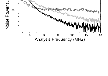
Figure 2: Individual laser noise for both lasers after interaction with the atomic sample. Circles: Laser 2 (full) and Laser 1 (hollow) at high power ($I=118$ mW/cm²); Lines: Laser 2 (black) and Laser 1 (gray) at low power ($I=25$ mW/cm²). Resolution Bandwidth (RBW) 1.0 MHz, Video Bandwidth (VBW) 3 kHz. Each curve is an average over 100 measurements.

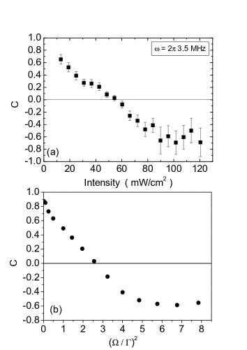
Figure 3: Variation of the correlation coefficient with laser intensity (per beam) for an analysis frequency of 3.5 MHz. (a) Experiment. RBW = 1 MHz and VBW = 3 kHz. Each point is an average over $6\times 10^{4}$ measurements. (b) Theory (as described in §4.2). $\Gamma$ is the spontaneous emission decay rate from the excited state ($\Gamma\approx 2\pi\times 6$ MHz). Other parameters are $\Delta_{1}=\Delta_{2}=2\pi\times 28.6$MHz, $b_{1}=b_{2}=0.08\Gamma$, $\gamma=0.02\Gamma$.

4 Results

4.1 Experimental results

The first step to measure the correlation between the fields transmitted by the atomic sample is to characterize the individual noise spectrum of each field. Before interaction, the intensity noise of the each ECDL is slightly above the standard quantum limit (SQL). In contrast, in spite of their narrow linewidths ($\sim$ 1 MHz), both lasers have large amounts of phase noise producing a very broad background spectrumZhang95 .

After interaction with the Doppler broadened atomic sample, the transmitted fields present high degrees of intensity fluctuations. The intensity noise spectra extend to frequencies as high as the Doppler width of the sampleYabuzaki91 . In the $D_{2}$ line of ${}^{85}Rb$, the energy separations of all excited levels are smaller than the Doppler width. Thus, in a vapor cell each laser excites all the atomic transitions allowed by dipole selection rules. The line strength of the $F\rightarrow F^{\prime}-$group is proportional to the mean value averaged by all possible dipole transitions belonging to this group. Substituting in the measured values, the $F=3\rightarrow F^{\prime}-$group has an effective dipole moment 1.12 times greater than the $F=2\rightarrow F^{\prime}-$group. If both fields have equal intensities (as is the case here), the Rabi frequency associated to Laser 2 will always be greater than the one associated to Laser 1. As a consequence, for a sufficiently high power, the transmitted intensity fluctuation of Laser 2 will be greater than that of Laser 1.

In Fig. 2 we present these noise spectra for both lasers at two different intensities measured after interaction with the atomic medium. For high power, the PN-to-AN conversion is considerably more efficient for the laser that is locked to the $F=3\rightarrow F^{\prime}-$group transition (laser 2), than for the laser locked to the $F=2\rightarrow F^{\prime}-$group transition. However, for a sufficiently low power, the efficiency of the PN-to-AN conversion is very low (and comparable) for both fields, and the noise power of Laser 2 can be lower than Laser 1 for small analysis frequencies. In this case, we have to keep in mind that absorption also plays a role, attenuating the mean field value and its fluctuations as well. The final result is a nonlinear character of the PN-to-AN conversion process.

Figure 4: (a)-(d) Experiment. Correlation coefficient spectra for various field intensities (in mW/cm²). (a) 13, (b) 61, (c) 96 (d) 118. The gray curve in (a) gives the same measurement without the vapor cell and for the highest intensity. RBW = 1.0 MHz, VBW = 3 kHz. Each curve is an average over 100 measurements. (e)-(h) Theoretical result for the correlation coefficient spectra for various Rabi frequencies ($\Omega$): (e) $\Omega=0.8\Gamma$, (f) $\Omega=1.6\Gamma$, (g) $\Omega=2.0\Gamma$ and (h) $\Omega=2.4\Gamma$. Other parameters are $\Delta_{1}=\Delta_{2}=2\pi\times 28.6$MHz, $b_{1}=b_{2}=0.08\Gamma$, $\gamma=0.02\Gamma$.

In Fig. 3(a) we show the experimental results for $C$ as the intensity is increased, for a fixed analysis frequency ($\omega=2\pi\times 3.5$ MHz). The first important point to notice is the high degree of correlation between the two fields after the sample, which can reach absolute values above 0.6. The other important feature is the clear transition from correlation to anti-correlation as the intensity is increased, passing through a nearly uncorrelated situation around 55 mW/cm².

We also measured the correlation spectral dependence which is shown in Figs. 4(a)-(d) for different intensities. We observe that the transition from correlation to anti-correlation occurs for all analysis frequencies from 2.5 MHz up to 14 MHz. Outside this spectral range, electronic noise prevents us from measuring the four power spectra necessary to evaluate $C$. At 14 MHz the correlation almost vanishes for all intensities. Nearly zero correlation is observed in the range from 50 to 60 mW/cm², with small fluctuations depending on the analysis frequency. Outside this range, the beams are clearly correlated over all the observed spectrum. Without the vapor cell in the beam pathway (gray curve in Fig. 4(a)), the correlation goes to zero for all analysis frequencies, as expected for two independent lasers.

The change in sign of the correlation coefficient can be understood as a consequence of the competition between two different processes occurring in a 3-level $\Lambda$ system: EIT and two-photon Raman transitions (both Stokes and anti-Stokes). At low intensities, EIT generates intensity correlations between the fields, since higher intensities of one field lead to an increase in the transparency of the medium to the second one. As the intensity is increased, the atomic transitions are power broadened and the system becomes saturated, so the Raman process (where one photon is absorbed from one field and emitted in the other) dominates the atomic excitation. Since in this case the decrease in one field’s intensity results in an increase of the other’s, it leads to an intensity anti-correlation between them. This will be clarified below, when we theoretically analyze the role of the optical detuning in a 3-level and in a 4-level atom.

4.2 Numerical results

In order to understand the influence of the various physical parameters involved in our experimental data, we explored our model in different ways. First, we analyzed the situation of a 3-level atom at rest, observing the dependence of correlation with the optical detuning, giving a physical interpretation for the change in sign of the correlation coefficient. Next, we studied the effect of the Rabi frequency on the correlation for the same situation, and in a second moment we performed the Doppler integration, observing the contribution of atoms of different velocity classes. Finally, we emphasize the contribution of the other excited atomic level presenting numerical results for the 4-level system. These results are compared to experimental data, showing good agreement.

The conversion of phase-noise to amplitude-noise is the main source of fluctuations observed in this system, but it is not sufficient to explain the passage from correlation to anti-correlation. We can have a better understanding by analyzing what happens to the correlation coefficient in the simplified model of a 3-level system at rest. In a $\Lambda$ configuration, the EIT resonance occurs in a frequency window (usually) much smaller than the natural linewidth associated to the optical transition. In other words, the two-photon Raman detuning — expressed as $\delta_{R}=\Delta_{2}-\Delta_{1}$ following the notation of Fig. 1 — should be zero and both fields must be nearly resonant with the (real) atomic state ($\Delta_{2}=\Delta_{1}=0$). If $\delta_{R}\neq 0$, linear absorption should occur. On the other hand, if both fields are off resonance with the excited level and $\delta_{R}=0$, the Raman process prevails. In this case, the atom can not absorb a photon from one of the two fields independently from the other. Only the two-photon stimulated Raman process, in which a photon absorbed from one field is re-emitted into the other field, can occur with high probability. We understand that the competition between these two processes is the basis of the observed change of sign for the correlation between pump and probe fields.

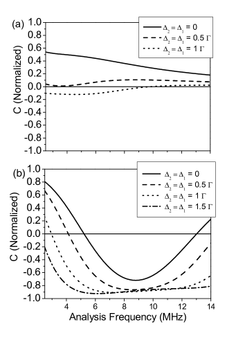
Figure 5: Numerical calculation of the correlation coefficient $C$ for a 3-level atom at rest as function of analysis frequency for different optical detunings. Two power ranges were analyzed: (a)$\Omega_{1}=0.1\Gamma,$ (b)$\Omega_{1}=\Gamma.$ Other parameters are $\Omega_{2}=1.12\Omega_{1}$, $b_{1}=b_{2}=0.08\Gamma,\,\gamma=0.02\Gamma$.

In Fig. 5 we show results that support our arguments. We numerically calculated the correlation coefficient $C$ as a function of analysis frequency for a 3-level atom at rest with constant Rabi frequency $\Omega$ and different values of the optical detuning $\Delta$. The calculations for low field intensity, presented in Fig. 5(a), give a nearly flat spectrum, with a reduction in the absolute value of correlation for higher analysis frequencies, following the behavior expected from the limited linewidth of the laser phase-noise. In these curves, we can see clearly the change from correlation to anti-correlation with an increasing detuning. This effect can be interpreted as the passage from the resonant EIT to a nonresonant Raman process, accompanied by a change in the photon statistics. For a higher intensity – Fig. 5(b) – the anti-correlation approaches its limit even for higher analysis frequencies. This can be seen as a consequence of the power broadening produced by the growth of intensity, increasing the contribution of the Raman process. Therefore, two mechanisms are present. While detuning reduces the EIT process and the intensity correlation, power broadening increases the Raman process and the anti-correlation.

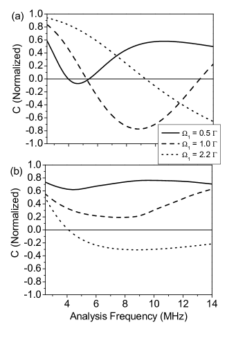
Figure 6: Numerical results of the correlation coefficient as a function of the analysis frequency for various Rabi frequencies ($\Omega$) in the case of a 3-level atom at rest (a) and for a Doppler broadened ensemble (b). $\Omega_{1}=0.5\Gamma$ (solid), $\Omega_{1}=1.0\Gamma$ (dashed), $\Omega_{1}=2.2\Gamma$ (dotted). $\Omega_{2}=1.12\Omega_{1},\,\Gamma\approx 2\pi\times 6$ MHz for ⁸⁵Rb, $b_{1}=b_{2}=0.08\Gamma,\,\gamma=0.02\Gamma$, $\Delta_{1}=\Delta_{2}=0$.

A more detailed study of the effect of the field intensity can be seen in Fig. 6(a). Here we analyze an atom at rest, with zero detuning. We can see the change from correlation to anticorrelation as a consequence of the increase in the Raman process, together with a broadening of the shape of the curve, demonstrated by an increase in the frequency for which the correlation changes sign. This can also be associated with power broadening of the atomic transition. Although we can see a few similarities with the experimental case, such as the change of in sign of the correlation coefficient $C$ with the incident intensity, the correlation changes rapidly with the analysis frequency, differently from what is observed in the experiment.

A better agreement to experimental data is obtained in Fig. 6(b), where the Doppler integration was performed. In fact, it is well known that in the $\Lambda$ configuration with co-propagating fields, atoms belonging to all different velocity classes contribute homogeneously to the signal, so if one is calculating the mean values, the Doppler integral can be avoided. However, for a phase diffusing field the optical detuning is a very important parameter and the Doppler width must be taken into account. One can see intuitively that a two-level atom at rest perfectly resonant with the field is almost insensitive to the field phase fluctuation, because it is at the maximum of the absorption curve. In contrast, if the atom is at the maximum slope of the absorption curve (or at the maximum of the dispersion curve), a small phase fluctuation will induce a large intensity fluctuation in the absorption profile and, as a consequence, in the transmitted light. This is the reason why the PN-to-AN conversion is associated to the real part of the atomic polarizationYabuzaki91 ; Walser94a . Thus, the Doppler integral accounts for the atoms having all the possible optical detunings and the PN-to-AN conversion in an atomic vapor is better reproduced. Furthermore, since the only source of noise in the theory is the fluctuating phases of the incident fields, this indicates that PN-to-AN conversion is the basic process behind our experimental observations.

With the integration over the Doppler width, we finally observe a curve that has a change from correlation to anti-correlation, but with a profile that changes slowly with the analysis frequency and doesn’t reach the high values of correlation calculated for an atom at rest. Fig. 6(b) still presents quantitative differences with respect to the experimental data. For example, we see that the passage to anti-correlation occurs for a broad range of analysis frequencies, higher than 4 MHz, while in the experiment, this passage occurs for smaller frequencies. As seen below, the inclusion of the fourth level in the model provides better agreement with the experimental data.

A better description of our system is obtained by including the second excited level $|0^{\prime}\rangle$ shown in Fig. 1 in the numerical calculation. In Fig. 4(e)-(h) we show results for the correlation coefficient $C$ as a function of the analysis frequency, for different values of Rabi frequencies, in the case of the 4-level system. In this situation, each transition has a different atomic dipole moment, so the field intensity is parameterized by a global constant $\Omega$, which is proportional to the field amplitude and the atomic dipole moment. We chose such a range of field intensities in order to adjust the theoretical results to the experimental curves. We notice that in the experimental situation the lasers were not locked to a real atomic transition corresponding to atoms at rest. Instead, we used a saturated absorption scheme to lock laser 2 on a cross-over peak, and the other laser was locked on the EIT resonance formed by the superposition of both. In this sense, the zero velocity atomic class was detuned approximately 28.6 MHz above the $F^{\prime}=3$ level. Since in the model the zero energy reference for the excited state is taken on the $|0\rangle$ state, we had to include an optical detuning in order to get a better agreement with the experimental curves. If this optical detuning is not considered, the anti-correlation is significantly reduced (in absolute value), but the spectral feature of $C(\omega)$ does not change appreciably. We can observe the change from correlation to anti-correlation for increasing Rabi frequencies, and a good qualitative agreement of the spectral plots, especially for higher Rabi frequencies.

In order to compare these results with our experimental data, we also calculated the variation of $C$ with the Rabi frequency for a fixed analysis frequency ($\omega=2\pi\times 3.6$ MHz). This is shown in Fig. 3(b). We clearly see a change in sign for the correlation between pump and probe fields as in the experimental case, with a good agreement to the experimental data.

Finally, we now briefly comment the role of the laser linewidth on the sign of $C(\omega)$. In light of the previous analysis, the correlated fields in the EIT situation become anti-correlated if either the optical detuning is increased or the atomic transition becomes power broadened. We checked numerically that if the laser linewidth increases so much that it is comparable to (or higher than) the excited state decay rate $\Gamma$, the correlation between fields tends to change sign. The physical mechanism is totally analogous since the effect of laser broadening is to produce more sidebands in frequencies that are not perfectly resonant with the EIT transition, favoring the Raman process. We also confirmed that in a 3-level system this effect is more pronounced than in a 4-level atom. In other words, for the same laser linewidth and power, $C(\omega)$ is more negative in the case of a 3-level system than in the 4-level situation. Consider that the carrier laser frequency is resonant with one of the excited levels. In the 3-level atom, the laser side bands will be far off resonance with the atomic transitions, producing pure Raman transitions, while in a 4-level atom, these side bands approach the other excited state forming a second $\Lambda$ system (eventually becoming resonant), so both processes tend to compensate each other.

It is important now to address some significant differences between the experimental and theoretical results presented in Fig. 4. The main discrepancy observed is that the theoretical curves do not show the fast decay of the correlation as the analysis frequency is increased. Discrepancies in the higher frequency domain can be accounted for by the amplifier gain and the reduction of the signal-to-noise ratio of our detection. Moreover, in the experimental curves, the Spectrum Analyzer measures the noise power centered at a chosen frequency and averaged over a Resolution Bandwidth of 1 MHz. In the model, the analyzer is supposed to be ideal.

Differences may also come from the simplicity of our model. In the Doppler broadened ⁸⁵Rb $D_{2}$ transition, the excited level is composed of 4 states, namely $F^{\prime}=$ 1 — 4, two of which (the $F^{\prime}=2$ and $F^{\prime}=3$ considered in the model) contribute to the $\Lambda$ level-schemes. However, three of the four levels contribute to the each of the single-photon optical transitions, which give rise to the PN-to-AN process. These are crucial for the $S_{11}(\omega)$ and $S_{22}(\omega)$ spectra – used for determining the correlation coefficient $C$. An important point comes from the absence of the $F^{\prime}=4$ level in calculating $S_{22}$, because this is the strongest optical (and closed) transition and is the main responsible for the increase in the noise power seen in Fig. 2 for the Laser 2. A similar reasoning is valid for the $F^{\prime}=1$ level for the case of Laser 1. Furthermore, in Fig. 3 we see that, in the experiment, the laser intensity corresponding to the change in sign for the correlation coefficient is much higher than the saturation intensity. In the theoretical case, the Rabi frequency necessary for this change in sign is approximately twice the saturation. We remember that the model is based on the assumption of an optically thin medium, which is not necessarily true in the experiment. So, the real field intensity required to overcome the EIT effect and introduce anti-correlations via Raman transitions may be considerably higher.

The way we model the laser noise may also give rise to discrepancies with the experiment. We considered that the lasers have perfect Lorentzian lineshapes, which have slow-decay spectral wings. A more realistic model for a diode laser, on the other hand, should include a gaussian cutoff to the Lorentzian lineshapeDixit80 ; Ritsch90 ; Anderson90a , so that the wings of the field spectra fall much faster than for a pure Lorentzian shape. This comes from the fact that the amplitude and phase fluctuations are strongly coupled in a solid state laserHenry82 ; Henry83 . Noise spectra, from PN-to-AN conversion, will also depend on the shape of the phase noise spectra. This gaussian cutoff may account for the smaller absolute values of correlation obtained in the experiment, in comparison with the theoretical data, as well as the faster reduction of the correlation for higher analysis frequencies. Models different from the one adopted here may give a better agreement to the experimental data, but their implementation is a much harder task using the present framework. Nevertheless, the simplified Lorentzian description already gives us a good understanding of the physical processes involved, and quite good agreement to the experimental data.

5 Conclusions

In summary, we have shown that the propagation of two initially independent fields generating EIT in a vapor cell results in a high degree of correlation between the fields for a broad range of analysis frequencies. We also observed the transition from intensity correlation to anti-correlation as the field intensities are increased. We explain these observations in terms of conversion of phase noise to amplitude noise by the atomic medium, and the opposite behaviors of the EIT and Raman resonances. We develop a more detailed calculation to support this claim. In this way, these observations reveal new basic features of the EIT effect, and stress again how deeply EIT can affect the excitation fields.

References

- (1) L.V. Hau, S.E. Harris, Z. Dutton, C.H. Behroozi, Nature 397(18), 594 (1999)
- (2) C. Liu, Z. Dutton, C.H. Behroozi, L.V. Hau, Nature 409, 490 (2001)
- (3) M. Bajcsy, A.S. Zibrov, M.D. Lukin, Nature 426, 638 (2003)
- (4) C.V.d. Wal, M. Eisaman, A. Andre, R. Walsworth, D. Phillips, A. Zibrov, M. Lukin, Science 301(i5630), 196 (2003)
- (5) R. Beausoleil, W. Munro, D. Rodrigues, T. Spiller, J. of Mod. Optics 51, 2441 (2004)
- (6) C. Garrido-Alzar, L.S.D. Cruz, J.G. Aguirre-Gómez, M.F. Santos, P. Nussenzveig, Europhys. Lett. 61, 485 (2003)
- (7) A.F. Huss, R. Lammegger, C. Neureiter, E.A. Korsunsky, L. Windholz, Phys. Rev. Lett. 93, 223601 (2004)
- (8) P. Barberis-Blostein, N. Zagury, Phys. Rev. A 70, 053827 (2004)
- (9) T. Yabuzaki, T. Mitsui, U. Tanaka, Phys. Rev. Lett 67(18), 2453 (1991)
- (10) K. Petermann, Laser Diode Modulation and Noise, Vol. 73 (Kluwer Academic Publishers, 1991)
- (11) T.C. Zhang, J.P. Poizat, P. Grelu, J.F. Roch, P. Grangier, F. Martin, A. Bramati, V. Jost, M.D. Levenson, E. Giacobino, Quamt. Semiclass. Opt. 7, 601 (1995)
- (12) R. Walser, P. Zoller, Phys. Rev. A 49(6), 5067 (1994)
- (13) J.C. Camparo, G. Coffer, Phys. Rev. A 59(1), 728 (1999)
- (14) D.H. McIntyre, C.E. Fairchild, J. Cooper, R. Walser, Opt. Lett. 18(21), 1816 (1993)
- (15) M. Bahoura, A. Clairon, Opt. Lett. 26(12), 926 (2001)
- (16) R. Walser, J. Cooper, P. Zoller, Phys. Rev. A 50(5), 4303 (1994)
- (17) M.H. Anderson, R.D. Jones, J. Cooper, S.J. Smith, D.S. Elliott, H. Ritsch, P. Zoller, Phys. Rev. Lett 64(12), 1346 (1990)
- (18) M.H. Anderson, R.D. Jones, J. Cooper, S.J. Smith, D.S. Elliott, H. Ritsch, P. Zoller, Phys. Rev. A 42(11), 6690 (1990)
- (19) H. Ritsh, P. Zoller, J. Cooper, Phys. Rev. A 41(5), 2653 (1990)
- (20) M. Martinelli, P. Valente, H. Failache, D. Felinto, L.S. Cruz, P. Nussenzveig, A. Lezama, Phys. Rev. A 69, 043809 (2004)
- (21) V.A. Sautenkov, Y.V. Rostovtsev, M.O. Scully, Phys. Rev. A 72, 065801 (2005)
- (22) G.O. Ariunbold, V.A. Sautenkov, Y.V. Rostovtsev, M.O. Scully, arXiv:quant-ph p. /0603025 (2005)
- (23) J. Camparo, J. Coffer, J. Townsend, J. Opt. Soc. Am. B 22(3), 521 (2005)
- (24) C.W. Gardiner, Handbook of Stochastic Methods (Springer-Verlag Berlin Heidelberg, 1983)
- (25) S.N. Dixit, P. Zoller, P. Lambropoulos, Phys. Rev. A 21(4), 1289 (1980)
- (26) C.H. Henry, IEEE J. of Quant. Eletron. QE-18(2), 259 (1982)
- (27) C.H. Henry, IEEE J. of Quant. Eletron. QE-19(9), 1391 (1983)