Abstract

By using the Lindblad theory for open quantum systems, an analytical expression of the tunneling probability through an inverted parabola is obtained. This penetration probability depends on the environment coefficients. It is shown that the tunneling probability increases with the dissipation and the temperature of the thermal bath.

PACS numbers: 03.65.Bz, 05.30.-d, 05.40.Jc

(a) e-mail address: isar@theory.nipne.ro

1 Introduction

Quantum tunneling with dissipation has been intensively investigated in the last two decades [1–12]. Very interesting is the discussion whether the dissipation suppresses or enhances the quantum tunneling. Caldeira and Leggett [1, 2] concluded that dissipation tends to suppress quantum tunneling. Using a different method, Schmid obtained similar results in Ref. [13]. Widom and Clark [14] considered a parabolic potential barrier and found that dissipation enhances tunneling. Bruinsma and Bak [15] also considered tunneling through a barrier and found that at zero temperature the tunneling rate can be either increased or decreased by dissipation. Leggett [16] considered tunneling in the presence of an arbitrary dissipation mechanism and found that, normally, dissipation impedes tunneling, but he also found an anomalous case in which dissipation assists the tunneling process. Razavy [17] considered tunneling in a symmetric double-well potential and concluded that dissipation can inhibit or suppress tunneling. Fujikawa et al. [18] also considered tunneling in a double-well potential and found an enhancement of tunneling. Harris [19] calculated the tunneling out of a metastable state in the presence of an environment at zero temperature and found that quantum tunneling is enhanced by dissipation. In [20], Yu considered the tunneling problem in an Ohmic dissipative system with inverted harmonic potential and he showed that while the dissipation tends to suppress the tunneling, the Brownian motion tends to enhance it. In a series of papers [21, 22], Ankerhold, Grabert and Ingold have studied real time dynamics of a quantum system with a potential barrier coupled to a heat bath environment, employing the path integral approach. The conclusion drawn from these papers is that different authors have studied different problems using different methods. They obtained results which in many cases present an evident contradiction.

In the present paper we study the tunneling in the presence of a dissipative environment in the framework of the Lindblad theory for open quantum systems, based on completely positive dynamical semigroups [23–25]. We extend the work done in some previous papers [26, 27]. In [27] a similar problem was treated by using the path integral method and numerical calculations. Our study can be applied to problems of nuclear fragmentation, fission and fusion, considered as a tunneling process through the nuclear barrier defined in the space of collective coordinates, like charge and mass asymmetry or the distance between the fission fragments.

For the inverted harmonic potential, the tunneling problem in the framework of the Lindblad theory can be solved exactly. In Sec. 2 we write the basic equations of the Lindblad theory for open quantum systems and give results for the coordinate and momentum expectation values and variances for the damped inverted harmonic oscillator. Then in Sec. 3 we consider the penetration of a Gaussian wave packet through the potential barrier and define the penetration probability. In Sec. 4 we analyze its dependence on various dimensionless parameters which enter the theory and show that the probability increases with the dissipation and the temperature of the thermal bath. A summary is given in Sec. 5.

2 Quantum Markovian master equation in
Lindblad theory

The simplest dynamics for an open system which describes an irreversible process is a semigroup of transformations introducing a preferred direction in time [23–25]. In Lindblad’s axiomatic formalism of introducing dissipation in quantum mechanics, the usual von Neumann-Liouville equation ruling the time evolution of closed quantum systems is replaced by the following quantum master equation for the density operator $\rho(t)$ in the Schrödinger picture [24], which is the most general Markovian evolution equation preserving the positivity, hermiticity and unit trace of $\rho$:

$${d\rho(t)\over dt}=-{i\over\hbar}[H,\rho(t)]+{1\over 2\hbar}\sum_{j}(2V_{j}\rho(t)V_{j}^{\dagger}-V_{j}^{\dagger}V_{j}\rho(t)-\rho(t)V_{j}^{\dagger}V_{j}).$$ (1)

Here $H$ is the Hamiltonian operator of the system; $V_{j},$ $V_{j}^{\dagger}$ are bounded operators on the Hilbert space of the Hamiltonian and model the effect of the environment. We make the basic assumption that the general form (1) of the master equation with a bounded generator is also valid for an unbounded generator.

As usual, we define the two possible environment operators $V_{1}$ and $V_{2},$ which are assumed linear in momentum $p$ and coordinate $q,$ as follows [28, 29]:

$$V_{j}=a_{j}p+b_{j}q,~{}j=1,2,$$ (2)

with $a_{j},b_{j}$ complex numbers. The Hamiltonian $H$ is chosen of the general form

$$H=H_{0}+{\mu\over 2}(qp+pq),~{}~{}~{}H_{0}={1\over 2m}p^{2}+U(q),$$ (3)

where $U(q)$ is the potential. With these choices and with the notations

$$D_{qq}={\hbar\over 2}\sum_{j=1,2}{|a_{j}|}^{2},D_{pp}={\hbar\over 2}\sum_{j=1,2}{|b_{j}|}^{2},D_{pq}=D_{qp}=-{\hbar\over 2}{\rm Re}\sum_{j=1,2}a_{j}^{*}b_{j},\lambda=-{\rm Im}\sum_{j=1,2}a_{j}^{*}b_{j},$$ (4)

where $a_{j}^{*}$ and $b_{j}^{*}$ denote the complex conjugate of $a_{j}$ and $b_{j},$ respectively, the master equation (1) takes the following form [28, 29]:

$${d\rho\over dt}=-{i\over\hbar}[H_{0},\rho]-{i\over 2\hbar}(\lambda+\mu)[q,\rho p+p\rho]+{i\over 2\hbar}(\lambda-\mu)[p,\rho q+q\rho]$$

$$-{D_{pp}\over{\hbar}^{2}}[q,[q,\rho]]-{D_{qq}\over{\hbar}^{2}}[p,[p,\rho]]+{D_{pq}\over{\hbar}^{2}}([q,[p,\rho]]+[p,[q,\rho]]).~{}~{}~{}~{}$$ (5)

Here the quantum diffusion coefficients $D_{pp},D_{qq},$ $D_{pq}$ and the dissipation constant $\lambda$ satisfy the following fundamental constraints [28, 29]: $D_{pp}>0,D_{qq}>0$ and

$$D_{pp}D_{qq}-D_{pq}^{2}\geq{{\lambda}^{2}{\hbar}^{2}\over 4}.$$ (6)

In the particular case when the asymptotic state is a Gibbs state

$$\rho_{G}(\infty)=e^{-{H_{0}\over kT}}/{\rm Tr}e^{-{H_{0}\over kT}},$$ (7)

the coefficients for a harmonic oscillator potential have the following form [28, 29]:

$$D_{pp}={\lambda+\mu\over 2}\hbar m\omega\coth{\hbar\omega\over 2kT},~{}~{}D_{qq}={\lambda-\mu\over 2}{\hbar\over m\omega}\coth{\hbar\omega\over 2kT},~{}~{}D_{pq}=0,$$ (8)

where $T$ is the temperature of the thermal bath. The fundamental constraint (6) is satisfied only if $\lambda>\mu.$

In the following we denote by $\sigma_{AA}$ the dispersion (variance) of the operator $A$, i.e. $\sigma_{AA}=<A^{2}>-<A>^{2},$ where $<A>\equiv\sigma_{A}={\rm Tr}(\rho A)$ is the expectation value of the operator $A$ and ${\rm Tr}\rho=1.$ By $\sigma_{AB}=1/2<AB+BA>-<A><B>$ we denote the correlation of the operators $A$ and $B.$

From the master equation (5) we obtain the following equations of motion for the expectation values and variances of coordinate and momentum:

$${d\sigma_{q}(t)\over dt}=-(\lambda-\mu)\sigma_{q}(t)+{1\over m}\sigma_{p}(t),$$ (9)

$${d\sigma_{p}(t)\over dt}=-<{dU(q)\over dq}>-(\lambda+\mu)\sigma_{p}(t)$$ (10)

and, respectively,

$${d\sigma_{qq}(t)\over dt}=-2(\lambda-\mu)\sigma_{qq}(t)+{2\over m}\sigma_{pq}(t)+2D_{qq},$$ (11)

$${d\sigma_{pp}\over dt}=-2(\lambda+\mu)\sigma_{pp}(t)-<{dU(q)\over dq}p+p{dU(q)\over dq}>+2<{dU(q)\over dq}>\sigma_{p}(t)+2D_{pp},$$ (12)

$${d\sigma_{pq}(t)\over dt}=-<{dU(q)\over dq}q>+<{dU(q)\over dq}>\sigma_{q}(t)+{1\over m}\sigma_{pp}(t)-2\lambda\sigma_{pq}(t)+2D_{pq}.$$ (13)

For the harmonic oscillator with the potential $U(q)=m\omega^{2}q^{2}/2,$ the solutions of these equations of motion are obtained in Refs. [28, 29]. In this paper we consider the tunneling through a potential barrier given by an inverted harmonic potential (inverted parabola) with

$$U(q)=-{m\omega^{2}\over 2}q^{2}.$$ (14)

The Hamiltonian $H_{0}$ in equation (3) with the potential (14) can be regarded as the Hamiltonian of a harmonic oscillator with an imaginary frequency $i\omega$ and the equations of motion (9)–(13) for this potential are formally obtained by performing the replacement $\omega\to i\omega$ in the corresponding equations for the harmonic oscillator. These equations of motions can be solved by using the same method as in references [28, 29] for the harmonic oscillator. Contrary to the situation of the harmonic oscillator, where we have two cases, overdamped and underdamped, for the inverted parabola such a distinction does not exist. The solutions for the expectation values and variances of coordinate and momentum coincide formally with the solutions corresponding to the overdamped case of the harmonic oscillator. For the expectation value of the coordinate and momentum we obtain with $\nu\equiv\sqrt{\omega^{2}+\mu^{2}}:$

$$\sigma_{q}(t)=e^{-\lambda t}((\cosh\nu t+{\mu\over\nu}\sinh\nu t)\sigma_{q}(0)+{1\over m\nu}\sinh\nu t\sigma_{p}(0)),$$ (15)

$$\sigma_{p}(t)=e^{-\lambda t}({m\omega^{2}\over\nu}\sinh\nu t\sigma_{q}(0)+(\cosh\nu t-{\mu\over\nu}\sinh\nu t)\sigma_{p}(0)).$$ (16)

In the following we also need the solution for the variance $\sigma_{qq}$, which is given by:

$$\sigma_{qq}(t)={e^{-2\lambda t}\over 2\nu^{2}}\{\Delta_{qq}[(\mu^{2}+\nu^{2})\cosh 2\nu t+2\mu\nu\sinh 2\nu t+\omega^{2}]+{\Delta_{pp}\over m^{2}}(\cosh 2\nu t-1)$$

$$+{2\over m}\Delta_{pq}(\mu\cosh 2\nu t+\nu\sinh 2\nu t-\mu)\}+\sigma_{qq}(\infty),~{}~{}~{}~{}~{}~{}~{}~{}~{}~{}~{}~{}~{}~{}~{}~{}$$ (17)

where $\Delta_{qq}=\sigma_{qq}(0)-\sigma_{qq}(\infty),$ $\Delta_{pp}=\sigma_{pp}(0)-\sigma_{pp}(\infty),$ $\Delta_{pq}=\sigma_{pq}(0)-\sigma_{pq}(\infty)$ and

$$\sigma_{qq}(\infty)={1\over 2m^{2}\lambda(\lambda^{2}-\omega^{2}-\mu^{2})}(m^{2}(2\lambda(\lambda+\mu)-\omega^{2})D_{qq}+D_{pp}+2m(\lambda+\mu)D_{pq}),$$ (18)

$$\sigma_{pp}(\infty)={1\over 2\lambda(\lambda^{2}-\omega^{2}-\mu^{2})}((m\omega)^{2}\omega^{2}D_{qq}+(2\lambda(\lambda-\mu)-\omega^{2})D_{pp}+2m\omega^{2}(\lambda-\mu)D_{pq}),$$ (19)

$$\sigma_{pq}(\infty)={1\over 2m\lambda(\lambda^{2}-\omega^{2}-\mu^{2})}((\lambda+\mu)(m\omega)^{2}D_{qq}+(\lambda-\mu)D_{pp}+2m(\lambda^{2}-\mu^{2})D_{pq}).$$ (20)

Note that in the case $\lambda>\nu,$ $\sigma_{q}(t\to\infty)=\sigma_{p}(t\to\infty)=0$ and $\sigma_{qq}(t\to\infty)=\sigma_{qq}(\infty).$ In the case $\lambda<\nu$, $\sigma_{q}(t\to\infty),\sigma_{p}(t\to\infty)\to\pm\infty$ and $\sigma_{qq}(t\to\infty)=\infty.$

3 Tunneling through an inverted parabola

In order to calculate the tunneling probability through the inverted harmonic potential (14), we assume that initially the wave function of the system is a Gaussian wave packet centered at the left of the peak of the potential at $q=0,$ $\sigma_{q}(0)<0$, with a momentum $\sigma_{p}(0)>0$ towards the potential barrier peak:

$$\psi(q)={1\over(2\pi\sigma_{qq}(0))^{1/4}}\exp[-{1\over 4\sigma_{qq}(0)}(q-\sigma_{q}(0))^{2}+{i\over\hbar}\sigma_{p}(0)q].$$ (21)

Then the corresponding initial probability density is given by:

$$\rho(q,t=0)={1\over(2\pi\sigma_{qq}(0))^{1/2}}\exp[-{1\over 2\sigma_{qq}(0)}(q-\sigma_{q}(0))^{2}].$$ (22)

Like in [30]–[32], we can transform the master equation (5) for the density operator of a particle moving in the potential (14) of an inverted parabola into the following Fokker-Planck equation satisfied by the Wigner distribution function $W(q,p,t):$

$${\partial W\over\partial t}=-{p\over m}{\partial W\over\partial q}-m\omega^{2}q{\partial W\over\partial p}+(\lambda-\mu){\partial\over\partial q}(qW)+(\lambda+\mu){\partial\over\partial p}(pW)$$

$$+D_{qq}{\partial^{2}W\over\partial q^{2}}+D_{pp}{\partial^{2}W\over\partial p^{2}}+2D_{pq}{\partial^{2}W\over\partial p\partial q}.~{}~{}~{}~{}~{}~{}~{}~{}~{}~{}~{}~{}~{}~{}~{}~{}~{}~{}~{}$$ (23)

For an initial Gaussian Wigner function, the solution of Eq. (23) is

$$W(q,p,t)={1\over 2\pi\sqrt{\sigma(t)}}~{}~{}~{}~{}~{}~{}~{}~{}~{}~{}~{}~{}~{}~{}~{}~{}~{}~{}~{}~{}~{}~{}~{}~{}~{}~{}~{}~{}~{}~{}~{}~{}~{}$$

$$\times\exp\{-{1\over 2\sigma(t)}[\sigma_{pp}(t)(q-\sigma_{q}(t))^{2}+\sigma_{qq}(t)(p-\sigma_{p}(t))^{2}-2\sigma_{pq}(t)(q-\sigma_{q}(t))(p-\sigma_{p}(t))]\},$$ (24)

which represents the most general mixed squeezed states of Gaussian form. Here $\sigma_{q}(t),$ $\sigma_{p}(t)$ and $\sigma_{qq}(t),$ $\sigma_{pp}(t),$ $\sigma_{pq}(t)$ are the expectation values and, respectively, the variances corresponding to the inverted parabola as given partly in Eqs. (15)–(17) and

$$\sigma(t)=\sigma_{qq}(t)\sigma_{pp}(t)-\sigma_{pq}(t)^{2}.$$ (25)

Since the dynamics is quadratic, then according to known general results, the initial Wigner function remains Gaussian. The density matrix can be obtained by the inverse Fourier transform of the Wigner function:

$$<q|\rho|q^{\prime}>=\int dp\exp({i\over\hbar}p(q-q^{\prime}))W({q+q^{\prime}\over 2},p,t).$$ (26)

Using Eq. (24), we get for the density matrix the following time evolution:

$$<q|\rho|q^{\prime}>=({1\over 2\pi\sigma_{qq}(t)})^{1\over 2}\exp[-{1\over 2\sigma_{qq}(t)}({q+q^{\prime}\over 2}-\sigma_{q}(t))^{2}~{}~{}~{}~{}~{}~{}~{}~{}~{}$$

$$-{1\over 2\hbar^{2}}(\sigma_{pp}(t)-{\sigma_{pq}^{2}(t)\over\sigma_{qq}(t)})(q-q^{\prime})^{2}+{i\sigma_{pq}(t)\over\hbar\sigma_{qq}(t)}({q+q^{\prime}\over 2}-\sigma_{q}(t))(q-q^{\prime})+{i\over\hbar}\sigma_{p}(t)(q-q^{\prime})].$$ (27)

The initial Gaussian density matrix also remains Gaussian, centered around the classical path, i. e. $\sigma_{q}(t)$ and $\sigma_{p}(t)$ give the average time-dependent location of the system along its trajectory in phase space. The wave function starts as a Glauber wave packet at $t=0$ on the left-hand side of the barrier and evolves as a mixed squeezed state at a later time. By putting $q^{\prime}=q$ in Eq. (27), we obtain the following probability density of finding the particle in the position $q$ at the moment $t$:

$$\rho(q,t)={1\over(2\pi\sigma_{qq}(t))^{1/2}}\exp[-{1\over 2\sigma_{qq}(t)}(q-\sigma_{q}(t))^{2}].$$ (28)

This is a Gaussian distribution centered at $\sigma_{q}(t),$ which describes the classical trajectory of a particle initially at $\sigma_{q}(0)$, with initial momentum $\sigma_{p}(0)$ and variance $\sigma_{qq}(t).$

Using Eq. (28), the probability for the particle to pass to the right of position $q$ at time $t$ is given by

$$P(q,t)=\int_{q}^{\infty}\rho(q^{\prime},t)dq^{\prime}=\int_{q}^{\infty}{1\over\sqrt{2\pi\sigma_{qq}(t)}}\exp(-{(q^{\prime}-\sigma_{q}(t))^{2}\over 2\sigma_{qq}(t)})dq^{\prime}.$$ (29)

We define the tunneling probability $P(t)$ as the probability for the particle to be at the right of the peak at $q=0$ (beyond the barrier top): $P(t)=P(q=0,t).$ We obtain

$$P(t)={1\over\sqrt{\pi}}\int_{-\sigma_{q}(t)\over\sqrt{2\sigma_{qq}(t)}}^{\infty}e^{-u^{2}}du={1\over 2}(1-{\rm erf}(-{\sigma_{q}(t)\over\sqrt{2\sigma_{qq}(t)}})),$$ (30)

where ${\rm erf}(x)$ is the error function with ${\rm erf}(x)={-\rm erf}(-x)$ and erf($\infty$)=1.

From Eq. (30) we see that the probability $P(t)$ depends only upon the classical motion of the average value of coordinate (wave packet center) and the spreading of the wave packet in the direction of the barrier. The final tunneling probability (barrier penetrability) is given by taking the limit $t\to\infty$ in $P(t)$. In the present calculations we ignore the fact that a part of the wave packet has already tunneled through the barrier at $t=0.$ In general, this probability has a negligible value, but, in principle, in order to find the net penetration probability, it should be subtracted from the tunneling probability at time $t.$

4 Evaluation of the penetration probability and
analysis in dimensionless variables

We will show that since $\sigma_{q}(t)$ and $\sqrt{\sigma_{qq}(t)}$ are both proportional to the same exponential factor as time approaches infinity, their ratio in Eq. (30) approaches a finite limit, which determines the final tunneling probability. Indeed, as $t\to\infty,$ we see from Eqs. (15) and (17) that $\sigma_{q}(t)$ and $\sigma_{qq}(t)$ behave like

$$\sigma_{q}(t)\to{e^{-(\lambda-\nu)t}\over 2m\nu}\delta$$ (31)

and

$$\sigma_{qq}(t)\to({e^{-(\lambda-\nu)t}\over 2m\nu})^{2}\Delta+\sigma_{qq}(\infty),$$ (32)

where we have denoted

$$\delta\equiv m(\mu+\nu)\sigma_{q}(0)+\sigma_{p}(0)$$ (33)

and

$$\Delta\equiv m^{2}(\mu+\nu)^{2}\Delta_{qq}+\Delta_{pp}+2m(\mu+\nu)\Delta_{pq}.$$ (34)

Then we obtain the following finite limit as $t\to\infty:$

$${\sigma_{q}(t)\over\sqrt{\sigma_{qq}}}\to{\delta\over\sqrt{\Delta}}$$ (35)

if $\lambda<\nu$ (and the limit $0$ if $\lambda>\nu$) and, therefore, the expression (30) leads to the final penetration probability $(P=P(t\to\infty))$

$$P={1\over 2}(1-{\rm erf}(-{\delta\over\sqrt{2\Delta}}))$$ (36)

if $\lambda<\nu$ and $P=1/2$ if $\lambda>\nu.$ In the case $\lambda>\nu,$ $\sigma_{q}(t)\to 0$ if $t\to\infty$, that is, the system is located around the barrier, $\sigma_{qq}(t)$ tends to a finite value $\sigma_{qq}(\infty)$ for any initial kinetic energy and in this case $P(t)=1/2.$ Let us consider the other case $\lambda<\nu$. For $\delta=0$ the trajectory tends to the top of the potential barrier and if $\delta$ is different from 0, then $\sigma_{q}(t)$ tends to $\infty$ or $-\infty.$ The trajectory which starts on the left-hand side of the barrier ($\sigma_{q}(0)<0$) with a positive initial momentum $\sigma_{p}(0)>0$ will stay on the same side for $\delta<0$ (and then $\sigma_{q}(\infty)\to-\infty$) and will cross the barrier for $\delta>0,$ i. e. if the initial kinetic energy allows to overcome the barrier (and then $\sigma_{q}(\infty)\to\infty$). For a general $\mu$ and any $\lambda<\nu,$ the particle crosses the barrier when $\sigma_{p}(0)>-m(\mu+\nu)\sigma_{q}(0)$ and will stay on the same side when $\sigma_{p}(0)<-m(\mu+\nu)\sigma_{q}(0).$ The barrier penetrability is larger than 1/2 if the particle classically can overcome the top of the barrier, it is smaller than 1/2 if the particle cannot cross the barrier and it tends to 1/2 if the position uncertainty $\sigma_{qq}$ is very large.

For $\mu=0,$ the values of $\Delta$ and $\delta$ become ($\nu=\omega$):

$$\delta_{0}=m\omega\sigma_{q}(0)+\sigma_{p}(0)$$ (37)

and

$$\Delta_{0}=m^{2}\omega^{2}\sigma_{qq}(0)+\sigma_{pp}(0)+2m\omega\sigma_{pq}(0)-{m^{2}\omega^{2}D_{qq}+D_{pp}+2m\omega D_{pq}\over\lambda-\omega}.$$ (38)

The particle crosses the barrier if $\sigma_{p}(0)>-m\omega\sigma_{q}(0)$ and $\lambda<\omega.$ In this case, if $\lambda$ increases, then the ratio $\delta_{0}/(2\Delta_{0})^{1/2}$ and the penetration probability $P$ decreases. This means that if dissipation increases, then the probability $P$ decreases up to a value of 1/2. If $\sigma_{p}(0)<-m\omega\sigma_{q}(0),$ the particle can not cross the barrier. In this case the penetration probability $P$ increases with the dissipation $\lambda$ up to 1/2. At $\lambda\geq\omega$ the wave packet sticks in the barrier region.

We now introduce the dimensionless variables: $z$ the scaled initial position, $v$ the scaled initial momentum, $\epsilon$ the scaled dissipation coefficient and $r$ the scaled inverse wave packet size, defined as follows:

$$z={\sigma_{q}(0)\over\sqrt{\sigma_{qq}(0)}},~{}~{}v={\sigma_{p}(0)\over m\omega\sigma_{q}(0)},~{}~{}\epsilon={\lambda\over\omega},~{}~{}r={\sqrt{\displaystyle{\hbar\over 2m\omega}}\over\sqrt{\sigma_{qq}(0)}}.$$ (39)

With these notations and considering a thermal bath modeled by the coefficients of the form (8), the penetration probability takes the following form for the case $\mu=0$:

$$P_{\mu=0}={1\over 2}(1-{\rm erf}(-{\delta_{0}\over\sqrt{2\Delta_{0}}}))={1\over 2}(1-{\rm erf}(-{z(1+v)\over\sqrt{2}\displaystyle{\sqrt{1+r^{4}-{2\epsilon\over\epsilon-1}r^{2}\coth{\hbar\omega\over 2kT}}}})).$$ (40)

We took into account that

$$\sigma_{qq}(0)\sigma_{pp}(0)=\hbar^{2}/4,~{}~{}~{}~{}(\sigma_{pq}(0)=0).$$ (41)

If $\mu=0,$ then we have $0<\epsilon<1.$

For $\mu\neq 0,$ in the case of a thermal bath, the expression (34) takes the form $(\sigma_{pq}(0)=0)$

$$\Delta=m^{2}(\mu+\nu)^{2}\sigma_{qq}(0)+\sigma_{pp}(0)$$

$$-{\hbar m\over\omega}\{\mu(\mu+\nu)+{\omega^{2}[\lambda^{2}+\lambda(\mu+\nu)+\mu\nu]\over\lambda^{2}-\omega^{2}-\mu^{2}}\}\coth{\hbar\omega\over 2kT}.$$ (42)

With the notations (39) and introducing also the notation

$$\gamma={\mu\over\omega},$$ (43)

the penetration probability takes the following form:

$$P_{\mu\neq 0}={1\over 2}(1-{\rm erf}(-{\delta\over\sqrt{2\Delta}})),$$ (44)

with

$${\delta\over\sqrt{\Delta}}={z(\gamma+\sqrt{1+\gamma^{2}}+v)\over[(\gamma+\sqrt{1+\gamma^{2}})^{2}+r^{4}-2(\gamma+\sqrt{1+\gamma^{2}})\displaystyle{{{(\epsilon^{2}-\gamma^{2})\sqrt{1+\gamma^{2}}+\epsilon\over\epsilon^{2}-\gamma^{2}-1}}r^{2}\coth{\hbar\omega\over 2kT}}]^{1/2}}.$$ (45)

If $\mu\neq 0$, the inequalities $\lambda>\mu$ (see Eq. (8) and $\lambda<\nu$ lead to the following restrictions on the dimensionless variables:

$$\gamma<\epsilon<\sqrt{1+\gamma^{2}}.$$ (46)

The initial energy of the particle associated with the Gaussian wave packet (21) is

$$E=<H>|_{t=0}={1\over 2m}\sigma_{pp}(0)-{m\omega^{2}\over 2}\sigma_{qq}(0)+{1\over 2m}\sigma^{2}_{p}(0)-{m\omega^{2}\over 2}\sigma^{2}_{q}(0)+\mu\sigma_{p}(0)\sigma_{q}(0)$$ (47)

and in terms of the dimensionless variables (39) it looks

$$E={\hbar\omega\over 4r^{2}}[r^{4}-1+z^{2}(v^{2}-1)]+{\hbar\mu\over 2}{z^{2}v\over r^{2}}.$$ (48)

If $E<0$ it is a sub-barrier initial energy and if $E>0$ it is an energy above the barrier. In terms of the same dimensionless variables, the condition that a classical particle does not have enough initial kinetic energy to pass the potential barrier can be written:

$$v>-1,~{}~{}~{}~{}~{}{\rm if}~{}\mu=0$$ (49)

and

$$v>-(\gamma+\sqrt{1+\gamma^{2}}),~{}~{}~{}~{}~{}{\rm if}~{}\mu\not=0.$$ (50)

With these two conditions and by taking $0<r\leq 1$ (which assures that the initial fluctuation energy is negative), the total initial energy $E$ (47) is always negative. This corresponds to the case of the sub-barrier energy, relevant to the quantum tunneling problem. The examples provided in the following figures reflect just this situation.

For $\mu=0,$ Figs. 1 and 2 show the dependence of the tunneling probability on the scaled dissipation $\epsilon$ and the temperature $T$ of the thermal bath, via $\coth({\hbar\omega/2kT}),$ for fixed values of the scaled initial position $z$, momentum $v$ and wave packet size $r.$

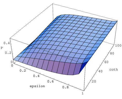
Figure 1: Dependence of tunneling probability P on the scaled dissipation $\epsilon={\lambda/\omega}$ and the temperature $T$ of the thermal bath, via $\coth({\hbar\omega/2kT}),$ for $\mu=0$ and for fixed values of the scaled initial position $z=-3,$ scaled initial momentum $v=-0.5$ and scaled inverse wave packet size $r=0.5.$

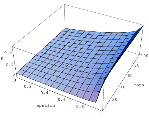
Figure 2: Same as in Fig. 1, but with $z=-3,$ $v=-0.5$ and $r=0.1.$

In the next four figures, we consider $\mu\neq 0.$ Figs. 3 and 4 show the dependence of the penetration probability on the scaled dissipation and on the parameter $\gamma$ for a fixed scaled initial position $z$, momentum $v$ and wave packet size $r$ at the temperature $T=0.$

Figure 3: Dependence of tunneling probability P on the scaled dissipation $\epsilon$ and parameter $\gamma=\mu/\omega,$ for the temperature $T=0$ of the thermal bath and for fixed values of the scaled initial position $z=-3,$ scaled initial momentum $v=-0.5$ and scaled inverse wave packet size $r=0.3.$

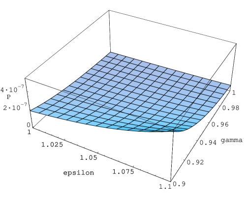
Figure 4: Same as in Fig. 3, but with $z=-9,$ $v=-0.9$ and $r=0.3.$

In Figs. 5 and 6 we give the dependence of the penetration probability on the scaled dissipation and temperature, at fixed values of $z,v,r$ and $\gamma.$ The presented dependence of the penetration probability on these variables can be summarized in the following conclusions:

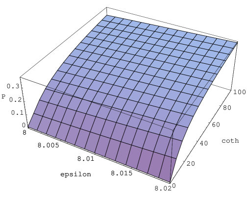
Figure 5: Dependence of tunneling probability P on the scaled dissipation $\epsilon$ and the temperature $T$ of the thermal bath, via $\coth({\hbar\omega/2kT}),$ for $\gamma=7.99$ and for fixed values of the scaled initial position $z=-3,$ scaled initial momentum $v=-0.5$ and scaled inverse wave packet size $r=0.5.$

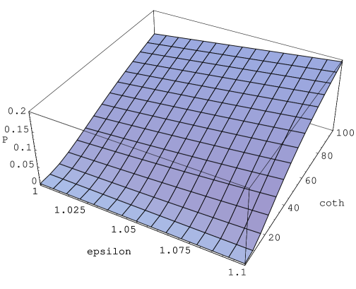
Figure 6: Same as in Fig. 5, but with $\gamma=0.97,$ $z=-9,$ $v=-0.9$ and $r=0.5.$

1) When the scaled initial momentum $|v|$ is increasing, then $P$ is increasing up to 1/2 if the particle does not have enough kinetic energy to pass the potential barrier. The same conclusion is valid for the variable $r,$ i. e. if the initial width of the Gaussian packet is decreasing, then the penetration probability is increasing.

2) If the scaled initial position $|z|$ is increasing, then $P$ is decreasing from 1/2 to 0 if the particle does not have enough kinetic energy to pass the potential barrier.

3) The penetration probability is increasing from 0 to 1/2 with dissipation and with $\coth(\hbar\omega/2kT)$ and, therefore, with the temperature. For the case $\mu\neq 0,$ the probability $P$ is decreasing with $\mu.$

In conclusion, the dependence of the tunneling probability on dissipation is not simple. When the particle does not have enough kinetic energy to pass the parabolic barrier, which is the relevant case to the quantum tunneling problem, the dissipation enhances tunneling.

5 Summary

In the framework of the Lindblad theory for open quantum systems, we have formulated the motion and the spreading of Gaussian wave packets in an inverted oscillator potential. We have obtained analytic solutions of evolution in time of the wave packets and of the barrier penetrability. Since the wave packets spread in time according to the same law of evolution as their center moves, the value of barrier penetrability is in general different from 1/2. The inverted oscillator potential has an important physical relevance, since it can constitute a guide how to treat more physically realistic potentials, like third order and double-well potentials [27, 33] or joined inverted parabola and harmonic oscillator potentials [34], in order to be applied in nuclear fission and in molecular or solid state physics.

Acknowledgments

One of us (A. I.) is pleased to express his sincere gratitude for the hospitality at the Institut für Theoretische Physik in Giessen. A. I. also gratefully acknowledges financial support by the DAAD (Germany).

References

- [1] A. O. Caldeira and A. J. Leggett, Phys. Rev. Lett. 46, 211 (1981)
- [2] A. O. Caldeira and A. J. Leggett, Ann. Phys. (N. Y.) 149, 374 (1983)
- [3] A. J. Bray and M. A. Moore, Phys. Rev. Lett. 49, 1545 (1982)
- [4] S. Chakravarty, Phys. Rev. Lett. 49, 681 (1982)
- [5] G. Schön and A. D. Zaikin, Phys. Rep. 198, 237 (1990)
- [6] S. Chakravarty and A. J. Leggett, Phys. Rev. Lett. 52, 5 (1984)
- [7] A. J. Leggett, S. Chakravarty, A. T. Dorsey, M. P. A. Fisher, A. Garg and W. Zweger, Rev. Mod. Phys. 59, 1 (1987)
- [8] U. Weiss, Quantum Dissipative Systems (World Scientific, Singapore, 1992)
- [9] H. Dekker, Phys. Rev. A 38, 6351 (1988)
- [10] G. W. Ford, J. T. Lewis and R. F. O’ Connell, Phys. Lett. A 158, 367 (1991)
- [11] M. Razavi and A. Pimpale, Phys. Rep. 168, 305 (1988)
- [12] H. Hofmann, Phys. Rep. 284, 137 (1997)
- [13] A. Schmid, Ann. Phys. (N. Y.) 170, 333 (1986)
- [14] A. Widom and T. D. Clark, Phys. Rev. Lett. 48, 63 (1982)
- [15] R. Bruinsma and P. Bak, Phys. Rev. Lett. 56, 420 (1986)
- [16] A. J. Leggett, Phys. Rev. B 30, 1208 (1984)
- [17] M. Razavy, Phys. Rev. A 41, 6668 (1990)
- [18] K. Fujikawa, S. Iso, M. Sasaki and H. Suzuki, Phys. Rev. Lett. 68, 1093 (1992)
- [19] E. G. Harris, Phys. Rev. A 48, 995 (1993)
- [20] L. H. Yu, Phys. Rev. A 54, 3779 (1996)
- [21] J. Ankerhold, H. Grabert and G. L. Ingold, Phys. Rev. E 51, 4267 (1995)
- [22] J. Ankerhold and H. Grabert, Phys. Rev. E 52, 4704 (1995); 55, 1355 (1997)
- [23] E. B. Davies, Quantum Theory of Open Systems (Academic Press, New York, 1976)
- [24] G. Lindblad, Commun. Math. Phys. 48, 119 (1976)
- [25] H. Spohn, Rev. Mod. Phys. 52, 569 (1980)
- [26] E. Stefanescu, A. Sandulescu and W. Greiner, Int. J. Mod. Phys. E 2, 233 (1993)
- [27] G. G. Adamian, N. V. Antonenko and W. Scheid, Phys. Lett. A 244, 482 (1998)
- [28] A. Isar, A. Sandulescu, H. Scutaru, E. Stefanescu and W. Scheid, Int. J. Mod. Phys. E 3, 635 (1994)
- [29] A. Sandulescu and H. Scutaru, Ann. Phys. (N. Y.) 173, 277 (1987)
- [30] A. Isar, Helv. Phys. Acta 67, 436 (1994)
- [31] A. Isar, W. Scheid and A. Sandulescu, J. Math. Phys. 32, 2128 (1991)
- [32] A. Isar, A. Sandulescu and W. Scheid, Int. J. Mod. Phys. B 10, 2767 (1996)
- [33] G. G. Adamian, N. V. Antonenko and W. Scheid, Nucl. Phys. A 645, 376 (1999)
- [34] S. Misicu, quant-ph/9906012