Scalable superconducting charge qubit quantum computer via gate voltage and external flux

Abstract

We present a scalable scheme for superconducting charge qubits with the assistance of one-dimensional superconducting transmission line resonator (STLR) playing the role of data bus. The coupling between qubit and data bus may be turned on and off by just controlling the gate voltage and externally applied flux of superconducting charge qubit. In our proposal, the entanglement between arbitrary two qubits and $W$ states of three qubits can be generated quickly and easily.

I introduction

As a candidate of scalable solid-state quantum computer, superconducting circuits with Josephson junction makhlin have attracted much attention in recent years. A series of successful experiments in single superconducting charge nakamura , flux mooij and phase yu qubits have demonstrated the macroscopic quantum coherence and the relative long coherence time. Due to the good performance of single superconducting qubit, people are now exploring the possibility for scaling up to many qubits.

Two-qubit experiments have been performed in superconducting charge pashkin ; yamamoto , flux izmalkov ; majer ; plourde and phase xu ; berkley ; mcdermott qubits and the entanglement has been observed. Usually, the interaction between qubits in these experiments is always on during the manipulation. There are many theoretical proposals makhlin ; shnirman ; you ; wang1 ; blais1 ; averin ; cosmelli for coupling any pair of qubits selectively through a common data bus or by adding additional sub-circuits. There are currently experimental efforts in implementing these proposals.

Recently, superconducting qubits coupled to an $LC$ oscillator or one-dimensional superconducting transmission line resonator (STLR) blais2 has attracted much interest. Such systems were of great interest not only in the study of the fundamental quantum mechanics of open systems but also as the potential candidates of scalable superconducting quantum computers. In the ion-trap quantum computer cirac , the harmonic oscillator played an important role as data bus. Similarly, the $LC$ oscillator or STLR can also play the role of data bus. Data-bus plays an important role in quantum information processing spiller . With the help of data bus, state transfer wang2 and $n$-qubit controlled phase gate yang for superconducting phase qubits were proposed. By coupling a charge qubit with a micro-cavity, macroscopic superposition states can be generated by manipulating the gate voltage and external flux in an elegant way in Refs. nori . By using the appropriate time-dependent electromagnetic fields, Liu et al. liu presented a scheme of scalable circuit for superconducting flux qubits, where quantum two-gate is realized by applying an external classical light fields.

The work of liu provides a scalable superconducting quantum computer scheme using flux qubit. Inspired by the interesting idea in Ref.liu , we present a scalable superconducting charge quantum computer scheme up to many qubits with the assistance of STLR playing the role of data bus. In this scheme, both single- and two- qubit gates can be implemented by just controlling the gate voltage and externally applied flux. It is found that Bell states and $W$ states can be generated quickly in a simple way.

II The model Hamiltonian

II.1 Single superconducting charge qubit

The single superconducting charge qubit consists of a small superconducting island with cooper-pair charge $Q=2ne$ connected by two identical Josephson junctions(each with capacitance $C_{J}$ and Josephson coupling energy $E_{J}$) to a superconducting electrode. This is the structure of a dc SQUID. A gate voltage $V_{g}$ is coupled to the superconducting island through gate capacitance $C_{g}$. The gate voltage $V_{g}$ and externally applied flux $\Phi_{e}$ are externally controlled and used to bias the superconducting island and the dc SQUID. A schematic diagram of the single-qubit structure is show in Fig.1. The Hamiltonian of the system is

$$H_{q}=E_{c}(n-n_{g})^{2}-2E_{J}\cos(\frac{\pi\Phi_{e}}{\Phi_{0}})\cos\varphi,$$ (1)

where

$$E_{c}=\frac{(2e)^{2}}{2(2C_{J}+C_{g})}$$ (2)

is the single-cooper-pair charging energy of the island, $n_{g}=C_{g}V_{g}/2e$ is the gate charge induced by the gate voltage, $-2E_{J}\cos(\pi\Phi_{e}/\Phi_{0})$ is the effective Josephson coupling energy and $\Phi_{0}=h/2e$ is the flux quantum.

Figure 1: The structure of superconducting charge qubit. The Josephson coupling energy and capacitance of the two identical Josephson junctions is $E_{J}$ and $C_{J}$. The gate voltage $V_{g}$ and externally applied flux $\Phi_{e}$ are used to bias the superconducting island and the dc SQUID.

In the charge regime, that is $E_{c}\gg E_{J}$, and in the neighborhood of $n_{g}=1/2$, only two charge states, say $|0\rangle$ and $|1\rangle$, are relevant. In the representation of this two charge states, the reduced two-state Hamiltonian can be written in the spin-$1/2$ form

$$H_{q}=-\frac{1}{2}E_{c}(1-2n_{g})\sigma_{z}-E_{J}\cos(\frac{\pi\Phi_{e}}{\Phi_{0}})\sigma_{x}.$$ (3)

The eigenvalues of single-qubit Hamiltonian are

$$E_{\pm}=\pm E=\pm\sqrt{\frac{1}{4}E_{c}^{2}(1-2n_{g})^{2}+E_{J}^{2}\cos^{2}(\frac{\pi\Phi_{e}}{\Phi_{0}})},$$

and eigenstates

$$|g\rangle=\sin\frac{\eta}{2}|1\rangle+\cos\frac{\eta}{2}|0\rangle,$$ (4)

$$|e\rangle=\cos\frac{\eta}{2}|1\rangle-\sin\frac{\eta}{2}|0\rangle,$$

where

$$\eta=\tan^{-1}(\frac{2E_{J}\cos(\frac{\pi\Phi_{e}}{\Phi_{0}})}{{E_{c}(1-2n_{g})}}).$$

In the representation of eigenbasis, the Hamiltonian is diagonalized as

$$H_{q}=-\frac{1}{2}\hbar\Omega\rho_{z},$$ (5)

where $\Omega=2E/\hbar$ and $\rho_{z}=|g\rangle\langle g|-|e\rangle\langle e|$.

II.2 Interaction of the charge qubit with one-dimensional cavity

Here we consider the one-dimensional cavity realized by STLR blais2 . For an ideal one-dimensional STLR with length $l$ and the boundary conditions $I(0,t)=I(l,t)=0$, the quantized current is

$$I=\sum_{k}\sqrt{\frac{\hbar\omega_{k}}{lL}}(a_{k}^{\dagger}+a_{k})\sin\frac{k\pi x}{l},$$

where $\omega_{k}=k\pi/(l\sqrt{LC})$ and $L$ $(C)$ is the inductance (capacitance) per unit length. The Hamiltonian of the STLR reads

$$H_{c}=\sum_{k}\hbar\omega_{k}(a_{k}a_{k}^{\dagger}+\frac{1}{2}).$$ (6)

Consider the $k$-th mode of the STLR, the current

$$I_{k}=\sqrt{\frac{\hbar\omega_{k}}{lL}}(a_{k}^{\dagger}+a_{k})\sin\frac{k\pi x}{l}.$$

Placing the superconducting qubits at the points $x=(2n+1)l/2k$, where $n$ is an arbitrary integer, the Hamiltonian of the combined system reads

$$H_{t} = \hbar\omega(a^{\dagger}a+\frac{1}{2})-\frac{1}{2}E_{c}(1-2n_{g})\sigma_{z}$$ (7)

$$-E_{J}\cos(\frac{\pi(\Phi_{e}+\Phi_{q})}{\Phi_{0}})\sigma_{x},$$

where $\Phi_{q}=\mu_{0}S\sqrt{\hbar\omega/lL}(a^{\dagger}+a)/(2\pi d)$ is the quantized magnetic flux induced by the quantized current, $d$ is the distance between the qubit and STLR and $S$ is the area enclosed by the dc SQUID. Here, for simplicity, we denote $\omega_{k}$ as $\omega$ and $a_{k}$ as $a$. Generally speaking, $\Phi_{q}\ll\Phi_{e}$, then the Hamiltonian(7) approximately reads

$$H_{t} = \hbar\omega(a^{\dagger}a+\frac{1}{2})-\frac{1}{2}E_{c}(1-2n_{g})\sigma_{z}-E_{J}\cos(\frac{\pi\Phi_{e}}{\Phi_{0}})\sigma_{x}$$

$$+\frac{\mu_{0}E_{J}S}{2\Phi_{0}d}\sqrt{\frac{\hbar\omega}{lL}}\sin(\frac{\pi\Phi_{e}}{\Phi_{0}})(a^{\dagger}+a)\sigma_{x}.$$

In the eigenbasis of the qubit’s Hamiltonian and under the rotating-wave approximation, the total Hamiltonian of the combined system (qubit and STLR) reads

$$H=\hbar\omega(a^{\dagger}a+\frac{1}{2})-\frac{1}{2}\hbar\Omega\rho_{z}+\hbar\lambda(a^{\dagger}\rho_{-}+\rho_{+}a),$$ (8)

where $\rho_{+}=|e\rangle\langle g|$, $\rho_{-}=|g\rangle\langle e|$ and the coupling coefficient of qubit and STLR

$$\lambda=\frac{\mu_{0}E_{J}S}{2\Phi_{0}d}\sqrt{\frac{\hbar\omega}{lL}}\sin(\frac{\pi\Phi_{e}}{\Phi_{0}})\cos\eta.$$

III Single qubit manipulation and two-qubit phase gate

Any unitary transformation can be constructed from a set of basic elementary gates. We adopt the scheme for single qubit manipulation in Ref.liu . However, different from the flux-qubit in Ref.liu , two-qubit gate in our scheme is realized by adjusting the gate voltage and the externally applied flux.

Single qubit manipulation can be easily implemented. In the Hamiltonian Eq.(8), which has been well studied in quantum optics walls , in the large detuning limit, that is $|\Delta|=|\Omega-\omega|\gg|\lambda|$, the interaction between qubit and STLR can be neglected sun . In this regime, the single qubit manipulation may be implemented by changing $n_{g}$ and $\Phi_{e}$ rapidly, as if the superconducting transmission line were absent. It has already been demonstrated in general in experiments nakamura ; pashkin ; yamamoto .

We now study the two-qubit gate. By controlling gate voltage and the externally applied flux, one can set a qubit resonating with the STLR, that is $\Delta=0$. In the resonant case, the evolutions of the states of qubit and STLR are

$$|g,0\rangle\rightarrow|g,0\rangle,$$ (9a)

$$|g,n+1\rangle\rightarrow$$

$$[\cos(\sqrt{n+1}\lambda t)|g,n+1\rangle-i\sin(\sqrt{n+1}\lambda t)|e,n\rangle],$$ (9b)

$$|e,n\rangle\rightarrow$$

$$[\cos(\sqrt{n+1}\lambda t)|e,n\rangle-i\sin(\sqrt{n+1}\lambda t)|g,n+1\rangle].$$ (9c)

Here, in Eq.(9b) and (9c) we dropped a global phase factor $e^{-i(n+1)\omega t}$.

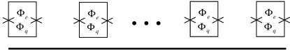
Figure 2: The N qubits are placed at the points $x=(2n+1)l/(2k)$ along the STLR, $n$ is an arbitrary integer. $\Phi_{e}$ and $\Phi_{q}$ are externally applied flux and flux induced by the transmission line.

A scalable quantum circuit can be constructed by placing $N$ charge qubits at the points $x=(2n+1)l/(2k)$ along the STLR acting as the data bus, as shown in Fig.2, and a similar setup where the qubits are connected by capacitances has been given in Ref. wangyd where phase transition has been studied in detail. The Hamiltonian of the system reads

$$H_{s}=\hbar\omega(a^{\dagger}a+\frac{1}{2})-\frac{1}{2}\hbar\sum_{k=1}^{N}\Omega_{k}\sigma_{z}^{(k)}+\hbar\sum_{k=1}^{N}\lambda_{k}(a^{\dagger}\rho_{-}^{(k)}+\rho_{+}^{(k)}a).$$ (10)

If the detuning between each qubit and STLR is great larger than their coupling constants, that is $|\lambda_{k}|/|\Delta_{k}|\ll 1$, then all N qubits are decoupled from the cavity, so one can do the single-qubit operations as discussed above.

To implement two-qubit manipulations, the selected two qubits should be sequentially coupled to the STLR. Suppose we want to implement a two-qubit manipulation acting on the $i$-th and $j$-th qubits, we can sequentially setting the the $i$-th and $j$-th resonating with the STLR. Firstly, we consider how to implement a two-qubit phase gate. Initially set the STLR in the vacuum state $|0\rangle$, and let the $i$-th qubit, the $j$-th qubit and then the $i$-th qubit sequentially resonating with the STLR for time duration $\tau_{1}$, $\tau_{2}$ and $\tau_{3}$ with $\tau_{1}=\tau_{2}=\tau_{3}=2\pi/\lambda$, according to formulas (9), the dynamical evolutions of the four states $|g_{i},g_{j},0\rangle$, $|g_{i},e_{j},0\rangle$, $|e_{i},g_{j},0\rangle$, $|e_{i},e_{j},0\rangle$ are

$$|g_{i},g_{j},0\rangle \rightarrow e^{i\theta_{1}}|g_{i},g_{j},0\rangle,$$ (11a)

$$|g_{i},e_{j},0\rangle \rightarrow e^{i\theta_{2}}|g_{i},e_{j},0\rangle,$$ (11b)

$$|e_{i},g_{j},0\rangle \rightarrow e^{i\theta_{3}}|e_{i},g_{j},0\rangle,$$ (11c)

$$|e_{i},e_{j},0\rangle \rightarrow e^{i\theta_{4}}|e_{i},e_{j},0\rangle$$ (11d)

with

$$\theta_{1} =\frac{(\Omega_{i}+2\Omega_{j})\pi}{\lambda},$$ (12a)

$$\theta_{2} =-\frac{(-\Omega_{i}+2\Omega_{j}+2\omega)\pi}{\lambda},$$ (12b)

$$\theta_{3} =-\frac{(\Omega_{i}-2\Omega_{j}+4\omega)\pi}{\lambda},$$ (12c)

$$\theta_{4} =-\frac{i(\Omega_{i}+2\Omega_{j}+6\omega)\pi}{\lambda}.$$ (12d)

Here, we assume that eigenfrequencies $\Omega_{i}$s of qubits are different when the qubits are not resonant with the STLR. In fact, the result won’t be affected even if the eigenfrequencies $\Omega_{i}$s are equal. After the dynamical evolutions with the given time durations, a two-qubit phase gate is constructed as follows

$$U_{p}=\left(\begin{array}[]{cccc}e^{i\theta_{1}}&0&0&0\\ 0&e^{-i\theta_{2}}&0&0\\ 0&0&e^{-i\theta_{3}}&0\\ 0&0&0&e^{-i\theta_{4}}\end{array}\right)$$ (17)

Because all of the two-qubit gates are universal deutsch , any two qubit operation can be obtained by combining the two-qubit phase gate $U_{p}$ with well-chosen single-qubit operations for the $i$-th and $j$-th qubits. Therefore, quantum computation can be realized by combination of two-qubit phase gate with single-qubit operations.

IV generation of entanglement

IV.1 two-qubit entanglement

The entangled state between the $i$-th and $j$-th qubits can be easily generated with the assistance of STLR. If two qubits, say the $i$-th and $j$-th qubits, resonate with the STLR simultaneously, the Hamiltonian of the system reads

$$H_{I}=\hbar\omega(a^{\dagger}a+\frac{1}{2})-\frac{1}{2}\hbar\sum_{k=i,j}\omega\sigma_{z}^{(k)}+\hbar\sum_{k=i,j}\lambda_{k}(a^{\dagger}\rho_{-}^{(k)}+\rho_{+}^{(k)}a),$$ (18)

here, for simplicity, we assumed that the coupling coefficient $\lambda_{k}$ is the same when qubits resonate with the STLR. The eigenvalues of Hamiltonian Eq.(18) are

$$E_{1}=\hbar\omega(n-\frac{1}{2})-\hbar\lambda\sqrt{4n-2},$$ (19a)

$$E_{2}=E_{3}=\hbar\omega(n-\frac{1}{2}),$$ (19b)

$$E_{4}=\hbar\omega(n-\frac{1}{2})+\hbar\lambda\sqrt{4n-2},$$ (19c)

and the corresponding eigenvectors are

$$|\psi_{1}\rangle = -\sqrt{\frac{n}{4n-2}}|g,g,n\rangle+\frac{1}{2}|g,e,n-1\rangle$$ (20a)

$$+\frac{1}{2}|e,g,n-1\rangle-\sqrt{\frac{n-1}{4n-2}}|e,e,n-2\rangle,$$

$$|\psi_{2}\rangle = -\sqrt{\frac{n-1}{2n-1}}|g,g,n\rangle+\sqrt{\frac{n}{2n-1}}|e,e,n-2\rangle,$$ (20b)

$$|\psi_{3}\rangle = -\frac{1}{\sqrt{2}}|g,e,n-1\rangle+\frac{1}{\sqrt{2}}|e,g,n-1\rangle,$$ (20c)

$$|\psi_{4}\rangle = \sqrt{\frac{n}{4n-2}}|g,g,n\rangle+\frac{1}{2}|g,e,n-1\rangle$$ (20d)

$$+\frac{1}{2}|e,g,n-1\rangle+\sqrt{\frac{n-1}{4n-2}}|e,e,n-2\rangle.$$

The ground state of Hamiltonian Eq.(18) is $|g,g,0\rangle$ and the corresponding energy is $E=-\frac{1}{2}\hbar\omega$. From the eigen-states, it is easy to write out the evolution of the system. For instance if the initial state of the system is $|g,g,1\rangle$, the state at time $t$ will be

$$|\psi(t)\rangle = e^{-\frac{i\omega t}{2}}[\cos(\sqrt{2}\lambda t)|g,g,1\rangle-\frac{i}{\sqrt{2}}\sin(\sqrt{2}\lambda t)|g,e,0\rangle$$ (21)

$$-\frac{i}{\sqrt{2}}\sin(\sqrt{2}\lambda t)|e,g,0\rangle].$$

When $\sqrt{2}\lambda t=\pi/2$, the state of the $i$-th and $j$-th qubits is a Bell-state becomes a Bell-state $|\Psi_{+}\rangle=(|g,e\rangle+|e,g\rangle)/{\sqrt{2}}$. Usually, the state of the STLR is in the vacuum state $|0\rangle$, to prepare the system in state $|g,g,1\rangle$, we first start from state $|e,g,0\rangle$, then setting $i$-th qubit resonating with STLR for a time duration $\tau_{1}=\pi/(2\lambda)$, and according to Eq. (9c), the state becomes $|g,g,1\rangle$. Then the Bell-state is obtained by setting $i$-th and $j$-th qubit resonating simultaneously with the STLR for a period of $\tau_{2}=\pi/(2\sqrt{2}\lambda)$, as shown in Eq. (21).

IV.2 Generation of $W$ states

In this section, we discuss the generation of $W$ states of arbitrary three qubits. Using sequential resonance between qubits and STLR, the $W$ states can be generated in a similar way to the generation of Bell states. We consider the $i$-th, $j$-th and $k$-th qubits. Suppose the initial states of the three qubits $i$, $j$, $k$ and STLR are $|g\rangle$, $|g\rangle$, $|e\rangle$ and vacuum state $|0\rangle$, respectively. Firstly, setting the $k$-th qubit resonating with STLR for a time duration $t_{1}$, according to Eq.(9), the evolution of state of the $k$-th qubit and STLR is

$$|e\rangle_{k}|0\rangle\rightarrow\cos(\lambda t_{1})|e\rangle_{k}|0\rangle-i\sin(\lambda t)|g\rangle_{k}|1\rangle,$$

here, we neglect a global phase factor $e^{-i\omega t_{1}}$. Secondly, setting the $i$-th and $j$-th qubit resonating with STLR for a time duration $t_{2}$, according to Eq.(20), the state of the combined system (three qubits and STLR) becomes

$$e^{\frac{i\omega t_{2}}{2}}\cos(\lambda t_{1})|g\rangle_{i}|g\rangle_{j}|e\rangle_{k}|0\rangle$$

$$-ie^{-\frac{i\omega t_{2}}{2}}\sin(\lambda t_{1})[\cos(\sqrt{2}\lambda t_{2})|g\rangle_{i}|g\rangle_{j}|g\rangle_{k}|1\rangle$$

$$-\frac{i}{\sqrt{2}}\sin(\sqrt{2}\lambda t_{2})|g\rangle_{i}|e\rangle_{j}|g\rangle_{k}|0\rangle$$

$$-\frac{i}{\sqrt{2}}\sin(\sqrt{2}\lambda t_{2})|e\rangle_{i}|g\rangle_{j}|g\rangle_{k}|0\rangle].$$ (22)

If the resonating time $t_{2}$ satisfies $\cos(\sqrt{2}\lambda t_{2})=\pi/2$, that is $t_{2}=\pi/(2\sqrt{2}\lambda)$, the state of the combined system reads

$$[\cos(\lambda t_{1})|g,g,e\rangle$$

$$-\frac{1}{\sqrt{2}}\sin(\lambda t_{1})e^{-i\frac{\omega\pi}{2\sqrt{2}\lambda}}(|g,e,g\rangle+|e,g,g\rangle)]|0\rangle,$$ (23)

where we neglect a global phase factor $e^{i\omega\pi/(4\sqrt{2}\lambda)}$ and the subscripts $i$, $j$, $k$. If the resonating time $t_{1}$ satisfies $\cos(\lambda t_{1})=\sqrt{3}/3$, we can get the $W$ state of the three qubits

$$\frac{1}{\sqrt{3}}[|g,g,e\rangle\mp e^{-i\frac{\omega\pi}{2\sqrt{2}\lambda}}(|g,e,g\rangle+|e,g,g\rangle)],$$ (24)

the signs $\mp$ depends on the value of $\sin(\lambda t_{1})$.

V discussion and conclusion

It’s notable that the coupling coefficient $\lambda$ is different in the single-qubit operation and two-qubit gate operation, because $\lambda$ is the function of $\sin(\pi\Phi_{e}/\Phi_{0})\cos\eta$; moreover, $\Phi_{e}$ and $\eta$ are external controlled and different between single-qubit operation and two-qubit gate operation. However, the single qubit operation will not be affected so long as the condition $|\lambda|/|\Delta|\ll 1$ is satisfied during the single-qubit operation, and $\lambda$ can be tuned to its maximum value when the two-qubit gate operation begins. In this paper, we consider the current coupling between the superconducting charge qubit and the STLR, however, the same result can be achieved by voltage coupling.

In conclusion, we have presented a scheme for scalable superconducting charge qubits with the assistance of STLR playing the role of data bus. The coupling between the selected qubit and the STLR can be turned on and off by just controlling the gate voltage and externally applied flux of the superconducting qubit. As a result, the single-qubit manipulation can be performed when the qubit decoupled with the STLR, and two-qubit gate can be implemented by setting two qubits sequentially resonating with the STLR. The entanglement state between arbitrary two qubits and $W$ state of arbitrary three qubits can be generated easily and quickly. The operation time in our scheme is much shorter than the decoherence time of superconducting charge qubits according to recent experiments nakamura ; wallraff . Different from the flux qubit gate case where two-qubit gate needs a TDEF, both single- and two- qubit gates are implemented by changing the gate voltage and the external flux in our scheme, the same set of devices can be used for both of them, which is appealing to experiment.

- (1) Y. Makhlin, G. Schön, and A. Shnirman, Rev. Mod. Phys. 73, 357 (2001).
- (2) Y. Nakamura, Y. A. Pashkin and J. S. Tsai, Nature 398, 786 (1999).
- (3) J. E . Mooij, T. P. Orlando, L. Levitov, Lin Tian, C. H. van der Wal and S. Lloyd, Science 285, 1036 (1999).
- (4) Y. Yu, S. Han, X. Chu, S.-I. Chu and Z. Wang, Science 296, 889 (2002).
- (5) Y. A. Pashkin, T. Yamamoto, O. Astafiev, Y. Nakamura, D. V. Averin, and J. S. Tsai, Nature 421, 823 (2003).
- (6) T. Yamamoto, Y. A. Pashkin, O. Astafiev, Y. Nakamura, and J. S. Tsai, Nature 425, 941 (2003).
- (7) A. Izmalkov, M. Grajcar, E. Il’ichev, Th.Wagner, H.-G. Meyer, A.Yu. Smirnov, M. H. S. Amin, A. Maassen vanden Brink, and A.M. Zagoskin, Phys. Rev. Lett. 93, 037003 (2004).
- (8) J. B. Majer, F. G. Paauw, A. C. J. terHaar, C. J. P. M. Harmans and J. E. Mooij, Phys. Rev. Lett. 94, 090501 (2005).
- (9) B. L. T. Plourde, T. L. Robertson, P. A. Reichardt, T. Hime, S. Linzen, C.E. Wu, and J. Clarke, Phys. Rev. B 72, 060506(R) (2005).
- (10) H. Xu, F. W. Strauch, S. K. Dutta, P. R. Johnson, R. C. Ramos, A. J. Berkley, H. Paik, J. R. Anderson, A. J. Dragt, C. J. Lobb, and F. C. Wellstood, Phys. Rev. Lett. 94, 027003 (2005).
- (11) A. J. Berkley, H. Xu, R. C. Ramos, M. A. Gubrud, F. W. Strauch, R. R. Johnson, J. R. Anderson, A. J. Dragt, C. J. Lobb, and F. C. Wellstood, Science 300, 1548 (2003).
- (12) R. McDermott, R. W. Simmonds, M. Steffen, K. B. Cooper, K. Cicak, K. d. Osborn, S. Oh, D. P. Pappas, and J. M. Martinis, Science 307, 1299 (2005).
- (13) A. Shnirman, G. Schön, and Z. Hermon, Phys. Rev. Lett. 79, 2371 (1997).
- (14) J. Q. You, J. S. Tsai, and F. Nori, Phys. Rev. Lett. 89, 197902 (2002).
- (15) Y. D. Wang, P. Zhang, D. L. Zhou, and C. P. Sun, Phys, Rev. B 70, 224515 (2004).
- (16) A. Blais, A. Maassen van den Brink and A. M. Zagoskin, Phys. Rev. Lett. 90, 127901 (2003).
- (17) D. V. Averin, C. Bruder, Phys. Rev. Lett. 91, 057003 (2003).
- (18) C. Cosmelli, M. G. Castellano, F. Chiarello, R. Leoni, G. Torrioli, and P. Carelli, ArXiv: cond-matt/0403690.
- (19) A. Blais, R.-S. Huang, A. Wallraff, S. M. Girvin, and R. J. Schoelkopf, Phys. Rev. A 69, 062320 (2004).
- (20) J. I. Cirac, P. Zoller, Phys. Rev. Lett. 74, 4091 (1995).
- (21) Y. D. Wang, Z. D. Wang, and C. P. Sun, Phys. Rev. B 72, 172507 (2005).
- (22) T. P. Spiller, K. Nemoto, S. L. Braunstein, W. J. Munro, P. van Loock and G. J. Milburn, New J. Phys. 8, 30 (2006).
- (23) C.-P. Yang, S. Han, Phys. Rev. A 72, 032311 (2005).
- (24) Yu-xi Liu, L. F. Wei, and F. Nori, Rev. A 72, 033818 (2005); ibid, A 71, 063820 (2005).
- (25) Y. X. Liu, C. P. Sun, and F. Nori, Phys. Rev. A 74, 052321 (2006).
- (26) Y. D. Wang et al, ArXiv:quant-ph/0603014.
- (27) D. F. Walls, G. J. Milburn, Quantum Optics, Springer-verlag, Berlin, 1994.
- (28) C. P. Sun, L. F. Wei, Y. X. Liu, and F. Nori, Phys. Rev. A 73, 022318 (2006).
- (29) D. Deutsch, A. Barenco, and A. Ekert, Proc. R. Soc. London A 449, 669-670 (1995).
- (30) A. Wallraff, D. I. Schuster, A. Blais, L. Frunzio, R.- S. Huang, J. Majer, S. Kumar, S. M. Girvin, and R. J. Schoelkopf, Nature 431, 162 (2004).