Vector Cooper Pairs and Coherent-Population-Trapping-like States in Ensemble of Interacting Fermions

Abstract

Using the standard Hamiltonian of the BCS theory, we show that in an ensemble of interacting fermions with the spin 1/2 there exist coherent states $|NC\rangle$, which nullify the Hamiltonian of the interparticle interaction (scattering). These states have an analogy with the well-known in quantum optics the coherent population trapping (CPT) effect. The structure of these CPT-like states corresponds to Cooper pairs with the total spin $S$=1. The found states have a huge degree of degeneracy and carry a macroscopic magnetic moment, that allows us to construct a new model of the magnetism connected with the delocalized electrons in metals (conductors). A principal possibility to apply the obtained results to the superfluid ³He is also demonstrated.

I Introduction

The effect of coherent population trapping (CPT) (see Alz ; Ar1 ; Gr ; Agap ; Ar2 and references therein) is one of nonlinear interference effects. Owing to number of its manifestations in different optical phenomena and its practical applications CPT occupies one of leading place in modern laser physics, nonlinear and quantum optics. For example, CPT is used in high-resolution spectroscopy Hemmer ; Akulshin ; Scully_1 ; Kitching , nonlinear optics of resonance media Harris ; Kochar ; Scully_2 , laser cooling Aspect1 ; Aspect2 , atom optics and interferometry Marte ; Weitz ; Featonby , physics of quantum information mazets96 ; Fleschauer1 ; Fleschauer2 ; Liu ; Phillips ; Zibrov ; Wal .

In the case of classical resonant field the CPT theory has been developed for a three-state model Ar2 ; Gr as well as for multi-level systems with account for the level degeneracy Hioe ; sm ; Tumaikin ; Taichenachev1 ; Taichenachev2 . Recently we generalize this theory to the case of an ensemble of atoms interacting with a quantized light field Taich ; Taich2 . Note also the presence of BCS-type states under the CPT conditions Bolkart .

From the very general point of view the essence of CPT can be formulated as follows. Consider two quantum systems (particles or fields) $A$ and $B$. The interaction between them is described by the Hamiltonian $\widehat{V}_{A-B}$. Then the CPT effect occurs when there exists a non-trivial state $|NC\rangle$, which nullifies the interaction:

$$\widehat{V}_{A-B}|NC\rangle=0\,.$$ (1)

In this state, obviously, the energy exchange between the systems $A$ and $B$ is absent. However, information correlations of the systems can be very strong, leading to important physical consequences. Note that if the system $A$ is equivalent to the system $B$, then the condition (1) means the absence of the field self-interaction or of the interparticle interaction

$$\widehat{V}_{A-A}|NC\rangle=0\,.$$ (2)

From this general viewpoint the standard CPT effect in the resonant interaction of atoms with electromagnetic field is deciphered as follows: $A$ and $B$ are ensembles of atoms and resonant photons, respectively; $\widehat{V}_{A-B}=-(\hat{\bf d}{\bf E})$ is the dipole interaction operator, and $|NC\rangle$ is the dark state $|dark\rangle$:

$$-(\hat{\bf d}{\bf E})|dark\rangle=0\,,$$ (3)

In the course of the interaction atoms are accumulated in the dark state, after that they do not scatter light, and they are not scattered by light. The information on various parameters of the resonant field has been encoded in the state $|dark\rangle$ sm ; Taich ; Taich2 .

Our standpoint consists in the following. The CPT principle, expressed by (1) or (2), is sufficiently universal and it can manifest in various branches of physics. The significant progress in laser physics, spectroscopy, quantum and nonlinear optics caused by the invention of the CPT effect earnestly argues that such states should not be considered a priori as a mathematical artefact, despite their uncommonness and superficial paradoxicality. Thus, attempts to introduce CPT-like states (when they are present, of course) into a description of various phenomena from different branches of physics do not contradict to the general physical principles and they are well founded.

For the first time such a generalized approach to CPT has been developed in our early paper Tum , where it is pointed out that from a phenomenological viewpoint the CPT effect has a some likeness to the superconductivity. In Tum the following comparison is carried out: atoms and electromagnetic field from one side, electrons and phonons form the other side. Indeed, a gas of atoms being in the dark state $|dark\rangle$ do not interact with photons (see eq.(3)), similarly to electrons in a superconducting state in solids, which are not scattered by the phonon oscillations of a lattice. In the paper Tum a hypothesis on the possibility of an alternative (to the standard BCS theory Bar ) mechanism of superconductivity has been proposed. Namely, a quantum system of electrons and phonons coupled by the interaction Hamiltonian $\widehat{V}_{e-phonon}$ was considered. According to Tum , the new mechanism of superconductivity could be based on the existence of such a state $|NC\rangle$, which nullifies the interaction operator $\widehat{V}_{e-phonon}$:

$$\widehat{V}_{e-phonon}|NC\rangle=0\,,$$ (4)

analogously to eq.(3). However, an explicit form of the state $|NC\rangle$ was not found in Tum .

In the present paper for the standard Hamiltonian of interparticle interaction in the BCS model Bar we find in explicit and analytical form CPT-like states of the type (2). In contrast to the scalar Cooper pairs ($S$=$\,0$) in the standard BCS theory such CPT-like states are formed by pairs with the spin $S$=1, i.e. here a vector $p$-pairing takes place. However, these states have a huge degree of degeneracy and due to this reason they can not be used as a basis for new mechanism of the superconductivity as it has been suggested in our previous papers Tum ; TY . Nevertheless, the existence of such CPT-like states can lead to serious consequences, because these states carry a macroscopic magnetic moment, that allows a principal possibility to describe a new approach to the magnetism connected with the delocalized electrons in metals (conductors). Apart from these, the obtained results can be related to the description of the superfluid phase of ³He, which, as is known, appears due to the formation of Cooper pairs with the spin $S$=1.

II Ensemble of fermions in a finite volume

Consider an ensemble of ${\cal N}$ fermions confined to a volume $V$, where ${\cal N}$=$n$$V$, and $n$ is the density of particles. We will use the standard BCS Hamiltonian Bar :

$$\widehat{H}_{BCS}=\widehat{H}_{0}+\widehat{W}\,.$$ (5)

The Hamiltonian of free particles can be written as:

$$\widehat{H}_{0}=\sum_{s,{\bf k}}\varepsilon_{\bf k}\,\hat{a}^{{\dagger}}_{s{\bf k}}\hat{a}_{s{\bf k}}\,,$$ (6)

where $\hat{a}^{{\dagger}}_{s{\bf k}}$($\hat{a}_{s{\bf k}}$) is the creation (annihilation) operator of Fermi particle in the state with wavevector ${\bf k}$ and spin projection $s=\uparrow,\downarrow$, and $\varepsilon_{k}$ is the energy of this state. These operators satisfy the following anticommutator relationships:

$$\hat{a}^{{\dagger}}_{s{\bf k}}\hat{a}_{s^{\prime}{\bf k^{\prime}}}+\hat{a}_{s^{\prime}{\bf k^{\prime}}}\hat{a}^{{\dagger}}_{s{\bf k}}=\delta_{ss^{\prime}}\delta_{\bf kk^{\prime}},$$

$$\hat{a}_{s{\bf k}}\hat{a}_{s^{\prime}{\bf k^{\prime}}}+\hat{a}_{s^{\prime}{\bf k^{\prime}}}\hat{a}_{s{\bf k}}=0,$$

$$\hat{a}^{{\dagger}}_{s{\bf k}}\hat{a}^{{\dagger}}_{s^{\prime}{\bf k^{\prime}}}+\hat{a}^{{\dagger}}_{s^{\prime}{\bf k^{\prime}}}\hat{a}^{{\dagger}}_{s{\bf k}}=0\,.$$ (7)

The interaction between particles is described by the Hamiltonian coupling particles with opposite momenta and spin:

$$\widehat{W}=\frac{g}{V}\sum_{{\bf k}_{1,2}\in{\cal D}_{F}}G({\bf k}_{1},{\bf k}_{2})\,\hat{a}^{{\dagger}}_{\uparrow{\bf k}_{1}}\hat{a}^{{\dagger}}_{\downarrow-{\bf k}_{1}}\hat{a}_{\downarrow-{\bf k}_{2}}\hat{a}_{\uparrow{\bf k}_{2}}\,,$$ (8)

$${\cal D}_{F}:\;\;k_{F}-\Delta\leq|{\bf k}|\leq k_{F}+\Delta\,.$$

Only particles with wavevectors in the thin layer of the width $2\Delta$ around the Fermi surface (see in Fig.1a), having the radius $k_{F}$ ($\Delta$$\ll$$\,k_{F}$), are involved in the interaction. This subset in the wavevector space will be referred to as ${\cal D}_{F}$. If even one of the vectors ${\bf k}_{1,2}$ does not belong to the subset ${\cal D}_{F}$, then $G$(${\bf k}_{1},$${\bf k}_{2}$)=0. The sign of the interaction constant $g$ in (8) governs the attraction ($g$$<$0) or repulsion ($g$$>$0) between particles. The formfactor $G$(${\bf k}_{1},$${\bf k}_{2}$) obeys to the general symmetry condition

$$G({\bf k}_{1},{\bf k}_{2})=G(-{\bf k}_{1},{\bf k}_{2})=G({\bf k}_{1},-{\bf k}_{2})\,.$$ (9)

In this case the Hamiltonian $\widehat{W}$ consists of the quadratic operator constructions:

$$\hat{a}^{{\dagger}}_{\uparrow{\bf k}}\hat{a}^{{\dagger}}_{\downarrow-{\bf k}}+\hat{a}^{{\dagger}}_{\uparrow-{\bf k}}\hat{a}^{{\dagger}}_{\downarrow{\bf k}}=\hat{a}^{{\dagger}}_{\uparrow{\bf k}}\hat{a}^{{\dagger}}_{\downarrow-{\bf k}}-\hat{a}^{{\dagger}}_{\downarrow{\bf k}}\hat{a}^{{\dagger}}_{\uparrow-{\bf k}}\,,$$

$$\hat{a}_{\uparrow{\bf k}}\hat{a}_{\downarrow-{\bf k}}+\hat{a}_{\uparrow-{\bf k}}\hat{a}_{\downarrow{\bf k}}=\hat{a}_{\uparrow{\bf k}}\hat{a}_{\downarrow-{\bf k}}-\hat{a}_{\downarrow{\bf k}}\hat{a}_{\uparrow-{\bf k}}\,,$$ (10)

which are antisymmetrical with respect to the spin variables ($\uparrow$,$\downarrow$) and, consequently, they are scalar constructions. Thus, the operator $\widehat{W}$ has the invariant form (8) independently of the direction of the quantization axis $z$, with respect to which the spin projections ($\uparrow$,$\downarrow$) are determined. Thus, the relationship (9) is the consequence of the invariance of the Hamiltonian (8) with respect to the choice of the quantization axis $z$. It is usually assumed that $G$(${\bf k}_{1},$${\bf k}_{2}$)=1 at ${\bf k}_{1,2}$$\in$${\cal D}_{F}$.

Recall, that, according to the standard conceptions of the description of the conductivity electrons in metals, the model Hamiltonian (8) is governed by the interaction of electrons with phonons of lattice and Coulomb repulsion between electrons.

It should be especially noted that since the interaction Hamiltonian (8) consists of the scalar (with respect to the spin) constructions (II), then it was widely recognized that the standard mathematical BCS model describes only the scalar pairing of fermions. However, as it will be shown below, in the general case it is not so, i.e. the Hamiltonian (8) can describe the vector pairing as well.

Figure 1: Illustrations: a) thin spherical layer ${\cal D}_{F}$ with the width 2$\Delta$ around the Fermi surface with the radius $k_{F}$; b) upper hemispherical layer ${\cal D}_{F}^{(+)}$ with $k_{z}$$>$0.

III CPT-like states

It turns out that the operator (8) allows the existence of the CPT-like states $|NC\rangle$, obeying the condition

$$\widehat{W}|NC\rangle=0\,.$$ (11)

Let us build up these states. Consider first the following operator construction:

$$\hat{b}^{{\dagger}}_{\bf k}(\xi)=(\hat{a}^{{\dagger}}_{\uparrow{\bf k}}\hat{a}^{{\dagger}}_{\downarrow-{\bf k}}+\xi\,\hat{a}^{{\dagger}}_{\uparrow-{\bf k}}\hat{a}^{{\dagger}}_{\downarrow{\bf k}})/\sqrt{2}\,,$$ (12)

which generates two-particle coupled states with opposite wavevectors ${\bf k}$ and $-{\bf k}$, and with the zero projection of the total spin; the parameter $\xi$ is arbitrary number. Using the standard anticommutator rules for fermionic operators $\hat{a}^{{\dagger}}_{s{\bf k}}$ and $\hat{a}_{s{\bf k}}$, and the property (9), we calculate the commutator:

$$\left[\widehat{W},\,\hat{b}^{{\dagger}}_{\bf k}(\xi)\right]=\frac{g}{V\sqrt{2}}\sum_{{\bf k}_{1}\in{\cal D}_{F}}G({\bf k}_{1},{\bf k})\,\hat{a}^{{\dagger}}_{\uparrow{\bf k}_{1}}\hat{a}^{{\dagger}}_{\downarrow-{\bf k}_{1}}$$ (13)

$$(1+\xi-\xi\hat{a}^{{\dagger}}_{\uparrow-{\bf k}}\hat{a}_{\uparrow-{\bf k}}-\xi\hat{a}^{{\dagger}}_{\downarrow{\bf k}}\hat{a}_{\downarrow{\bf k}}-\hat{a}^{{\dagger}}_{\uparrow{\bf k}}\hat{a}_{\uparrow{\bf k}}-\hat{a}^{{\dagger}}_{\downarrow-{\bf k}}\hat{a}_{\downarrow-{\bf k}}).$$

As is seen, when $\xi=-1$ this commutator has the specific form, where all summands are finished by the annihilation operators $\hat{a}_{\uparrow\pm{\bf k}}$ and $\hat{a}_{\downarrow\pm{\bf k}}$. Therefore we define now the basic operator construction $\hat{\gamma}^{{\dagger}}_{0,\bf k}$:

$$\hat{\gamma}^{{\dagger}}_{0,\bf k}\equiv\hat{b}^{{\dagger}}_{\bf k}(-1)=(\hat{a}^{{\dagger}}_{\uparrow{\bf k}}\hat{a}^{{\dagger}}_{\downarrow-{\bf k}}-\hat{a}^{{\dagger}}_{\uparrow-{\bf k}}\hat{a}^{{\dagger}}_{\downarrow{\bf k}})/\sqrt{2}=$$

$$(\hat{a}^{{\dagger}}_{\uparrow{\bf k}}\hat{a}^{{\dagger}}_{\downarrow-{\bf k}}+\hat{a}^{{\dagger}}_{\downarrow{\bf k}}\hat{a}^{{\dagger}}_{\uparrow-{\bf k}})/\sqrt{2}\,,$$ (14)

which is symmetric on the spin variables $\uparrow$,$\downarrow$. For this construction the commutator (13) takes the form:

$$\left[\widehat{W},\,\hat{\gamma}^{{\dagger}}_{0,\bf k}\right]=\frac{g}{V\sqrt{2}}\sum_{{\bf k}_{1}\in{\cal D}_{F}}G({\bf k}_{1},{\bf k})\,\hat{a}^{{\dagger}}_{\uparrow{\bf k}_{1}}\hat{a}^{{\dagger}}_{\downarrow-{\bf k}_{1}}$$

$$(\hat{a}^{{\dagger}}_{\uparrow-{\bf k}}\hat{a}_{\uparrow-{\bf k}}+\hat{a}^{{\dagger}}_{\downarrow{\bf k}}\hat{a}_{\downarrow{\bf k}}-\hat{a}^{{\dagger}}_{\uparrow{\bf k}}\hat{a}_{\uparrow{\bf k}}-\hat{a}^{{\dagger}}_{\downarrow-{\bf k}}\hat{a}_{\downarrow-{\bf k}})\,.$$ (15)

Apart from the operator $\hat{\gamma}^{{\dagger}}_{0,\bf k}$ there exist the other two quadratic in the operators $\hat{a}^{{\dagger}}_{s\pm{\bf k}}$ constructions with the zero total momentum, for which the commutator with the operator $\widehat{W}$ is finished from the right side by the annihilation operators $\hat{a}_{s\pm{\bf k}}$. These construction are:

$$\hat{\gamma}^{{\dagger}}_{+1,\bf k}=\hat{a}^{{\dagger}}_{\uparrow{\bf k}}\hat{a}^{{\dagger}}_{\uparrow-{\bf k}}\,,\quad\hat{\gamma}^{{\dagger}}_{-1,\bf k}=\hat{a}^{{\dagger}}_{\downarrow{\bf k}}\hat{a}^{{\dagger}}_{\downarrow-{\bf k}}\,,$$ (16)

for them the following commutator relations are fulfilled:

$$\left[\widehat{W},\,\hat{\gamma}^{{\dagger}}_{+1,\bf k}\right]= \frac{g}{V}\sum_{{\bf k}_{1}\in{\cal D}_{F}}G({\bf k}_{1},{\bf k})\,\hat{a}^{{\dagger}}_{\uparrow{\bf k}_{1}}\hat{a}^{{\dagger}}_{\downarrow-{\bf k}_{1}}$$ (17)

$$(-\hat{a}^{{\dagger}}_{\uparrow-{\bf k}}\hat{a}_{\downarrow-{\bf k}}+\hat{a}^{{\dagger}}_{\uparrow{\bf k}}\hat{a}_{\downarrow{\bf k}})\,,$$

$$\left[\widehat{W},\,\hat{\gamma}^{{\dagger}}_{-1,\bf k}\right]= \frac{g}{V}\sum_{{\bf k}_{1}\in{\cal D}_{F}}G({\bf k}_{1},{\bf k})\,\hat{a}^{{\dagger}}_{\uparrow{\bf k}_{1}}\hat{a}^{{\dagger}}_{\downarrow-{\bf k}_{1}}$$ (18)

$$(\hat{a}^{{\dagger}}_{\downarrow-{\bf k}}\hat{a}_{\uparrow-{\bf k}}-\hat{a}^{{\dagger}}_{\downarrow{\bf k}}\hat{a}_{\uparrow{\bf k}})\,.$$

The expressions (III), (17), and (18) are crucial for the building up the CPT-like states (11).

A set of the three operators $\hat{\gamma}^{{\dagger}}_{q,\bf k}$ ($q$=0,$\pm 1$) for the given ${\bf k}$ constitutes an invariant (with respect to the choice of the quantization axis $z$) subspace and it describes the three orthogonal components of the particle spin $S$=1 (i.e. it corresponds to the vector particle). These components correspond to the spin projections (0,$\pm\hbar$) onto the $z$ axis. Thus, here we deal with the vector pairing of $p$-type, contrary to the scalar pairing of $s$-type ($S$=0).

Due to the obvious relationship

$$\hat{\gamma}^{{\dagger}}_{q,-\bf k}=-\hat{\gamma}^{{\dagger}}_{q,\bf k}\,,\quad(q=0,\pm 1)$$ (19)

the operators $\hat{\gamma}^{{\dagger}}_{q,\bf k}$, defined on the spherical layer ${\bf k}$$\in$${\cal D}_{F}$, are not independent. Therefore instead of the ${\cal D}_{F}$ we define a hemispherical layer in the wavevector space. For example, choose the upper hemispherical layer ${\cal D}_{F}^{(+)}$ (see Fig.1b), consisting of vectors ${\bf k}$$\in$${\cal D}_{F}$ with positive projections on the axis $z$ ($k_{z}$$>$$\,0$) only. Now the operators $\hat{\gamma}^{{\dagger}}_{q,\bf k}$, defined for vectors ${\bf k}$$\in$${\cal D}_{F}^{(+)}$ are independent. Note, that the introduction of the hemispherical layer in the wavevector space plays an auxiliary role, reducing some notations. The concrete choice of the hemispherical layer do not effect on the following results.

Let us demonstrate the method of the construction of the CPT-like states (11) using a concrete example. Consider the operator construction of the following form

$$\widehat{\Psi}_{NC}(...\hat{\gamma}^{{\dagger}}_{0,\bf k}...)=\prod_{{\bf k}\in{\cal D}_{F}^{(+)}}\hat{\gamma}^{{\dagger}}_{0,\bf k}\,,$$ (20)

consisting only of the operators $\hat{\gamma}^{{\dagger}}_{0,\bf k}$, which correspond to the zero spin projections of the vector particles (III). This construction acts on the upper hemispherical layer ${\cal D}_{F}^{(+)}$ (for each ${\bf k}$ the operator $\hat{\gamma}^{{\dagger}}_{0,\bf k}$ is used, at most, once). Obviously, the order of multipliers can be arbitrary, because [$\hat{\gamma}^{{\dagger}}_{q,\bf k}$$,\,$$\hat{\gamma}^{{\dagger}}_{q^{\prime},\bf k^{\prime}}$]=0. Let us factor out arbitrary operator $\hat{\gamma}^{{\dagger}}_{0,\bf k^{\prime}}$ in (20) from the product $\Pi$ and then act by the operator $\widehat{W}$ on $\widehat{\Psi}_{NC}(...\hat{\gamma}^{{\dagger}}_{0,\bf k}...)$:

$$\widehat{W}\widehat{\Psi}_{NC}(...\hat{\gamma}^{{\dagger}}_{0,\bf k}...)=\widehat{W}\hat{\gamma}^{{\dagger}}_{0,\bf k^{\prime}}\prod_{{\bf k}\neq{\bf k^{\prime}}}\hat{\gamma}^{{\dagger}}_{0,\bf k}=$$ (21)

$$\left(\hat{\gamma}^{{\dagger}}_{0,\bf k^{\prime}}\widehat{W}+[\widehat{W},\,\hat{\gamma}^{{\dagger}}_{0,\bf k^{\prime}}]\right)\prod_{{\bf k}\neq{\bf k^{\prime}}}\hat{\gamma}^{{\dagger}}_{0,\bf k}.$$

Since under the sign $\Pi$ in (21) the creation operators with wavevectors $\pm{\bf k^{\prime}}$ are absent, then, as is follows from eq.(III), the commutator $[\widehat{W},\,\hat{\gamma}^{{\dagger}}_{0,\bf k^{\prime}}]$ can be moved to the right side through the product $\Pi$. As a result, the expression (21) can be written as:

$$\widehat{W}\widehat{\Psi}_{NC}(...\hat{\gamma}^{{\dagger}}_{0,\bf k}...)=$$

$$\hat{\gamma}^{{\dagger}}_{0,\bf k^{\prime}}\widehat{W}\prod_{{\bf k}\neq{\bf k^{\prime}}}\hat{\gamma}^{{\dagger}}_{0,\bf k}+\left(\prod_{{\bf k}\neq{\bf k^{\prime}}}\hat{\gamma}^{{\dagger}}_{\bf k}\right)[\widehat{W},\,\hat{\gamma}^{{\dagger}}_{0,\bf k^{\prime}}]\,.$$ (22)

Let us consider also the operator construction

$$\widehat{\Phi}(\Delta)=\prod_{|{\bf k}|<(k_{F}-\Delta)}\hat{a}^{{\dagger}}_{\uparrow{\bf k}}\hat{a}^{{\dagger}}_{\downarrow{\bf k}}\,,$$ (23)

which, acting on the vacuum $|0\rangle$, generates the state, corresponding to the completely occupied sphere with the radius ($k_{F}-\Delta$) in the wavevector space (in Fig.1a it corresponds to the inner sphere shaded by skew lines). The following commutator relationships are evident:

$$[\widehat{W},\,\widehat{\Phi}(\Delta)]=0;\quad\left[[\widehat{W},\,\hat{\gamma}^{{\dagger}}_{q,\bf k}],\,\widehat{\Phi}(\Delta)\right]=0\quad({\bf k}\in{\cal D}_{F})\,,$$ (24)

because in the operator $\widehat{\Phi}(\Delta)$ (see (23)) only the wavevectors $|{\bf k}|$$<$$(k_{F}$$-\Delta)$ are used. These vectors do not belong to the upper layer ${\cal D}_{F}$ where the operators $\widehat{W}$ and $\hat{\gamma}^{{\dagger}}_{q,\bf k^{\prime}}$ act.

Let us prove that the state $|NC,...\hat{\gamma}^{{\dagger}}_{0,\bf k}...\rangle$, nullifying the interaction (11), has the form

$$|NC,...\hat{\gamma}^{{\dagger}}_{0,\bf k}...\rangle=\widehat{\Psi}_{NC}(...\hat{\gamma}^{{\dagger}}_{0,\bf k}...)\widehat{\Phi}(\Delta)|0\rangle\,.$$ (25)

Acting on this state by the operator $\widehat{W}$, and taking into account the relationships (III) and (24), one can obtain:

$$\widehat{W}\widehat{\Psi}_{NC}(...\hat{\gamma}^{{\dagger}}_{0,\bf k}...)\widehat{\Phi}(\Delta)|0\rangle=\hat{\gamma}^{{\dagger}}_{\bf k^{\prime}}\widehat{W}\left(\prod_{{\bf k}\neq{\bf k^{\prime}}}\hat{\gamma}^{{\dagger}}_{0,\bf k}\right)\widehat{\Phi}(\Delta)|0\rangle$$

$$+\left(\prod_{{\bf k}\neq{\bf k^{\prime}}}\hat{\gamma}^{{\dagger}}_{\bf k}\right)\widehat{\Phi}(\Delta)\,[\widehat{W},\,\hat{\gamma}^{{\dagger}}_{0,\bf k^{\prime}}]\,|0\rangle\,.$$ (26)

However, since the commutator (III) is finished from the right side by the annihilation operators, then [$\widehat{W}$$,\,$$\hat{\gamma}^{{\dagger}}_{0,\bf k^{\prime}}$]$|0\rangle=0$. Thus, from (III) we have

$$\widehat{W}\widehat{\Psi}_{NC}(...\hat{\gamma}^{{\dagger}}_{0,\bf k}...)\widehat{\Phi}(\Delta)|0\rangle=$$

$$\hat{\gamma}^{{\dagger}}_{0,\bf k^{\prime}}\widehat{W}\left(\prod_{{\bf k}\neq{\bf k^{\prime}}}\hat{\gamma}^{{\dagger}}_{0,\bf k}\right)\widehat{\Phi}(\Delta)|0\rangle\,,$$ (27)

From this equation we see that it is possible to change the order of the sequence of $\widehat{W}$ and any operator $\hat{\gamma}^{{\dagger}}_{0,\bf k}$. Proceeding this consideration step by step and taking into account (24), we obtain:

$$\widehat{W}|NC,...\hat{\gamma}^{{\dagger}}_{0,\bf k}...\rangle\equiv\widehat{W}\widehat{\Psi}_{NC}(...\hat{\gamma}^{{\dagger}}_{0,\bf k}...)\widehat{\Phi}(\Delta)|0\rangle=$$

$$\widehat{\Psi}_{NC}(...\hat{\gamma}^{{\dagger}}_{0,\bf k}...)\widehat{W}\widehat{\Phi}(\Delta)|0\rangle=$$

$$\widehat{\Psi}_{NC}(...\hat{\gamma}^{{\dagger}}_{0,\bf k}...)\widehat{\Phi}(\Delta)\widehat{W}|0\rangle=0\,.$$ (28)

Here the last transformation to zero is obvious, because the operator $\widehat{W}$ (see (8)) is finished from the right side by the annihilation operators $\hat{a}_{s\pm{\bf k}}$. Thus, we prove rigorously that the state (25) nullifies the interparticle interaction (scattering), i.e. it obeys the equation (11).

Consider now instead of the particular construction $\widehat{\Psi}_{NC}(...\hat{\gamma}^{{\dagger}}_{0,\bf k}...)$ (see (20)) the more general operator construction:

$$\widehat{\Psi}_{NC}(...\hat{\gamma}^{{\dagger}}_{q_{\bf k},\bf k}...)=\prod_{{\bf k}\in{\cal D}_{F}^{(+)}}\hat{\gamma}^{{\dagger}}_{q_{\bf k},\bf k}\,,\quad(q_{\bf k}=0,\pm 1)\,,$$ (29)

where the operators $\hat{\gamma}^{{\dagger}}_{0,\bf k}$ and $\hat{\gamma}^{{\dagger}}_{\pm 1,\bf k}$ can be used in different ways. Each wave vector ${\bf k}$ should appear only one time (independent of the value $q_{\bf k}$). Performing mathematical calculations analogous to aforecited and taking into account the commutator relations (III), (17), (18), and (24), it can be easily seen, that any state of the form

$$|NC,...\hat{\gamma}^{{\dagger}}_{q_{\bf k},\bf k}...\rangle\equiv\widehat{\Psi}_{NC}(...\hat{\gamma}^{{\dagger}}_{q_{\bf k},\bf k}...)\widehat{\Phi}(\Delta)|0\rangle$$ (30)

obeys the equation (11), i.e. it is a CPT-like state.

From the construction (29) it follows that the states $|NC,...\hat{\gamma}^{{\dagger}}_{q_{\bf k},\bf k}...\rangle$ have the form of wave function of a system of non-interacting particles with the spin 1 and they are characterized by a set of indices $\{...,q_{\bf k},...\}$. Let us denote the number of fermions in the spherical layer ${\cal D}_{F}$ as $\overline{\delta{\cal N}}$. Consequently, the number of vector pairs will be $\overline{\delta{\cal N}}/2$. Then the number of different CPT-like states $|NC,...\hat{\gamma}^{{\dagger}}_{q_{\bf k},\bf k}...\rangle$ is equal to $3^{\overline{\delta{\cal N}}/2}$. By its sense the number $\overline{\delta{\cal N}}$ equals to the number of electrons in the spherical layer ($k_{F}$$-\Delta$)$\leq$$k$$\leq$$k_{F}$ at the dense packing in the Fermi sphere in the absence of the interaction (8). In the case of $\Delta$$\ll$$k_{F}$ we have the following relationship:

$$\frac{\overline{\delta{\cal N}}}{{\cal N}}\approx 3\,\frac{\Delta}{k_{F}}\,.$$ (31)

It should be noted the presence of the construction $\widehat{\Phi}(\Delta)$ in (30) is necessary from the physical point of view, since the form of the interaction Hamiltonian (8), according to Bar , is a consequence of almost completely occupied Fermi sphere. Thus, physically significant states should differ from the ideal Fermi state $|F\rangle$:

$$|F\rangle=\left(\prod_{|{\bf k}|\leq k_{F}}\hat{a}^{{\dagger}}_{\uparrow{\bf k}}\hat{a}^{{\dagger}}_{\downarrow{\bf k}}\right)|0\rangle$$ (32)

only in a small region nearby the Fermi sphere. For the state (30) this difference is described by the construction $\widehat{\Psi}_{NC}$ (29), acting in the thin layer ${\cal D}_{F}$ around the Fermi surface in the wavevector space.

As is easily seen, any state $|NC,...\hat{\gamma}^{{\dagger}}_{q_{\bf k},\bf k}...\rangle$ is an eigenstate for the unperturbed Hamiltonian $\widehat{H}_{0}$ and, consequently, for the total Hamiltonian $\widehat{H}_{BCS}$:

$$\widehat{H}_{BCS}\,|NC,...\hat{\gamma}^{{\dagger}}_{q_{\bf k},\bf k}...\rangle=$$

$$\widehat{H}_{0}\,|NC,...\hat{\gamma}^{{\dagger}}_{q_{\bf k},\bf k}...\rangle=E_{NC}\,|NC,...\hat{\gamma}^{{\dagger}}_{q_{\bf k},\bf k}...\rangle\,.$$ (33)

In the case of quadratic dispersion law

$$\varepsilon_{\bf k}=\frac{(\hbar{\bf k})^{2}}{2m}$$ (34)

the eigenenergy is

$$E_{NC}=E_{F}+\Delta E_{NC}\,,$$ (35)

where ${E}_{F}$ is the energy of an ideal Fermi-sphere:

$$E_{F}=\frac{3(\hbar k_{F})^{2}{\cal N}}{10\,m}\,,$$ (36)

and $\Delta E_{NC}$ is the relatively small ($\Delta E_{NC}$$\ll$$E_{F}$) positive contribution to the energy

$$\Delta E_{NC}=\frac{3(\hbar k_{F})^{2}{\cal N}}{m}\left(\frac{\Delta}{k_{F}}\right)^{2}\left\{1+\frac{1}{2}\left(\frac{\Delta}{k_{F}}\right)^{2}\right\}\,,$$ (37)

which is due to the distribution of electrons over the whole thin layer ${\cal D}_{F}$. Since the eigenvalue is the same for any CPT-like state $|NC,...\hat{\gamma}^{{\dagger}}_{q_{\bf k},\bf k}...\rangle$, then the energy level $E_{NC}$ has a huge degree of degeneracy, that is equal to $3^{\overline{\delta{\cal N}}/2}$.

As to the construction $\widehat{\Psi}_{NC}(...\hat{\gamma}^{{\dagger}}_{q_{\bf k},\bf k}...)$, the occupation of all the thin layer ${\cal D}_{F}$ in (29) is dictated by the conservation of particle number. Indeed, as it follows from (III) and (16), the operators $\hat{\gamma}^{{\dagger}}_{q_{\bf k},\bf k}$ describe the distribution of two electrons among the four states $|$$\uparrow$,${\bf k}\rangle$, $|$$\downarrow$,${\bf k}\rangle$, $|$$\uparrow$,$-{\bf k}\rangle$, $|$$\downarrow$,$-{\bf k}\rangle$. Because of this, in order to distribute all electrons, which at the dense packing (into Fermi sphere) were located in the layer ($k_{F}$$-\Delta$)$\leq$$k$$\leq$$k_{F}$, we need in a doubled volume in the wavevector space. In the case $\Delta$$\ll$$k_{F}$ practically the whole thin layer ${\cal D}_{F}$ (see in Fig.1a) corresponds to a such double volume, for which ($k_{F}$$-\Delta$)$\leq$$k$$\leq$($k_{F}$$+\Delta$). In the general case of the construction $\widehat{\Psi}_{NC}$ we can use arbitrary number of different operators $\hat{\gamma}^{{\dagger}}_{q_{\bf k},\bf k}$, what can be written in the form:

$$\widehat{\Psi}_{NC}(...(\hat{\gamma}^{{\dagger}}_{q_{\bf k},\bf k})^{l_{\bf k}}...)=\prod_{{\bf k}\in{\cal D}_{F}^{(+)}}(\hat{\gamma}^{{\dagger}}_{q_{\bf k},\bf k})^{l_{\bf k}}\,,$$ (38)

$$(q_{\bf k}=0,\pm 1;\;\;l_{\bf k}=0,1)\,,$$

where the zero power of an operator equals the unity operator, i.e. $(\hat{\gamma}^{{\dagger}}_{q_{\bf k},\bf k})^{0}$$\equiv$$\hat{{\bf 1}}$ for any ${\bf k}$ and $q_{\bf k}$.

It should be noted that due to the full spherical symmetry on the translational degrees of freedom (i.e. with respect to the directions of wavevectors ${\bf k}$) in the operator construction $\widehat{\Psi}_{NC}(...\hat{\gamma}^{{\dagger}}_{q_{\bf k},\bf k}...)$ (see (29)) the CPT-like states (30) correspond to the zero total orbital momentum $L_{total}$=0. While for the states formed with the use of the more general construction (38), there exist states with $L_{total}$$\neq$0.

Note also that the ground state in the BCS theory Bar can be written in the form

$$|BCS\rangle=\prod_{{\bf k}}\left\{(1-\eta_{\bf k})^{1/2}+\eta^{1/2}_{\bf k}\hat{a}^{{\dagger}}_{\uparrow{\bf k}}\hat{a}^{{\dagger}}_{\downarrow-{\bf k}}\right\}|0\rangle\,,$$ (39)

where $\eta_{\bf k}$ are variational coefficients. Let us discuss some properties of the states $|NC,...\hat{\gamma}^{{\dagger}}_{q_{\bf k},\bf k}...\rangle$, which are quite different from those of the state $|BCS\rangle$ in the BCS theory:
I. $|NC,...\hat{\gamma}^{{\dagger}}_{q_{\bf k},\bf k}...\rangle$ are eigenstates for the particle number operator $\widehat{N}$=$\sum_{s,{\bf k}}\hat{a}^{{\dagger}}_{s{\bf k}}\hat{a}_{s{\bf k}}$:

$$\widehat{N}|NC,...\hat{\gamma}^{{\dagger}}_{q_{\bf k},\bf k}...\rangle={\cal N}|NC,...\hat{\gamma}^{{\dagger}}_{q_{\bf k},\bf k}...\rangle\,.$$ (40)

II. The states $|NC,...\hat{\gamma}^{{\dagger}}_{q_{\bf k},\bf k}...\rangle$ are eigenstates for the total momentum operator $\widehat{\bf P}$=$\sum_{{\bf k},s}(\hbar{\bf k})\hat{a}^{{\dagger}}_{s{\bf k}}\hat{a}_{s{\bf k}}$. For example, if the Fermi sphere is constructed around the wavevector ${\bf K}$, then we have:

$$\widehat{\bf P}|NC({\bf K})\rangle={\cal N}(\hbar{\bf K})|NC({\bf K})\rangle\,,$$ (41)

where $|NC({\bf K})\rangle$ denotes arbitrary state $|NC,...\hat{\gamma}^{{\dagger}}_{q_{\bf k},\bf k}...\rangle$. The consideration above dealt with the particular case ${\bf K}$=0, but the generalization to arbitrary ${\bf K}$ is almost elementary and it is achieved by the formal substitution $\hat{a}^{{\dagger}}_{s,{\bf k}}$$\to$$\,\hat{a}^{{\dagger}}_{s,{{\bf k}+{\bf K}}}$. The eigenenergy of the states $|NC({\bf K})\rangle$ is

$$E_{NC}({\bf K})=E_{NC}+\frac{(\hbar{\bf K})^{2}}{2m}\,{\cal N}$$ (42)

i.e. the quadratic in ${\bf K}$ dispersion law takes place.
III. The states $|NC,...\hat{\gamma}^{{\dagger}}_{q_{\bf k},\bf k}...\rangle$ do not depend on the value and sign of the coupling constant $g$, i.e. they exist in both cases of weak and strong coupling, and for the case of interparticle repulsion. Although it should be noted that the particle conservation law leads to a dependence of the eigenenergy $E_{NC}$ on the other parameter $\Delta$ (see (35)).
IV. All the states $|NC,...\hat{\gamma}^{{\dagger}}_{q_{\bf k},\bf k}...\rangle$ belong to the same energy level $E_{NC}$, which, consequently, has a huge degree of degeneracy, while the ground state $|BCS\rangle$ in the BCS theory are non-degenerate.

Note, that a possibility of the formation of the triplet state of Cooper pairs has been studied in the papers Anderson ; Gor'kov ; Vaks ; Privorotskii ; Larkin for the case of Hamiltonians different from the standard BCS Hamilotian (8).

IV Magnetism of the delocalized electrons on the base of CPT-like states

Evidently, the CPT-like states constitute a special class of eigenstates of the total Hamiltonian $\widehat{H}_{BCS}$ in view of the independence on the coupling constant $g$, while, undoubtedly, there exist other eigenstates with a nontrivial analytical $g$-dependence of the energy $E$($g$). Because of this a question about the physical realization of the states $|NC\rangle$ requires a separate consideration. In the case of interparticle attraction ($g$$<$0) the energy $E_{NC}$ for the CPT-like state lies above the ground-state energy of the BCS theory. However, in the theory with interparticle repulsion ($g$$>$0) it is possible, in principle, that the states $|NC,...\hat{\gamma}^{{\dagger}}_{q_{\bf k},\bf k}...\rangle$ will be the ground state, because other states acquire a positive increment to the energy. Since the states {$|NC\rangle$} carry the macroscopic magnetic moment, then in this case the set of states {$|NC\rangle$} can serve, for example, for the description of ferromagnetism related to the conductivity electrons in metals.

In particular, under some simplifying assumptions on the dispersion law and interaction Hamiltonian (see in Appendix) it can be proved rigorously, that, indeed, the states {$|NC\rangle$} have the lowest energy at $g$$>$0. Basing on the subspace of the states {$|NC\rangle$}, we can now construct a model describing the paramgnetism and ferromagnetism in an ensemble of fermions. First of all, in the framework of our approach we describe the induced magnetization (i.e. the paramagnetism) under the action of external magnetic field. To do this we will consider a simplified thermodynamic model of the particle ensemble, which is described by the states $|NC,...\hat{\gamma}^{{\dagger}}_{q_{\bf k},\bf k}...\rangle$ only, in a static magnetic field ${\bf B}$=$B$${\bf e}_{z}$. The quantization axis $z$ is directed along ${\bf B}$. This model corresponds to the ensemble consisting of $\overline{\delta{\cal N}}/2$ particles with the spin $S$=1, when every particle can carry the magnetic moment $2q\mu_{B}$ depending on the spin projection $\hbar q$ with respect to the $z$ axis ($q$=0,$\pm 1$). In the linear approximation on the magnetic field the states of vector particles acquire the energy shifts $2\mu_{B}qB$.

As is known, in the equilibrium thermodynamic ensemble of non-interacting particles with the spin $j$ in the magnetic field ${\bf B}$ the magnetic moment ${\bf M}$ along the vector ${\bf B}$ is formed. Its value in the thermodynamic limit ($V$$\to$$\infty$) is calculated as:

$$M=\frac{\sum_{m_{j}=-j}^{+j}(m_{j}/j)\exp\left\{\frac{2\mu_{B}m_{j}B}{k_{B}T}\right\}}{\sum_{m_{j}=-j}^{+j}\exp\left\{\frac{2\mu_{B}m_{j}B}{k_{B}T}\right\}}\,M_{0}\,,$$ (43)

where $M_{0}$ is the maximal magnetic moment. In the case under consideration $j$=1, that leads to

$$M=\frac{\exp\left\{\frac{2\mu_{B}B}{k_{B}T}\right\}-\exp\left\{-\frac{2\mu_{B}B}{k_{B}T}\right\}}{1+\exp\left\{\frac{2\mu_{B}B}{k_{B}T}\right\}+\exp\left\{-\frac{2\mu_{B}B}{k_{B}T}\right\}}\,M_{0}$$ (44)

with the maximal magnetic moment:

$$M_{0}=2\mu_{B}\,\overline{\delta{\cal N}}/2=\mu_{B}\,\overline{\delta{\cal N}}\,,$$ (45)

which is achieved at $T$=0. In this case the spins of all vector particles are directed along the magnetic field, i.e. the ensemble is in the state $|NC,...\hat{\gamma}^{{\dagger}}_{-1,\bf k}...\rangle$ formed by the operator construction:

$$\widehat{\Psi}_{NC}(...\hat{\gamma}^{{\dagger}}_{-1,\bf k}...)=\prod_{{\bf k}\in{\cal D}_{F}^{(+)}}\hat{\gamma}^{{\dagger}}_{-1,\bf k}\,.$$ (46)

Note, that the magnetic moment of arbitrary state $|NC,...\hat{\gamma}^{{\dagger}}_{q_{\bf k},\bf k}...\rangle$ is equal to

$$M(...\hat{\gamma}^{{\dagger}}_{q_{\bf k},\bf k}...)=2\mu_{B}\sum_{{\bf k}\in{\cal D}_{F}^{(+)}}q_{\bf k}$$ (47)

and it can takes the values $-M_{0}$,($-M_{0}$$+2\mu_{B}$),…, ($M_{0}$$-2\mu_{B}$),$\,M_{0}$.

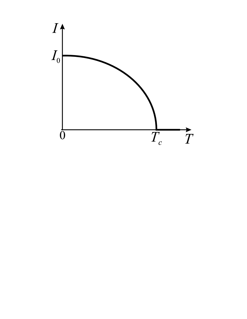
Figure 2: Typical temperature dependence of the spontaneous magnetization $I$($T$) defined as a solution of the equation (50).

Now we describe in the framework of our approach (i.e. remaining in the basis of states {$|NC\rangle$}) a model of the ferromagnetism of electron gas. For this purpose, we introduce the additional Hamiltonian of the spin-spin interaction $\widehat{H}_{ss}$. The presence of this additional Hamiltonian leads (at certain conditions) to the spontaneous magnetization, when the states with non-zero macroscopic magnetic moment become energetically preferable.

Then, for the sake of simplicity we will use the standard method of molecular (or mean) field, assuming the existence of the internal magnetic field ${\bf B}_{mol}$=$\lambda$${\bf I}$, which is proportional to the magnetization ${\bf I}$=${\bf M}$$/V$, and $\lambda$ is the Weiss coefficient. In the framework of this approach the Hamiltonian $\widehat{H}_{ss}$ can be written as:

$$\widehat{H}_{ss}=-2\mu_{B}\lambda({\bf I}\cdot\widehat{\bf S}^{(s)})\,,$$ (48)

where $\widehat{\bf S}^{(s)}$ is the spin operator of the ensemble of fermions. Choosing the quantization axis $z$ along the magnetization vector ${\bf I}$, the expresion for (48) can be rewritten in the following way:

$$\widehat{H}_{ss}=-\frac{4G_{ss}}{V\hbar^{2}}\langle\widehat{S}^{(s)}_{z}\rangle\widehat{S}^{(s)}_{z}\,,$$ (49)

where $G_{ss}$=$\hbar^{2}$$\mu^{2}_{B}$$\lambda$ is the interaction constant, and $\widehat{S}^{(s)}_{z}$ is the $z$-projection of the spin operator.

The presence of the mean field ${\bf B}_{mol}$ in combination with (44) leads to the equation

$$I=\frac{\exp\left\{\frac{2\mu_{B}{\lambda}I}{k_{B}T}\right\}-\exp\left\{-\frac{2\mu_{B}{\lambda}I}{k_{B}T}\right\}}{1+\exp\left\{\frac{2\mu_{B}{\lambda}I}{k_{B}T}\right\}+\exp\left\{-\frac{2\mu_{B}{\lambda}I}{k_{B}T}\right\}}\,I_{0}\,.$$ (50)

The spontaneous magnetization $I$=$|{\bf I}|$ as a function of the temperature $T$ is found from the solution of this equation. The typical dependence $I$($T$) is shown in Fig.2. The maximal magnetization $I_{0}$ is equal to:

$$I_{0}=\mu_{B}n\,\frac{\overline{\delta{\cal N}}}{{\cal N}}\,.$$ (51)

It should be stressed that though the result (50) coincides formally with the mean field result for the Heisenberg ferromagnetic with localized magnetic ions, but in our case we deal with the magnetic ordering of the collective conductivity electrons (if one keep in mind the description of the magnetism in metals). Note also, that the magnetic ordering of the conductivity electrons, according to our model, automatically leads to the small fractional value

$$\frac{I_{0}}{\mu_{B}n}=\frac{\overline{\delta{\cal N}}}{{\cal N}}\ll 1\,,$$ (52)

i.e. of the magnetic moment in the $\mu_{B}$ units per one electron.

As it follows from (50), at $T$=0 the spontaneous magnetization does exist (and it equals to $I_{0}$) for arbitrary value of the coefficient $\lambda>0$ (formally it can be as small as one likes), and, consequently, for arbitrary value of the interaction constant $G_{ss}$$>$0 in (49). This circumstance is connected with the specific dispersion law (A68)-(A69), which leads automatically to the fact that the energy of CPT-like states is the lowest energy (see Appendix). This fact, in its turn, allows us to construct the above model of the magnetism in the ensemble of fermions, based on the basis of states {$|NC\rangle$}.

However for the more realistic quadratic dispersion law (34) we can not use the formulas given above for arbitrary $\lambda$$>$0 ($G_{ss}$$>$0), because the energy $E_{NC}$ lies above the energy of the Fermi-sphere $E_{F}$ (see (35)-(37)), i.e. the states {$|NC\rangle$} is not the lowest energy states (for Hamiltonian $\widehat{H}_{BCS}$). Therefore to justify our approach it is necessary that the negative contribution to the energy of some CPT-like states due to the spin-spin interaction (49) compensates the positive additional term in the kinetic energy $\Delta E_{NC}$ (see (37)). In this case the energy of such CPT-like states will be lower than the energy of the Fermi-sphere $E_{F}$, which gives us the ground to use the basis {$|NC\rangle$} in the description of the magnetism for the quadratic dispersion law too.

It is obvious that the state $|NC,...\hat{\gamma}^{{\dagger}}_{-1,\bf k}...\rangle$, formed by the construction (46), where the spins of all the vector Cooper pairs are oriented in the same direction, acquires the maximal value of the negative addition to the energy due to the spin-spin interaction. This state has the largest spin moment $S_{z}$=$\hbar\overline{\delta{\cal N}}$/2 and the corresponding negative correction to the energy $H^{(m)}_{ss}$$<$0 (at zero temperature $T$=0) is equal to:

$$H^{(m)}_{ss}\equiv\langle NC,...\hat{\gamma}^{{\dagger}}_{-1,\bf k}...|\widehat{H}_{ss}|NC,...\hat{\gamma}^{{\dagger}}_{-1,\bf k}...\rangle=$$

$$-\frac{G_{ss}\overline{\delta{\cal N}}^{\,2}}{V}=-9\,G_{ss}\left(\frac{\Delta}{k_{F}}\right)^{2}n{\cal N}\,,$$ (53)

where the particle density $n$ can be expressed in terms of the radius of the Fermi-sphere as $n$=$k_{F}^{3}$/$3\pi^{2}$ (in the case of the quadratic dispersion law). In order to the absolute value of the negative correction (IV) exceeds the energy addition (37), the following condition should be satisfied:

$$G_{ss}\rho_{F}>1\,,$$ (54)

where the parameter $\rho_{F}$=$m$$k_{F}$/$\pi^{2}$$\hbar^{2}$ is the state density near the Fermi surface. In this case the inequality takes place

$$E_{NC}+H^{(m)}_{ss}<E_{F}$$ (55)

and, due to this reason, (54) can be considered as a criterion of the applicability of our model, when for the description of magnetic ordering near $T$=0 we can use the set of wavefunctions {$|NC\rangle$}.

It should be noted that (54) formally coincides with the criterion of ferromagnetism in the Stoner model Stoner . This circumstance is connected with the use of the state $|NC,...\hat{\gamma}^{{\dagger}}_{-1,\bf k}...\rangle$ in the deduction of (54). From the other hand, namely this state describe the case, when the spins of all fermions in the spherical layer $k_{F}$$-$$\Delta$$\leq$$k$$\leq$$k_{F}$$+$$\Delta$ are oriented along the same direction, that, in its turn, corresponds to two different (i.e. with different radiuses) Fermi-spheres. Indeed, for particles with the spin up ($\uparrow$) the corresponding radius of Fermi-sphere is $k_{F\uparrow}$=$k_{F}$$-$$\Delta$, and for particles with the spin down ($\downarrow$) we have $k_{F\downarrow}$=$k_{F}$$+$$\Delta$ (i.e. $k_{F\downarrow}$$\neq$$k_{F\uparrow}$). But namely similar approach is used in the description of the ferromagnetism in the Stoner model.

Despite the formal identity of the criterion (54) to the Stoner criterion of ferromagnetism Stoner , our approach has several principal distinctions. For example, in our approach the magnetism is governed first of all by the redistribution of fermions within the thin layer ${\bf k}$$\in$${\cal D}_{F}$ near the Fermi-sphere. This leads automatically to the small value of the magnetic moment (52) per one particle (for instance, per one conductivity electron in metal). This result as whole does not contradict to the experimental data, according to which for the overwhelming majority of metallic magnetics the magnetic moment, originating from the conductivity electrons, does not exceed few percent of the value $\mu_{B}$ per one free electron. Note also that the presence of the thin layer ${\cal D}_{F}$ in the ensemble of fermions is caused, according to our approach (i.e. in the framework of the general BCS ideology), by the interaction (scattering) with some other particles (for example, photons, phonons, excitons etc.). Apart from this, the existence of such thin layer can be connected with the presence of the energy gap near the Fermi-surface.

However the main distinguishing feature of our approach is connected with the description of the magnetic properties of conductivity electrons in the framework of notion of a gas of particles with the spin 1. In this case we can use the CPT-like states with the non-zero total momentum $|NC({\bf K})\rangle$ also, i.e. when the Fermi-sphere is constructed around the non-zero wavevector ${\bf K}$ (the momentum and energy of these states are defined by (41) and (42)). Since the states $|NC({\bf K})\rangle$ carry the magnetic moment, then these states can be interpreted as spin waves for the conductivity electrons. Moreover, since the CPT-like states are constructed according to the type of free vector particles, then a notion of a gas of Bose-particles, which are Cooper pairs with spin 1 and electric charge $2e$, emerges naturally in the description of magnetic properties. This conception can be realized by the introduction of the operators of creation of particles $\hat{\gamma}^{{\dagger}}_{q}({\bf K})$ with the spin projection $\hbar$$q$ ($q$=0,$\pm 1$) and wavevector ${\bf K}$. Due to the quadratic in ${\bf K}$ dispersion law in (42), the dispersion law for the vector particles is naturally presented as quadratic:

$$\tilde{\varepsilon}({\bf K})=\frac{(\hbar{\bf K})^{2}}{2\widetilde{m}}\,,$$ (56)

where $\widetilde{m}$ is the effective mass of the pair. These Bose-particles can form a base of conception of the magnons (i.e. on the elementary excitations of spin waves) with the spin $S$=1 in the subsystem of conductivity electrons. Also there is, in principle, the possibility of the Bose-Einstein condensation.

Our model can be extended to the case, allowing an ordering of the electron angular moments (spins) of the moveless ions in solids and their spin interaction with the conductivity electrons. We will describe this interaction by the Hamiltonian $\widehat{H}_{fs}$:

$$\widehat{H}_{fs}=\frac{A_{fs}}{V\hbar^{2}}\,(\widehat{\bf S}^{(f)}\cdot\widehat{\bf S}^{(s)})\,,$$ (57)

where $\widehat{\bf S}^{(f)}$ is the spin operator of the localized electrons (i.e. of the moveless ions), and $A_{fs}$ is the interaction constant. The total spin of one ion is denoted as $J_{f}$, and the spatial density of ions is equal to $n_{f}$.

In the model of mean field the Hamiltonian (57) can be rewritten in the form

$$\widehat{H}_{fs}=\frac{A_{fs}}{V\hbar^{2}}\,(\langle\widehat{S}^{(f)}_{z}\rangle\cdot\widehat{S}^{(s)}_{z})\,,$$ (58)

where the axis $z$ is directed along the vector of mean spin of ions ${\bf S}^{(f)}$=$\langle\widehat{\bf S}^{(f)}\rangle$.

The maximal negative energy term $H^{(m)}_{fs}$$<$0 due to the Hamiltonian (58) for the set of CPT-states {$|NC\rangle$} is achieved in the case when the spins of all ions are oriented in the same directions ($\langle\widehat{S}^{(f)}_{z}\rangle$=$\hbar$$J_{f}$$n_{f}V$), and the spins of all vector pairs are oriented parallel (at $A_{fs}$$<$0) to the spin of ions, or antiparallel (at $A_{fs}$$>$0) to the spin of ions. Take for the specificity $A_{fs}$$>$0. In this case

$$H^{(m)}_{fs}= \langle NC,...\hat{\gamma}^{{\dagger}}_{-1,\bf k}...|\widehat{H}_{fs}|NC,...\hat{\gamma}^{{\dagger}}_{-1,\bf k}...\rangle=$$ (59)

$$-A_{fs}J_{f}n_{f}\overline{\delta{\cal N}}/2\,.$$

Now the more general (with respect to (55)) condition of applicability of our model at $T$=0 can be written as

$$E_{NC}+H^{(m)}_{ss}+H^{(m)}_{fs}<E_{F}\,,$$ (60)

which leads to

$$\left(\frac{J_{f}}{6}\frac{n_{f}}{n}\frac{k_{F}}{\Delta}\,|A_{fs}|+G_{ss}\right)\rho_{F}>1\,.$$ (61)

This inequality due to the condition $k_{F}/\Delta\gg 1$ can be satisfied for sufficiently small values $A_{fs}$ even at $G_{ss}$=0.

As a whole, the described above approach to the magnetism in the ensemble of fermions corresponds to the following formal scheme. Let us consider the Hamiltonian of general form:

$$\widehat{H}=\widehat{H}_{BCS}+\widehat{\cal H}_{(S)}\,,$$ (62)

where the Hamiltonian $\widehat{\cal H}_{(S)}$ contains the interactions with the spin of particles, i.e. the interactions connected with the magnetism. For example:

$$\widehat{\cal H}_{(S)}=\widehat{H}_{ss}+\widehat{H}_{fs}+2\mu_{B}({\bf B}\cdot\widehat{\bf S}^{(s)})\,.$$ (63)

The Hamiltonian $\widehat{H}_{BCS}$ in (62) plays a role of the basic Hamiltonian, and the operator $\widehat{\cal H}_{(S)}$ is considered as a perturbation. Then, in the linear approximation we find the maximal negative correction $H_{(S)}^{(m)}$$<$0 to the energy of CPT-like states:

$$H_{(S)}^{(m)}=\langle NC,...\hat{\gamma}^{{\dagger}}_{-1,\bf k}...|\widehat{\cal H}_{(S)}|NC,...\hat{\gamma}^{{\dagger}}_{-1,\bf k}...\rangle\,.$$ (64)

From consideration of the minimality of energy we find the criterion of applicability of our model at $T$=0:

$$E_{NC}+H_{(S)}^{(m)}<E_{F}\,.$$ (65)

The inequalities (55) and (60) (correspondingly, (54) and (61)) should be considered as some particular cases of the general inequality (65). Note, the spin Hamiltonian $\widehat{\cal H}_{(S)}$ in (62) does not influence (in the linear approximation) on the energy $E_{F}$ of the Fermi state $|F\rangle$ (see (32)), because this state correspond to the zero total spin (and orbital angular momentum).

It should be noted, that in the framework of described approach one can consider (at least formally) also the case of interparticle attraction, i.e. $g$$<$0 in (8). However in this case the ground state energy of the BCS theory $E_{BCS}$ (see Bar ) lies below the Fermi energy, i.e. $E_{BCS}$$<$$E_{F}$. Due to this reason at $g$$<$0 the criterion of applicability of our model of the magnetism, based on the CPT-like states, differs from (65) and has the following form:

$$E_{NC}+H_{(S)}^{(m)}<E_{BCS}\,.$$ (66)

V CPT-like state and superfluidity in ³He

Apart from the delocalized electrons in metals another object, to which the obtained results can be related, is liquid ³He. Atoms of ³He are fermions with the spin 1/2 and due to this reason the use of the standard BSC Hamiltonian (8) for theoretical description is well-grounded (at lest, on the qualitative level).

As is known (see, for example, the reviews Mineev ; Volovik and references therein), the superfluid phase of ³He is characterized by the formation of Cooper pairs with the spin $S$=1. This fact, according to our approach, can be interpreted as a consequence of the repulsion ($g$$>$0) caused by the $s$-wave scattering, when the vector pairing can be energetically favorable. Note that the $s$-wave scattering is included in the Hamiltonian (8).

This fact, according to our approach, can be interpreted, for example, as a consequence of the effective repulsion between quasiparticles in liquid ³He, i.e. when $g$$>$0 and the vector pairing can be energetically favorable.

Note, that the operator constructions of general form (38) allow the formation of spherically asymmetrical states $|NC\rangle$, i.e. the states with the non-zero orbital angular momentum. Therefore there exists a possibility to describe paired states, which are characterized not only by the spin $S$=1, but also by the orbital momentum $L$$\neq$0 and, in particular, $L$$=$1. Here we deal with the angular orbital momentum of the relative motion of particles in the pair. The orbital momentum connected with the translational motion of the Cooper pairs is described by the states $|NC({\bf K})\rangle$ with the non-zero total linear momentum (see (41) and(42)) and by their coherent superpositions.

Thus, our approach can be considerably easily inserted into the existed general picture of the theoretical description of ³He based on the notion of Cooper pairs with $S$=1 and $L$$=$1. Basing on this notion, we can now introduce additional interaction Hamiltonians (between vector pairs, spin-orbit coupling, spin-spin, with magnetic field etc.), and allow for the more detail description of physical properties (for instance, the classification of superfluid phases in ³He-$B$, ³He-$A$, and ³He-$A_{1}$). In other words, the obtained CPT-like states can be considered, in a formally consistent way, as the zero approximation (corresponding to the spin $S$=1 of Cooper pairs) to the standard theoretical scheme.

Let us add that since the BCS model is used in the description of neutron stars (see in the review Ginz ), then the substance of neutron stars can be, in principle, an object of application of the obtained results (including the magnetism).

VI Conclusion

In the framework of standard mathematical BCS model we have considered the ensemble of interacting fermions with the spin 1/2. Usually this model is used for the description of Cooper pairs with the total spin $S$=$\,0$. However, as it turns out, the standard BCS Hamiltonian describes also the vector ($S$=1) pairing of particles with the opposite linear momenta close to the Fermi sphere. Thus, it is shown that, in principle, for the description of vector Cooper pairs with the spin 1 it is not necessary to introduce into the interaction Hamiltonian the corresponding vector operator constructions, i.e. it is possible to remain in the framework of the operator (8), formed only by the scalar constructions (II). The found states nullify the interaction Hamiltonian (8) and, therefore, they have some analogy with the known CPT effect. Moreover, there are good reasons to believe that at certain conditions these CPT-like states can belong to the lower part of energy spectrum, and, consequently, play a significant role in the description of physical properties of the given ensemble.

Since the CPT-like states have a huge degree of degeneracy and carry the macroscopic magnetic moment, then it is logical to apply them to the description of the magnetic ordering for the delocalized electrons in the case $g$$>$0, when the vector pairing is energetically favorable. In particular, we have proposed a new approach to the explanation of the ferromagnetism (and the magnetic ordering in general) connected with the delocalized electrons (i.e. itinerant magnetism). Moreover, here the concept of magnons with the spin $S$=1 in the subsystem of the delocalized electrons naturally emerges. Apart from the magnetism in metals (conductors), the obtained results may have a potential significance for the description of the superfluidity in ³He, explaining, for example, the vector type ($S$=1) of Cooper pairs as a consequence of the repulsion ($g$$>$0) in the interaction Hamiltonian (8).

Thus, there are serious reasons to assume that the standard mathematical BCS model is more universal and, apart from the superconductivity (at $g$$<$0) it can serve as a base in the description of other affects in metals (conductors) and in quantum Fermi liquids (for example, at $g$$>$0).

The presented results on the magnetism in metals and the superfluidity in ³He are preliminary (discussional) and have a character of a review of some possible consequences under the assumption that the found CPT-like states have a concrete physical sense and they can belong to the lower part of energy spectrum. However, even such a qualitative analysis confirms that the proposed approach deserves an attention and further development.

Authors thank G.I. Surdutovich, E.G. Batyev, L.V. Il’ichev, and A.M. Tumaikin for useful discussions. This work was supported by grants INTAS-SBRAS (06-1000013-9427), RFBR (07-02-01230, 07-02-01028, 08-02-01108), and Presidium SB RAS.

Appendix A

Let us show that at some simplifying assumptions on the operators (6) and (8) the energy level $E_{NC}$ is the ground level at $g$$>$0.

So in the interaction Hamiltonian (8) we will assume the equality $G$$({\bf k}_{1},$${\bf k}_{2})$=1 for the formfactor. Then the operator $\widehat{W}$ can be written in the form:

$$\widehat{W}=g\,\widehat{B}^{{\dagger}}\widehat{B}\,,$$ (A67)

$$\widehat{B}=\frac{1}{\sqrt{V}}\sum_{{\bf k}\in{\cal D}_{F}}\hat{a}_{\downarrow-{\bf k}}\hat{a}_{\uparrow{\bf k}}\,.$$

Another approximation is related to the dispersion law $\varepsilon_{\bf k}$ in the unperturbed Hamiltonian (6). for the thin spherical layer ${\cal D}_{F}$ (when $\Delta$$\ll$$k_{F}$) the energy of particles $\varepsilon_{\bf k}$ with different ${\bf k}$ are almost the same and, due to this reason, we will assume their equality $\varepsilon_{\bf k}$=$\bar{\varepsilon}$ for all ${\bf k}$$\in$${\cal D}_{F}$. In this case the kinetic energy operator $\widehat{H}_{0}$ is split into the two summand:

$$\widehat{H}_{0}=\bar{\varepsilon}\,\widehat{\delta{\cal N}}+\widehat{H}^{(\Phi)}_{0}\,,\\$$ (A68)

Here the first summand corresponds to the states with $(k_{F}$$-$$\Delta)$$<$$|{\bf k}|$$<$$(k_{F}$$+$$\Delta)$ and it is proportional to the operator of the particle number in the spherical layer ${\cal D}_{F}$:

$$\widehat{\delta{\cal N}}=\sum_{s,{\bf k}\in{\cal D}_{F}}\hat{a}^{{\dagger}}_{s{\bf k}}\hat{a}_{s{\bf k}}\,.$$ (A69)

The dispersion law $\varepsilon_{\bf k}$ for $|{\bf k}|$$<$$(k_{F}$$-$$\Delta)$ in the second summand $\widehat{H}^{(\Phi)}_{0}$ in (A68) is assumed arbitrary:

$$\widehat{H}^{(\Phi)}_{0}=\sum_{s,|{\bf k}|<(k_{F}-\Delta)}\varepsilon_{\bf k}\,\hat{a}^{{\dagger}}_{s{\bf k}}\hat{a}_{s{\bf k}}\,.$$ (A70)

Take arbitrary eigenvector $|\Psi\rangle$ for the total Hamiltonian $\widehat{H}_{BCS}$=$\widehat{H}_{0}$$+$$\widehat{W}$, i.e. $\widehat{H}_{BCS}$$|\Psi\rangle$=$E$$|\Psi\rangle$. Then, in view of (A68) and (A67), for the eigenenergy $E$ the following relationships is fulfilled:

$$E=\langle\Psi|\widehat{H}_{BCS}|\Psi\rangle=\langle\Psi|\widehat{H}_{0}|\Psi\rangle+g\,\langle\Psi|\widehat{B}^{{\dagger}}\widehat{B}|\Psi\rangle=$$

$$\bar{\varepsilon}\,\langle\Psi|\widehat{\delta{\cal N}}|\Psi\rangle+\langle\Psi|\widehat{H}^{(\Phi)}_{0}|\Psi\rangle+g\,\langle\Psi|\widehat{B}^{{\dagger}}\widehat{B}|\Psi\rangle\,.$$ (A71)

By the problem statement we are interested only in such states, which can be symbolically presented as:

$$|\Psi\rangle=\widehat{\Psi}\,\widehat{\Phi}(\Delta)\,|0\rangle\,,\quad\langle\Psi|\Psi\rangle=1\,,$$ (A72)

where some operator $\widehat{\Psi}$ acts only on the states in the spherical layer ${\bf k}$$\in$${\cal D}_{F}$, and the fixed construction $\widehat{\Phi}$($\Delta$) in accordance with (23) describes the fully occupied states with $|{\bf k}|$$<$$(k_{F}$$-$$\Delta)$. Since the kinetic energy operator (A70) also acts only on the states with $|{\bf k}|$$<$$(k_{F}$$-$$\Delta)$, then for arbitrary vector $|\Psi\rangle$ the second summand in (A) is fixed:

$$\langle\Psi|\widehat{H}^{(\Phi)}_{0}|\Psi\rangle=E_{\Phi}\,.$$ (A73)

Apart from this, only the states with conserved number of particles (at least in average) are physically significant, i.e. the average of the particle number operator $\widehat{N}$=$\sum_{s,{\bf k}}\hat{a}^{{\dagger}}_{s{\bf k}}\hat{a}_{s{\bf k}}$ is equal to the fixed number ${\cal N}$:

$$\langle\Psi|\widehat{N}|\Psi\rangle={\cal N}\,.$$ (A74)

From the other hand, the construction $\widehat{\Phi}$($\Delta$) determines the fixed number ${\cal N}_{\Phi}$ of particles, occupying the sphere with $|{\bf k}|$$<$$(k_{F}$$-$$\Delta)$. Consequently, all the physically significant states $|\Psi\rangle$ should also conserve the particle number $\overline{\delta{\cal N}}$ in the spherical layer ${\cal D}_{F}$, because ${\cal N}$=${\cal N}_{\Phi}$$+$$\overline{\delta{\cal N}}$. As a result we have:

$$\langle\Psi|\widehat{\delta{\cal N}}|\Psi\rangle=\overline{\delta{\cal N}}\,.$$ (A75)

Using (A73) and (A75), the expression (A) can be rewritten in the following form:

$$E=\bar{\varepsilon}\,\overline{\delta{\cal N}}+E_{\Phi}+g\,\langle\Psi|\widehat{B}^{{\dagger}}\widehat{B}|\Psi\rangle\,.$$ (A76)

Consider now the case $g$$>$0. From the obvious inequality

$$\langle\Psi|\widehat{B}^{{\dagger}}\widehat{B}|\Psi\rangle=\langle\widehat{B}\Psi|\widehat{B}\Psi\rangle\geq 0\,,$$ (A77)

it follows that

$$E\geq\bar{\varepsilon}\,\overline{\delta{\cal N}}+E_{\Phi}\,.$$ (A78)

From the other hand, since the CPT-like states nullify the interaction operator $\widehat{W}$, then for the energy $E_{NC}$ we get:

$$E_{NC}=\bar{\varepsilon}\,\overline{\delta{\cal N}}+E_{\Phi}\,.$$ (A79)

Thus, the states $|NC\rangle$ belong to the ground energy level, as we wished prove.

Moreover, let us show that the energy of all other states lie above the energy $E_{NC}$. Indeed, consider the eigenstate $|\Psi\rangle$, for which the condition of nullification of the operator $\widehat{W}$ is not fulfilled, i.e. $\widehat{W}$$|\Psi\rangle$$\neq$0. In accordance with (A67) this means $\widehat{B}$$|\Psi\rangle$$\neq$0. Then the rigorous inequality is fulfilled

$$\langle\Psi|\widehat{B}^{{\dagger}}\widehat{B}|\Psi\rangle=\langle\widehat{B}\Psi|\widehat{B}\Psi\rangle>0\,,$$ (A80)

which, in its turn, leads to the rigorous inequality $E$$>$$E_{NC}$.

Vice versa, in the case $g$$<$0 it can be proved analogously that the energy $E_{NC}$ is maximal.

It should be noted that although the model dispersion law for free particles in (A68) is approximate, nevertheless, the performed analysis argues that our statement that the vector pairing ($S$=1) is possibly energetically favorable for $g$$>$0 is not unfounded. Vice versa, in the case of interparticle attraction ($g$$<$0) the vector type of pairing is not energetically favorable.

Let us add that above we talk only about the states $|NC\rangle$, because we know their exact analytical form and energy $E_{NC}$. It is well to bear in mind that in the general case there exist a whole family of allied energy levels, which will be denoted as $\{NC\}$. For example, if in the operator construction $\widehat{\Psi}_{NC}$ (see (29)) we replace several operators $\hat{\gamma}^{{\dagger}}_{q_{\bf k},{\bf k}}$ by some other constructions, consisting of $\hat{a}^{{\dagger}}_{s,{\bf k}}$ (conserving the total particle number ${\cal N}$), then as a result we will generate some state $|\Psi\rangle$, which formally does not obey the condition (11), i.e. $\widehat{W}$$|\Psi\rangle$$\neq$0. At the same time, it is obvious that the state $|\Psi\rangle$ does not practically differ from the state $|NC\rangle$ (especially in the limit ${\cal N}$$\to$$\infty$). The definition of the family (sub-band) of levels $\{NC\}$ is a subject of special consideration. Generally speaking the states from $\{NC\}$ should be characterized by the predominance of Cooper pairs with the spin $S$=1, and by the considerably weak influence of the operator $\widehat{W}$ on them. It should be noted, that the similar situation appears in the standard CPT effect in the resonant interaction of light with multilevel atoms. In this case there are one or several exact CPT-states and a whole family of allied states (with similar physical properties and close energy). Thus, the exact CPT-states play a role of a kernel-type of special subsystem of levels.

References

- (1) G. Alzetta, A. Gozzini, L. Moi, and G. Orriols, Nuovo Cimento Soc. Ital. Fis. B 36, 5 (1976).
- (2) E. Arimondo and G. Orriols, Lett. Nuovo Cimento Soc. Ital. Fis. 17, 33 (1976).
- (3) H. R. Gray, R. M. Whitley, and C. R. Stroud, Opt. Lett. 3, 218 (1978).
- (4) B. D. Agap’ev, M. B. Gornyi, B. G. Matisov, Yu. V. Rozhdestvensky, Uspekhi Fiz. Nauk 163, 35 (1993).
- (5) E. Arimondo, in Progress in Optics, E. Wolf ed. XXXV, 257 (1996).
- (6) P. R. Hemmer, S. Ezekiel, and C. C. Leiby, Jr. Opt. Lett. 8, 440 (1983).
- (7) A. Akulshin, A. Celikov, and V. Velichansky, Opt. Commun. 84, 139 (1991).
- (8) M. O. Scully and M. Fleischhauer, Phys. Rev. Lett. 69, 1360 (1992).
- (9) J. Kitching, S. Knappe, L. Vukicevic, L. Hollberg, R. Wynands, and W. Weidman, IEEE Trans. Instrum. Meas. 49, 1313 (2000).
- (10) S. E. Harris, Physics Today, 50(7), 36 (1997).
- (11) O. Kocharovskaya, Phys. Rep. 129, 175 (1992).
- (12) M. O. Scully, Phys. Rep. 129, 191 (1992).
- (13) A. Aspect, E. Arimondo, R. Kaiser, N. Vansteenkiste, and C. Cohen-Tannoudji, Phys. Rev. Lett. 61, 826 (1988).
- (14) A. Aspect, E. Arimondo, R. Kaiser, N. Vansteenkiste, and C. Cohen-Tannoudji, J. Opt. Soc. Amer. B 6, 2112 (1989).
- (15) P. Marte, P. Zoller, and J. L. Hall, Phys. Rev. A 44, 4118 (1991).
- (16) M. Weitz, B. C. Young, and S. Chu, Phys. Rev. Lett. 73, 2563 (1994).
- (17) P. D. Featonby, G. S. Summy, C. L. Webb, R. M. Godun, M. K. Oberthaler, A. C. Wilson, C. J. Foot, and K. Burnett, Phys. Rev. Lett. 81, 495 (1998).
- (18) I. E. Masets and B. G. Matisov, Pis’ma v Zh. Eksp. Teor. Fiz. 64, 483 (1996).
- (19) M. Fleschauer and M. D. Lukin, Phys. Rev. Lett. 84, 5094 (2000).
- (20) M. Fleschauer and M. D. Lukin, Phys. Rev. A 65, 022314 (2002).
- (21) C. Liu, Z. Dutton, C. H. Behroozi, and L. V. Hau, Nature 409, 490 (2001).
- (22) D. F. Phillips, A. Fleischhauer, A. Mair, R. L. Walsworth, and M. D. Lukin, Phys. Rev. Lett. 86, 783 (2001).
- (23) A. S. Zibrov, A. B. Matsko, O. Kocharovskaya, Y. V. Rostovtsev, G. R. Welch, and M. O. Scully, Phys. Rev. Lett. 88, 103601 (2002).
- (24) C. H. van der Wal, M. D. Eisaman, A. Andre, R. L. Walsworth, D. F. Phillips, A. S. Zibrov, and M. D. Lukin, Science 301, 196 (2003).
- (25) F. T. Hioe and C. E. Carroll, Phys. Rev. A 37, 3000 (1988).
- (26) V. S. Smirnov, A. M. Tumaikin, and V. I. Yudin, Zh. Eksp. Teor. Fiz. 96, 1613 (1989).
- (27) A. M. Tumaikin and V. I. Yudin, Zh. Eksp. Teor. Fiz. 98, 81 (1990).
- (28) A. V. Taichenachev, A. M. Tumaikin, and V. I. Yudin, Europhys. Lett. 45, 301 (1999).
- (29) A. V. Taichenachev, A. M. Tumaikin, and V. I. Yudin, Zh. Eksp. Teor. Fiz. 118, 77 (2000).
- (30) A. V. Taichenachev, A. M. Tumaikin, and V. I. Yudin, Pis’ma v Zh. Eksp. Teor. Fiz. 79, 75 (2004).
- (31) A. V. Taichenachev, A. M. Tumaikin, and V. I. Yudin, Europhys. Lett. 72, 562 (2005).
- (32) Ch. Bolkart, R. Weiss, D. Rostohar, and M. Weitz, Laser Phys. 15, 3 (2005).
- (33) A. M. Tumaikin and V. I. Yudin, Physica B 175, 161 (1991).
- (34) J. Bardeen, L. N. Cooper, and J. R. Schriffer, Phys. Rev. 108, 1175 (1957).
- (35) A. V. Taichenachev and V. I. Yudin, arXiv:quant-ph/0610012 (2006).
- (36) P. W. Anderson and P. Morel, Phys. Rev. Lett. 5, 136 (1960).
- (37) L. P. Gor’kov and V. M. Galitsky, Zh. Eksp. Teor. Fiz. 40, 1124 (1961).
- (38) V. G. Vaks, V. M. Galitsky, and A. I. Larkin, Zh. Eksp. Teor. Fiz. 42, 1319 (1962).
- (39) I. A. Privorotsky, Zh. Eksp. Teor. Fiz. 43, 2255 (1962).
- (40) A. I. Larkin, Pis’ma v Zh. Eksp. Teor. Fiz. 5, 205 (1965).
- (41) E. G. Stoner, Proc. Roy. Soc. A165, 372 (1938).
- (42) V. P. Mineev, Uspekhi Fiz. Nauk 139, 303 (1983).
- (43) G. E. Volovik, Uspekhi Fiz. Nauk 143, 73 (1984).
- (44) V. L. Ginzburg, Uspekhi Fiz. Nauk 97, 601 (1969).