Subspace Confinement: How Good is your Qubit?

Abstract

The basic operating element of standard quantum computation is the qubit, an isolated two-level system that can be accurately controlled, initialized and measured. However, the majority of proposed physical architectures for quantum computation are built from systems that contain much more complicated Hilbert space structures. Hence, defining a qubit requires the identification of an appropriate controllable two-dimensional sub-system. This prompts the obvious question of how well a qubit, thus defined, is confined to this subspace, and whether we can experimentally quantify the potential leakage into to states outside the qubit subspace. In this paper we demonstrate that subspace leakage can be quantitatively characterized using minimal theoretical assumptions by examining the Fourier spectrum of the oscillation experiment.

I Introduction

The issue of subspace confinement for qubit systems is fundamental to the primary operating assumptions of quantum processors. The concepts of universality, quantum gate operations, algorithms, error correction and fault-tolerant computation hinge on the precept that the fundamental quantum system is an isolated, controllable, two-dimensional system (qubit).

It is well known that most of the physical realizations of qubits are in fact multi-level quantum systems, which can theoretically be confined to a two-dimensional (qubit) subspace. Important examples range from super-conducting qubits SC1 ; SC2 ; SC3 to atomic systems such as cavity-coupled color centers NV1 ; NV2 ; NV3 and ion traps ion1 . In the former systems, a qubit is generally defined as the subspace (of the full Hilbert space) spanned by the two lowest energy states in an arbitrarily shaped potential such as the washboard potential of current-biased Josephson Junctions wash1 ; wash2 . However, the potential number of valid quantum states within each well is not limited to two, and quantum gates, especially if sub-optimally implemented, may inadvertently populate other confined states. Similarly in ion trap systems, a qubit is usually defined by two electronic states of an ion, either two hyperfine levels or a ground state and a meta-stable excited state, but once again there exist many other electronic states. Hence a more stringent definition of a qubit would consist of a two-level quantum system with classical control confined to the unitary group $SU(2)$.

The ability to initialize, operate and measure completely within the two-level subspace representing “the qubit” is vital to the successful operation of any large scale device constructed from such quantum systems. Standard quantum error correction protocols (QEC) QEC1 ; QEC2 ; QEC3 generally assume that the qubit system is precisely confined to the two-level subspace and that all quantum gates operate only on the qubit degrees of freedom. If poor control or environmental influences inadvertently results in non-zero population of higher levels, leakage correction protocols are necessary.

The issue of subspace leakage in quantum processing has been addressed in depth from the standpoint of error correction. Work by Lidar Lidar1 ; Lidar2 examined the construction of Leakage Reduction Units (LRU’s), which use modified pulsing techniques to ensure that any unitary dynamics outside the qubit subspace can be compensated for which has been adapted specifically for super-conducting systems mass . Another type of LRU’s uses quantum teleportation tele1 to map a multi-level quantum state back to a freshly initialized two-level qubit. Finally, active detection such as non-demolition measurements (which detect population in non-qubit states without discriminating between the qubit states) can be performed on the system det1 ; det2 ; det3 ; det4 . If an out-of-subspace detection event occurs the leaked qubit is re-initialized or replaced. The inclusion of LRU’s based on teleportation has been investigated within the context of fault-tolerant quantum computation alifredis and shows that, in principle, the inclusion of leakage protection does not adversely affect large scale concatenated error correction.

Although these schemes are viable methods to detect and correct for improperly confined qubit dynamics, they can be cumbersome to implement and many systems admit, in principle, sufficiently confined Hamiltonian dynamics so that leakage could be expected to be heavily suppressed. For example, for ion-trap qubits controlled by lasers, leakage to other ionic states can be made negligible by employing very finely tuned lasers and sufficiently long (and possibly optimally tailored) control pulses. Advances in qubit engineering may therefore allow us to eliminate or at least substantially reduce the need for laborious leakage detection/prevention schemes in many cases, provided that we can experimentally ascertain sufficiently high confinement of manufactured qubits under classically controlled Hamiltonian dynamics.

In this paper we present a simple generic protocol to estimate qubit confinement, or more precisely, establish bounds on the subspace leakage rates, for “quality control” purposes. The main goal is to allow us to empirically detect inferior qubits by using readily obtainable experimental data to derive tight bounds on the subspace leakage of the system. This protocol would represent one of the first steps towards full system characterization char1 ; char2 ; char3 ; char4 .

Section II briefly outlines the basic assumptions with respect to the measurement and control model and the motivation for the proposed protocol. Section III discusses the basic mathematical properties of qubit oscillation data and shows how a minimal amount of information obtained from the oscillation spectrum can be used to derive empirical bounds on the subspace leakage rate, and that these bounds are very tight for the high quality qubits required for practical quantum computation. In section IV, the effects of finite sampling are considered and studied using numerical simulations. Section V compares the efficiency of bounding confinement using the proposed scheme versus alternative approaches such as detection of imperfect confinement by identifying additional transition peaks within the Rabi spectrum. Finally, section VI briefly examines the effects of decoherence.

II Motivation and Preliminaries

Estimation of qubit confinement represents one of the first major steps in full qubit characterization. Therefore, the protocol should not be predicated on the availability of sophisticated measurements or control, and should be amenable to automation so that it could be used in conjunction with a potentially automated qubit manufacturing process. The bounds on the subspace leakage will be based on the observable qubit evolution under an externally controlled driving Hamiltonian. We assume that our classical control switches on the single qubit dynamics and that the governing Hamiltonian is piecewise constant in time. Hence the Hamiltonian induces the unitary operator $U=e^{-iHt}$, with $\hbar=1$.

Although this assumption may not be applicable to all systems, e.g., systems subject to ultra-fast tailored control pulses, it is not as restrictive as it might appear. It is generally be valid for systems such as quantum dots or Josephson junctions subject to external potentials created by voltage gates if the gate voltages are (approximately) piecewise constant. It is also a good approximation for systems subject to time-dependent fields such as laser pulses in a regime where the rotating wave approximation (RWA) is valid and the pulse envelopes can be approximated by square-waves. In this case, the Hamiltonian relevant for our purposes is the (piecewise constant) RWA Hamiltonian determined by the amplitudes, detunings and possibly phases of the control pulses. This model can even be valid for other pulse shapes if the Hamiltonian is taken to be an average Hamiltonian describing the effective dynamics on a certain time scale (beyond which we do not resolve the time-dependent dynamics). However, the main focus of the paper is not when the dynamics of a system can be modeled in this way, but rather how to assess subspace confinement for systems where this model of the dynamics is valid.

Assuming the effective control-dependent Hamiltonian $H=H[\vec{f}]$ is constant for $0\leq t\leq t_{k}$, where $\vec{f}$ is the classical “control knob” parameter, the evolution during this time period is given by the unitary operator $U(t)=e^{-iHt}$. Although $H$ will generally depend on control inputs, we shall omit this dependence in the following for notational convenience. The driven system generally undergoes coherent oscillations, which are often referred to as Rabi oscillations, especially for optically driven systems in the RWA regime. Although our model is not limited to these systems, we shall use the terms coherent oscillations and Rabi oscillations interchangeably throughout this paper.

The measurement model assumed is crucial to the relevance of the protocol. Some standard measurement models in quantum computation assume the ability to detect both the $|0\rangle$ and $|1\rangle$ states independently (such as SET detectors in solid state designs SS1 ; SS2 ; SS3 ). In this case, estimating subspace leakage is fairly straightforward and requires only repeated measurement of the system while undergoing evolution. The leakage is simply given by the deviation of the cumulative probability of measuring $|1\rangle$ or $|0\rangle$ from unity. However, this measurement model is not realistic for the majority of proposed systems.

Color centers and ionic qubits use externally pumped transitions to discriminate between a light state ($\equiv|0\rangle$) and other “dark” states, while readout in super-conducting systems SCmeas1 ; SCmeas2 involves lowering a potential barrier such that only one of the qubit states can leak to an external detection circuit. The measurement outcome of the indirectly probed state is inferred from the non-detection of the directly measured state and for such measurement models estimating confinement is more complicated. Hence this paper utilizes the latter model in order to quantify confinement. It should be noted that we are not considering the concept of weak measurement, in each case we assume that the measurement of the system causes a full POVM collapse of the wavefunction. We also assume that the measurement apparatus has been sufficiently characterized. In order to to successfully implement computation, readout fidelity should ideally be of the same order as general systematic and decoherence errors. Therefore, characterization is initially required to ascertain the error rate associated with measurement which can then be incorporated into calculations of confinement.

Strong non-qubit transitions can still be identified directly via modulations in the Rabi oscillations data as shown in Fig. 1b for a three-state system evolving under the trial Hamiltonian

$$H_{m}=\begin{pmatrix}0&1&0.5\\ 1&1&0\\ 0.5&0&1.5\end{pmatrix}.$$ (1)

However, the Rabi oscillation data for the modified three-state Hamiltonian,

$$H_{n}=\begin{pmatrix}0&1&0.01\\ 1&1&0\\ 0.01&0&1.5\end{pmatrix},$$ (2)

depicted in Fig. 1a shows that an apparent lack of modulations in the Rabi oscillation data is not proof of perfect confinement, and that quantitative measures of confinement or subspace leakage and experimental protocols are needed.

III Estimation of subspace leakage

By defining the projection operator onto a two dimensional subspace, $\Pi=|0\rangle\langle 0|+|1\rangle\langle 1|$, subspace leakage is given by,

$$\epsilon=1-\text{Tr}[\Pi\rho],$$ (3)

with $\rho=U^{\dagger}(t)|0\rangle\langle 0|U(t)$. Unfortunately, we cannot calculate $\epsilon$ directly without knowledge of the Hamiltonian. However, we can estimate subspace leakage experimentally from standard Rabi oscillation data.

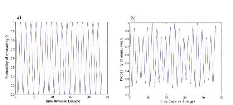
Figure 1: Modulations in the Rabi oscillations of a three-level system driven by the Hamiltonians, $H_{m}$ and $H_{n}$. Fig. b) provides clear evidence that this system is not a qubit, while Fig. a) appears to show perfect confinement. However the analysis in the following sections will show that the subspace confinement for the system in Fig. a) is also not sufficient for large-scale QIP applications.

III.1 Perfect confinement

Consider a general $N$-level system undergoing coherent evolution via a driving Hamiltonian $H_{N}$ in the closed system case of no environmental decoherence. If confinement under this Hamiltonian is perfect, $H_{N}$ has a direct sum decomposition,

$$H_{N}=H_{2\times 2}\oplus H_{(N-2)\times(N-2)}$$ (4)

where $H_{2\times 2}$ represents the control Hamiltonian confined to the qubit subspace, $\mbox{span}\{|0\rangle,|1\rangle\}$, the state $|0\rangle$ being defined by the measurement, and the excited state $|1\rangle$ by the allowed transition. For our measurement model the observed Rabi oscillations have the functional form $f(t)=|\langle 0|U_{N}(t)|0\rangle|^{2}$. As there is no coupling between the state $|0\rangle$ and states outside the $H_{2\times 2}$ subspace, we can expand $f(t)$ by diagonalizing $U_{2\times 2}(t)=\exp(-iH_{2\times 2}t)$

$$f(t) =|\langle 0|A^{\dagger}\text{diag}\{e^{-i\lambda_{0}t},e^{-i\lambda_{1}t}\}A|0\rangle|^{2}$$ (5)

$$=||c_{0}|^{2}e^{-i\lambda_{0}t}+|c_{1}|^{2}e^{-i\lambda_{2}t}|^{2}$$

$$=|c_{0}|^{4}+|c_{1}|^{4}+|c_{0}|^{2}|c_{1}|^{2}(e^{i\omega_{01}t}+e^{-i\omega_{01}t})$$

where $U_{2\times 2}(t)=A^{\dagger}e^{-iH_{d}t}A$, $A|0\rangle=c_{0}|0\rangle+c_{1}|1\rangle$, $\omega_{01}=\lambda_{0}-\lambda_{1}$ and $\{\lambda_{j}\}$ are the eigenvalues of $H_{2\times 2}$. For perfect confinement, $H_{2\times 2}$ induces coherent oscillations between the two qubit levels at a Rabi frequency given by the difference in the eigenvalues. Taking the Fourier transform of $f(t)$ gives

$$F(\omega)=\mbox{FT}[f(t)] =(|c_{0}|^{4}+|c_{1}|^{4})\delta(\omega)$$ (6)

$$+|c_{0}|^{2}|c_{1}|^{2}\delta(\omega- \omega_{01})+|c_{0}|^{2}|c_{1}|^{2}\delta(\omega+\omega_{01}).$$

Conservation of probability (total population) thus implies $(|c_{0}|^{2}+|c_{1}|^{2})^{2}=|c_{0}|^{4}+|c_{1}|^{4}+2|c_{0}|^{2}|c_{1}|^{2}=1$, and hence the heights of the two Fourier peaks for perfect confinement will satisfy the relation $h_{0}+2h_{0,1}=1$, where $h_{0}=|c_{0}|^{4}+|c_{1}|^{4}$ and $h_{0,1}=|c_{0}|^{2}|c_{1}|^{2}$.

III.2 Imperfect confinement

If the system experiences leakage to states outside the qubit subspace then the corresponding control Hamiltonian $H_{N}$ can no longer be reduced to a direct sum representation (4) but it can be diagonalized $H_{d}=\text{diag}[\{\lambda_{j}\}]$, $\{\lambda_{j}\}$ being the eigenvalues of $H_{N}$, and the propagator $U_{N}(t)$ expressed as $U_{N}(t)=A^{\dagger}e^{-iH_{d}t}A$. The Rabi data is now a linear superposition of multiple oscillations corresponding to different transitions of the $N$-level system

$$f(t) =|\langle 0|A^{\dagger}e^{-iH_{d}t}A|0\rangle|^{2}$$ (7)

$$=\bigg{|}\sum_{a=0}^{N-1}|c_{a}|^{2}e^{-i\lambda_{a}t}\bigg{|}^{2}=\sum_{a,b}|c_{a}|^{2}|c_{b}|^{2}e^{-i(\lambda_{a}-\lambda_{b})t}$$

and the corresponding peak heights in the Fourier spectrum can be expressed in terms of the expansion co-efficients, $A|0\rangle=\sum_{a=0}^{N-1}c_{a}|a\rangle$, as,

$$h_{0} =\sum_{a=0}^{N-1}|c_{a}|^{4},\quad\quad h_{a,b}=|c_{a}|^{2}|c_{b}|^{2},\quad\quad a\neq b.$$ (8)

Conservation of probability leads to

$$1=\bigg{(}\sum_{a=0}^{N-1}|c_{a} |^{2}\bigg{)}^{2}=\sum_{a=0}^{N-1}|c_{a}|^{4}+\sum_{a\neq b}|c_{a}|^{2}|c_{b}|^{2}$$ (9)

$$=h_{0}+\sum_{a\neq b}h_{a,b}.$$

Imperfect confinement implies $h_{0}+2h_{0,1}<1$. We see from this analysis that the subspace leakage $\epsilon$ is determined by the cumulative amplitudes of all non-qubit states for a given eigenstate of $H_{N}$, which can be calculated from all the peak heights in the Fourier spectrum,

$$\epsilon=\sum_{a}\sqrt{\frac{h_{a,b}h_{a,c}}{h_{b,c}}},\quad b,c\neq a.$$ (10)

However, exact calculation of $\epsilon$ requires identification of all peaks in the Fourier spectrum and knowledge of which peak corresponds to each trasition. It is therefore desirable to derive bounds on the subspace leakage that only involve a few dominant and thus easily identifiable Fourier peaks.

III.3 Bounds on subspace leakage

We can derive upper and lower bounds on $\epsilon$ using only the heights of the primary spectral peaks $h_{0}$ and $h_{0,1}$.

$$h_{0}+2h_{0,1} =(|c_{0}|^{2}+|c_{1}|^{2})^{2}+\sum_{a\neq 0,1}|c_{a}|^{4}$$ (11)

$$=\text{Tr}[\Pi\rho]^{2}+\sum_{a\neq 0,1}|c_{a}|^{4}$$

$$=(1-\epsilon)^{2}+\sum_{a\neq 0,1}|c_{a}|^{4}.$$

Provided $\sum_{a\neq 0,1}|c_{a}|^{4}\ll 1$, i.e., subspace leakage is reasonably small, we obtain a tight lower bound for $\epsilon$ as a function of only the two major peak heights:

$$h_{0}+2h_{0,1} \geq(1-\epsilon)^{2}$$ (12)

$$\therefore\quad\epsilon \geq 1-\sqrt{h_{0}+2h_{0,1}}.$$

The upper bound for $\epsilon$ can also be calculated quite easily. Recall that

$$\epsilon^{2} =\bigg{(}\sum_{a\neq 0,1}|c_{a}|^{2}\bigg{)}^{2}=\sum_{a\neq 0,1}|c_{a}|^{4}+\sum_{a,b>1,a\neq b}|c_{a}|^{2}|c_{b}|^{2}$$ (13)

$$\geq\sum_{a\neq 0,1}|c_{a}|^{4}.$$

Comparison with (11) thus immediately yields

$$h_{0}+2h_{0,1}\leq(1-\epsilon)^{2}+\epsilon^{2}=1-2\epsilon+2\epsilon^{2},$$ (14)

which can be solved for $\epsilon$

$$\epsilon\leq\frac{1}{2}(1-\sqrt{2h_{0}+4h_{0,1}-1}).$$ (15)

The other solution to Eq. (14) is invalid as a bound due to the asymptotic behavior of both the upper and lower bound

$$\lim_{(h_{0}+2h_{0,1})\rightarrow 1}\text{min}(\epsilon)=0,$$ (16)

$$\lim_{(h_{0}+2h_{0,1})\rightarrow 1}\text{max}(\epsilon)=0.$$

Since the second term in (13) represents the heights of all the Fourier peaks not associated with the $|0\rangle\leftrightarrow|1\rangle$, $|0\rangle\leftrightarrow|a\rangle$ or $|1\rangle\leftrightarrow|a\rangle$ transitions, for $|a\rangle\neq|1\rangle$. For a well confined system this is a very small correction to $\epsilon^{2}$, consequently the bound is again strong.

Therefore, the subspace leakage $\epsilon$ is bounded above and below by

$$1-\sqrt{h_{0}+2h_{0,1}}\leq\epsilon\leq\frac{1}{2}(1-\sqrt{2h_{0}+4h_{0,1}-1}).$$ (17)

Note that this double inequality involves only the two main peaks in the Fourier spectrum, i.e., we can bound the subspace leakage without determining the heights of all peaks.

For the trial Hamiltonians (1) and (2) we obtain the following bounds

$$0.0497\leq \epsilon_{H_{m}}\leq 0.0511,$$ (18)

$$3.9754\times 10^{-4}\leq \epsilon_{H_{n}}\leq 3.9762\times 10^{-4},$$

while the actual values of $\epsilon_{H_{m}}$ and $\epsilon_{H_{n}}$ are

$$\epsilon_{H_{m}}=5.11\times 10^{-2},\quad\quad\epsilon_{H_{n}}=3.9762\times 10^{-4}.$$ (19)

In both cases the upper bound for $\epsilon$ equals the actual value of $\epsilon$. This is due to the fact that both systems are of dimension three, and when estimating $\text{max}(\epsilon)$ we neglected terms of the form

$$\sum_{(a,b)\neq(0,1),a\neq b}|c_{a}|^{2}|c_{b}|^{2},$$ (20)

which naturally vanish for a three-level system.

Fig. 2 shows how the bounds (17) for $\epsilon$ converge as confinement increases ($\gamma\rightarrow 0$) for the test Hamiltonian,

$$H_{4}=\begin{pmatrix}0&1&\gamma&\gamma\\ 1&1&0&0\\ \gamma&0&1.5&0\\ \gamma&0&0&1.7\end{pmatrix}.$$ (21)

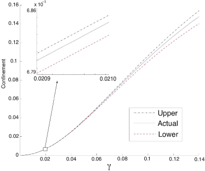
Figure 2: Upper and lower bounds on $\epsilon$ for the four-level trial system governed by the Hamiltonian (21), characterized by a static coupling between the qubit states and a variable coupling $\gamma$ to two higher levels. As $\gamma\rightarrow 0$ the subspace leakage approaches 0 and the bounds for $\epsilon$ become more accurate.

IV Finite Sampling Fourier analysis

The previous section details how quantitative bounds on the subspace leakage can be obtained, in principle, from the Fourier spectrum of the Rabi data. However, to translate this method into a viable experimental protocol we need to consider the effects of finite sampling and taking the discrete Fourier transform (DFT), which raises several issues.

First the Nyquist criterion for sampling DFT must be satisfied, i.e., to avoid aliasing, some rough estimate of the Rabi period $T_{\text{Rabi}}$ is needed to guarantee that at least two sample points are chosen per oscillation period, i.e., $\Delta t\leq T_{\text{Rabi}}/2$. The second issue that must be considered is the resolution of the Fourier spectrum. The frequency resolution $\Delta\omega$ is given by $\Delta\omega=2\pi/t_{ob}$, with $t_{ob}$ the total observation time of the Rabi signal. If the control Hamiltonian induces a non-qubit transition with a frequency within $\Delta\omega$ of the primary peak then the DFT will combine the amplitudes for qubit and non-qubit transitions in the same frequency channel thus leading to an overestimate of $h_{0,1}$ and hence qubit confinement. To avoid such problems it is necessary to ensure that the total observation time $t_{ob}$ is long enough. Thus, some estimates of the system parameters are required, although these do not need to be very accurate and will generally be known on theoretical or experimental grounds.

Finally, the DFT has the property that a pure sinusoidal signal will approach a delta function if there is zero phase difference between the start and the end of the observed signal. If this phase matching condition is not met then all frequency peaks will broaden. Phase matching for system identification has already been addressed for the identification of single qubit control Hamiltonians in char4 and we will follow the same approach, which essentially involves truncating the Rabi oscillation data at progressively greater values of $t_{ob}$ such as to maximize the trial function

$$P(t_{ob})=\frac{2F(\omega_{p})-F(\omega_{p}-1)-F(\omega_{p}+1)}{F(\omega_{p}-1)+F(\omega_{p}+1)},$$ (22)

where $F(\omega)$ represents the amplitude of the Fourier Spectrum at frequency $\omega$ and $\omega_{p}$ represents the frequency of the maximum Fourier peak. The value of $t_{ob}$ where $P(t_{ob})$ is maximized represents the cut off time to the Rabi signal that produced the best phase matching for the DFT.

To simulate real experiments we numerically propagate the initial state $|0\rangle$, under the Hamiltonian $H$, by $U(t_{k})=\exp(-it_{k}H)$ for discrete times $t_{k}=k\Delta t$ where $k=0,1,\ldots,K$ and $K\Delta t=t_{ob}$. A single measurement at time $t_{k}$ is simulated by mapping the target state $U(t_{k})|0\rangle$ to $\{|0\rangle,|1\rangle\}$, where the probability of obtaining $0$ is given by $p_{0}=|\langle 0|U(t_{k})|0\rangle|^{2}$; the ensemble average at a single time $t_{k}$ is determined by dividing the number of zero results by the total number of repeat experiments $N_{e}$. For the following numerical simulations we shall use the trial Hamiltonians

$$H_{a}=\begin{pmatrix}0&1&0&0&0\\ 1&1&0&0&0\\ 0&0&1.5&0&0\\ 0&0&0&1.7&0\\ 0&0&0&0&2\end{pmatrix},$$ (23)

and

$$H_{b}=\begin{pmatrix}0&1&0.01&0.005&0\\ 1&1&0&0&0\\ 0.01&0&1.5&0&0\\ 0.005&0&0&1.7&0\\ 0&0&0&0&2\end{pmatrix},$$ (24)

where $H_{a}$ represents a five-level system with a perfectly decoupled two-level subspace consisting of the two lowest energy states, while $H_{b}$ represents a five-level system with weak coupling between the qubit sub-manifold and two of the upper levels. We only consider Hamiltonians that have couplings between the $|0\rangle$ state and higher levels, as this state is fixed by the measurement basis. We are therefore free to diagonalize the lower block of the Hamiltonian, which also helps to simplify the comparison between different systems.

The out-of-subspace coupling in $H_{b}$ was chosen such that the leakage from the qubit subspace $\epsilon\approx 7\times 10^{-4}$ is small (too small to cause noticeable modulations in the Rabi oscillations) yet significant (in fact above certain critical thresholds) for quantum computing applications. The part of the Hamiltonian governing the qubit dynamics was chosen arbitrarily and is common to all the Hamiltonians examined within this paper to maintain consistency between different simulations. The accuracy of the protocol is not affected by the choice of single qubit dynamics.

IV.1 Estimating uncertainty in leakage bounds

Estimating uncertainties in the bounds for $\epsilon$ is crucial since for the majority of qubit systems it will be practically impossible to prove that the evolution of the system under a given Hamiltonian is completely confined to the $SU(2)$ subspace, i.e., $\epsilon=0$. Instead, in practice it is sufficient for quality control purposes to experimentally confirm that the leakage from the qubit subspace is below a threshold value where it can effectively be ignored, i.e., it is the upper bound $\text{max}(\epsilon)$ that is relevant. The accuracy of our estimate for $\text{max}(\epsilon)$ will be primarily limited by our ability to accurately determine the main peak heights $h_{0}$ and $h_{0,1}$ due to projection noise induced by the DFT.

Quantifying this uncertainty is relatively straightforward. Defining the noise function $\nu(\omega)$ of the Fourier spectrum to be the amplitude $\nu(\omega)$ of each Fourier channel excluding $h_{0}=F(0)$ and $h_{0,1}=F(\omega_{p})$, the uncertainty in $h_{0}$ and $h_{0,1}$ is given by the standard deviation of the noise function $\delta h=\text{sd}[\nu(\omega)]$. From this we can derive the uncertainty associated with $\text{max}(\epsilon)\equiv\epsilon_{u}$.

$$(\delta\epsilon_{u})^{2} =\bigg{(}\frac{\partial\epsilon_{u}}{\partial h_{0}}\bigg{)}^{2}(\delta h_{0})^{2}+\bigg{(}\frac{\partial\epsilon_{u}}{\partial h_{01}}\bigg{)}^{2}(\delta h_{0,1})^{2}$$ (25)

$$+2\bigg{(}\frac{\partial\epsilon_{u}}{\partial h_{0}}\bigg{)}\bigg{(}\frac{\partial\epsilon_{u}}{\partial h_{01}}\bigg{)}\delta h_{0}\delta h_{0,1}=\frac{3\delta h}{2\sqrt{2h_{0}+4h_{1}-1}}.$$

$\delta\epsilon_{u}$ can be reduced by increasing the number of ensemble measurements $N_{e}$ taken at each point in the Rabi cycle. Figures 3 and 4 show how the estimate for $\epsilon_{u}$ converges as $N_{e}$ is increased for the Hamiltonians (23) and (24), respectively. It should be noted that $\epsilon_{u}\geq 0$, hence for each plot the lower error bars should only extend to the zero point, but keeping the error bars symmetrical around the data point makes the convergence behavior clearer. For large values of $N_{e}$, $\epsilon_{u}$ converges to zero for the perfectly confined system governed by $H_{a}$ but the non-zero value $\approx 7\times 10^{-4}$ for the imperfectly confined system described by $H_{b}$. The respective observation times for each Hamiltonian were chosen to be $t_{ob}=30T_{\text{Rabi}}$ to ensure that all peaks are resolved, i.e., there are no contributions from additional transitions present within $\Delta\omega$ of the primary peak.

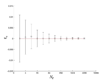
Figure 3: Convergence of $\epsilon_{u}$ as the number of ensemble measurements, $N_{e}$, is increased for a system governed by the Hamiltonian (24), characterized by perfect subspace confinement. The solid line represents the actual value of $\epsilon_{u}(H_{a})=0$. Note error bars should only extend to zero as $\epsilon_{u}(H_{a})\geq 0$.

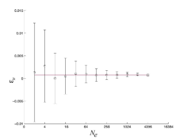
Figure 4: Convergence of $\epsilon_{u}$ as the number of ensemble measurements, $N_{e}$, is increased for the imperfectly confined system governed by the Hamiltonian (23). The solid line represents the actual value of $\epsilon_{u}(H_{b})\approx 7\times 10^{-4}$. Note error bars should only extend to zero as $\epsilon_{u}(H_{b})\geq 0$.

IV.2 Numerical tests of error bound accuracy

To test the overall accuracy of the uncertainty estimates for $\epsilon_{u}$ we can expect to obtain from realistic Rabi oscillation data, we calculated the distance between the simulated value, $\epsilon_{u}$, and the analytical value, $\epsilon_{u}^{\prime}$, calculated directly from the Hamiltonian using Eq. 15 as,

$$d(H_{k})=|\epsilon_{u}(H_{k})-\epsilon_{u}^{\prime}(H_{k})|,$$ (26)

where $k\in[a,b]$ and $\delta d(H_{k})$ is the error in $d$ resulting from the error associated with estimating $\epsilon_{u}(H_{k})$. We first calculated the distance $d(H_{k})$ and $\delta d(H_{k})$ for 5000 simulated runs of two known trial Hamiltonians ($H_{a}$ and $H_{b}$) with $\epsilon_{u}^{\prime}(H_{a})=0$ and $\epsilon_{u}^{\prime}(H_{b})\approx 7\times 10^{-4}$, respectively. The distributions of $d(H_{k})$ for $H_{a}$ and $H_{b}$ (with $N_{e}=1024$ and $t_{\rm ob}$ as in Figs 3 and 4 are shown in Figs 5 and 6, respectively. The average error $3\overline{\delta d(H_{i})}$, $i\in[a,b]$, was given by $3\overline{\delta d(H_{a})}\approx 4.92\times 10^{-4}$, encompassing $99.9\%$ of the data, and $3\overline{\delta d(H_{b})}\approx 5.02\times 10^{-4}$, encompassing $99.8\%$ of the data, respectively.

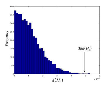
Figure 5: Distribution of $d(H_{a})$ for 5000 separate simulations. The average of the error, $3\overline{\delta d(H_{a})}$ is also shown, with approximately $99.9\%$ found within $3\sigma$ of $d=0$.

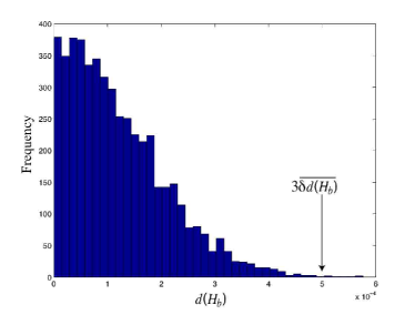
Figure 6: Distribution of $d(H_{b})$ for 5000 separate simulations. The average of the error, $3\overline{\delta d(H_{b})}$ is also shown, with approximately $99.8\%$ found within $3\sigma$ of $d=0$.

Next we examined how the protocol behaves when simulating a large number of randomly selected multi-level Hamiltonians. For these simulations we choose $N$-level Hamiltonians of the form

$$H_{N}=\sum_{k=0}^{9}E_{k}|k\rangle\langle k|+|0\rangle\langle 1|+\sum_{k=2}^{9}a_{k}|0\rangle\langle k|+\text{h.c.}$$ (27)

with $\{E_{k}\}\equiv\{0,1,1.5,2,2.4,2.5,2.9,3,3.3,4\}$. The vector $\vec{a}=[a_{2},\ldots,a_{9}]$ was then chosen at random in two stages. First the dimensionality of $\vec{a}$ is randomly selected, allowing the Hamiltonian to coherently drive any multi-level system, $N\in[2,3,..,10]$. The non-zero coupling values were then randomly assigned such that each element of $\vec{a}$ was approximately two orders of magnitude less than the qubit coupling term to ensure that all of the multi-level systems had high confinement.

We randomly generated 5000 of these Hamiltonians and $d(H_{k})=|\epsilon_{u}(H_{k})-\epsilon_{u}^{\prime}(H_{k})|$ was calculated. The average (analytical) value of $\epsilon_{u}^{\prime}(H_{k})$ for these 5000 trial Hamiltonians was found to be $\overline{\epsilon_{u}^{\prime}(H_{k})}=1.68\times 10^{-4}$. We then examined the ratio,

$$R=\frac{\text{Num}\{(d(H_{k})-3\delta d(H_{k})\leq 0)\}}{5000},$$ (28)

indicating the percentage of successful estimates of the subspace leakage within $3\sigma$. This ratio was calculated to be $R=99.9\%$, with the confinement estimates being outside the error bounds for only three of the randomly generated Hamiltonians.

These results are consistent with the expectation that approximately $99.7\%$ of the data should lie within $3\sigma$ of the mean and demonstrates that our methodology for characterizing subspace leakage can indeed be expected to yield accurate upper bounds on the subspace leakage in the vast majority of cases.

V Efficiency of the protocol

The protocol presented in the previous section allows us to determine quantitative bounds on the subspace leakage for imperfect qubits by determining only the main peaks in the Fourier spectrum. An alternative strategy is to try to identify all peaks in the Fourier spectrum. The presence of any peaks in addition to the two main peaks is indicative of subspace leakage and a quantitative estimate of the leakage rate can be obtained by determining the heights of the additional peaks. Both approaches have potential advantages and disadvantages. The former approach requires only the identification of the two main peaks but these need to be clearly resolved and the peak heights determined with high precision. The latter approach does not require precise estimates of peak heights but relies on the detection of additional peaks, which for high confinement will be much smaller than the major peaks, and are likely to be difficult to discriminate from the noise floor. This raises the question which strategy is more efficient to decide if the subspace leakage for a given qubit is below a certain error threshold.

To answer this question, we performed a series of numerical simulations comparing the total number of measurements required to ascertain that the lower bound on the leakage rate $\epsilon_{l}=1-\sqrt{h_{0}+2h_{0,1}}>0$ within error bounds, versus identifying a statistically significant third peak in the Fourier spectrum, indicating an out-of-subspace transition, for various trial Hamiltonians. For the purpose of the simulations we consider the following trial Hamiltonians

$$H_{3}=\begin{pmatrix}0&1&\gamma\\ 1&1&0\\ \gamma&0&1.5\end{pmatrix}$$ (29)

representing a system with a variable coupling $\gamma$ to a third level, as well as the four-level system governed by the Hamiltonian (21) and a six-level system governed by

$$H_{6}=\begin{pmatrix}0&1&\gamma&\gamma&\gamma&\gamma\\ 1&1&0&0&0&0\\ \gamma&0&1.5&0&0&0\\ \gamma&0&0&1.7&0&0\\ \gamma&0&0&0&1.9&0\\ \gamma&0&0&0&0&2.2\end{pmatrix},$$ (30)

representing systems with variable but equal coupling to between one and four out-of-subspace levels, respectively.

The lower bound, $\epsilon_{l}$, is taken to be non-zero for a discrete data set, if the analytical value $\epsilon^{\prime}_{l}$ of the lower bound calculated directly from the Hamiltonian exceeds six times the uncertainty, $\delta(\epsilon_{l})$, for the discrete data calculated from the simulated Fourier spectrum, i.e.,

$$\epsilon^{\prime}_{l}-6\delta(\epsilon_{l})>0,$$ (31)

$$\delta(\epsilon_{l})=\frac{3\delta h}{2\sqrt{h_{0}+2h_{0,1}}}.$$

Six times the uncertainty in $\epsilon_{\l}$ represents the total distance between the maximum and minimum possible value of $\epsilon_{l}$ (using a $3\sigma$ upper and lower confidence bound) and this interval should be smaller than the analytical value, $\epsilon^{\prime}_{l}$.

A peak $F(\omega^{\prime})$ in the discrete Fourier spectrum is taken to be significant if it is more than three standard deviations $\delta h=\text{sd}[\nu({\omega})]$ above the projection noise floor $\bar{\nu}(\omega)$, i.e.,

$$F(\omega^{\prime})-\bar{\nu}(\omega)-3\delta h>0.$$ (32)

This definition will underestimate the number of ensemble measurements required slightly as it only represents the point where the third peak is greater than at least 99.7% of the noise channels.

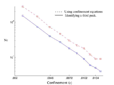
Figure 7: Number of ensemble measurements required to ascertain statistically significant subspace leakage (imperfect confinement) for the three-level system governed by (29) as a function of the (analytically calculated) confinement using the confinement equations (31) and by directly identifying the third transition peak.

For the simulations a range of out-of-subspace coupling strengths $\gamma$ was chosen for each of the trial Hamiltonians (29), (21) and (30), and the corresponding subspace leakage rate $\epsilon$ as well as the analytical lower bound $\epsilon_{l}^{\prime}$ computed. For each of the Hamiltonians we then simulated experimental Rabi data and computed the discrete Fourier spectrum. The observation time in all cases was 30 Rabi cycles and the number of ensemble measurements was $N_{e}=1024$. The number of ensemble measurements for the Rabi data simulations was gradually increased until a statistically significant third peak was found (32), or (31) was satisfied, respectively.

Fig. 7 shows the number of ensemble measurements $N_{e}$ necessary to conclude that the system is imperfect in the sense that leakage is statistically significant for the three-level system governed by (29) for both methods. The horizontal axis represents the analytical value of confinement $\epsilon(\gamma)$. Both curves scale roughly $1/\sqrt{N_{e}}$, which is consistent with the scaling of the projection noise, and hence the errors associated with estimating $\epsilon_{l}$ and detecting a statistically significant third peak. For the three-level system it is clear that confirming imperfect confinement by verifying (31) requires more ensemble measurements than detecting a third peak according to (32). This is not too surprising since for a three-level system there is only one additional transition $|0\rangle\leftrightarrow|2\rangle$, and from the derivations of the confinement equations (9) we have,

$$1 =\bigg{(}\sum_{a=0}^{N-1}|c_{a}|^{2}\bigg{)}^{2}$$ (33)

$$=\sum_{a=0}^{N-1}|c_{a}|^{4}+\sum_{a,b}|c_{a}|^{2}|c_{b}|^{2} =h_{0}+\sum_{a,b}h_{a,b},$$

i.e., there is a conservation law for the cumulative sum of all the peak heights. Hence, if the number of possible additional peaks is small, then for a given level of confinement, the additional peaks will be greater, and thus easier to detect, than for a system with weak coupling to a large number of out-of-subspace levels, and hence many small transition peaks. We therefore conjecture that estimating subspace leakage using (31) will become preferable for a system with coupling to multiple out-of-subspace levels. The results of numerical simulations for the Hamiltonians (21) and (30), shown in Fig 8 support this conjecture. We observe the same general scaling behavior as for the three-level system. For the four-level system it is clear that although searching for the additional transition peak is still somewhat more efficient, the difference between both methods is small. For the six-level the curves have swapped position, i.e., using the confinement equations has become a more efficient way to ascertain statistically significant subspace leakage.

In Appendix A we have included simulations for similar Hamiltonians up to ten levels to show the effective crossover of the curves and how the efficiency difference between the two methods increases with the number of additional levels. Note that for all the simulations we have endeavored to look at approximately the same range of subspace leakage. From these simulations it is clear that searching for the third peak in the Fourier spectrum is only really beneficial for systems with at most one extra transition. Hence, the proposed method for estimating subspace leakage will be more efficient than obvious alternatives in most cases.

VI The effect of Decoherence

It is well known that even if subspace leakage is theoretically suppressed for an arbitrary control field, it is unlikely that decoherence will also be suppressed. Hence, we need to examine if the proposed confinement protocol will still be effective in the open system case when a qubit is subject to decoherence, possibly of the same order, or greater, than subspace leakage.

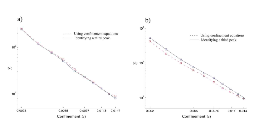
Figure 8: Number of ensemble measurements required to ascertain significant subspace leakage (imperfect confinement) for the four-level system governed by (21) [Fig. a] and the six-level system governed by (30) [Fig. b] using the confinement equations and identifying a third peak.

The study of arbitrary decoherence for $N$-level systems is a lengthy discussion, including Markovian and possible non-Markovian processes. Even for the simpler case of Markovian decoherence we would need to consider the complete $N$-level decoherence model with all the associated restrictions of completely positive maps sonia . Hence, we will instead only focus on a restricted case to show that, for a simple example, decoherence does not invalidate the protocol. It should be stressed that this only represents a preliminary analysis under a specific model of decoherence. Further work will involve investigating more complicated and system-specific decoherence effects such as $N$-level dephasing and spontaneous emission as well as possible system specific non-Markovian decoherence. However, due to the extremely complicated nature of such an analysis we will limit our discussion to a specific case.

We consider a perfectly confined qubit which undergoes Markovian decoherence and hence can be described by the quantum Liouville equation

$$\partial_{t}\rho=-\frac{i}{\hbar}[H,\rho]+\sum_{k=1}^{3}\Gamma_{k}\mathcal{L}_{k}[\rho]$$ (34)

where, $\mathcal{L}_{k}[\rho]=([L_{k},\rho L_{k}^{\dagger}]+[L_{k}\rho,L_{k}^{\dagger}])/2$, $H$ represents the single qubit control Hamiltonian, and $L_{k}$ are the Lindblad quantum jump operators, which describe the effect of the environment on the system, each parameterized by some rate $\Gamma_{k}\geq 0$.

For a basic decoherence analysis we restrict the Lindblad operators to the Pauli set, $\{L_{k}\}=\{X,Y,Z\}$, and consider a perfectly confined, control Hamiltonian of the form

$$H=\frac{d}{2}[\cos(\theta)Z+\sin(\theta)X].$$ (35)

This decoherence model is sufficient to describe pure dephasing as well as symmetric population relaxation processes in any basis, although not asymmetric relaxation processes. Including each Pauli Lindblad term with an associated decoherence rate eliminates the problem of a preferential basis for qubit decoherence since any basis change of the overall system will only act to change the form of the Hamiltonian.

We can solve the master equation under this model by using the Bloch vector formalism. Expressing the density matrix as $\rho(t)=I/2+x(t)X+y(t)Y+z(t)Z$, Eq. (34) takes the form $\partial_{t}S(t)=AS(t)$, where $S(t)=(x(t),y(t),z(t))^{T}$ and

$$A=\begin{pmatrix}-2(\Gamma_{y}+\Gamma_{z})&-d\cos(\theta)&0\\ d\cos(\theta)&-2(\Gamma_{x}+\Gamma_{z})&-d\sin(\theta)\\ 0&d\sin(\theta)&-2(\Gamma_{x}+\Gamma_{y})\end{pmatrix}.$$ (36)

The Rabi oscillations under this evolution are described by the function $f(t)=\text{Tr}[P_{0}\rho(t)]=(1/2)+z(t)$, where $P_{0}=|0\rangle\langle 0|$, with an initial state $\rho(0)=|0\rangle\langle 0|\implies S(0)=(0,0,1/2)^{T}$. Taking the Fourier transform of $f(t)$ leads to the rather complicated general expression (47) in Appendix B. The real component of this function describes three Lorentzians centered about $\omega=0$ and $\omega=\pm d$. Assuming that $d\gg\Gamma_{x,y,z}$, we can expand Eq. (47) around $\omega=0$ and $\omega=\pm d$ to obtain the functions [See Appendix B],

$$h_{0} =\frac{1}{2}\delta(\omega)+\frac{\cos^{2}(\theta)}{2}\frac{\Gamma_{\alpha}}{w^{2}+\Gamma_{\alpha}^{2}},$$ (37)

$$h_{0,1} =\frac{\sin^{2}(\theta)}{4}\frac{\Gamma_{\beta}}{(\omega\pm d)^{2}+\Gamma_{\beta}^{2}},$$

where $\Gamma_{\alpha}=2(\Gamma_{y}+\Gamma_{z}+\cos^{2}(\theta)(\Gamma_{x}-\Gamma_{z}))$, $\Gamma_{\beta}=\Gamma_{x}(1+\sin^{2}(\theta))+\Gamma_{y}+\Gamma_{z}(2-\sin^{2}(\theta))$ and $h_{0}$ contains a $\delta(\omega)$ offset due to the fact we are measuring the observable $P_{0}$. In order to describe how the maximum peak of each Lorentzian varies with $\Gamma$ we integrate $h_{0}$ and $h_{0,1}$ around an interval $\eta$ of the peak height

$$h_{0}(\eta) =\frac{\cos^{2}(\theta)}{2}\int_{-\eta}^{\eta}d\omega\frac{\Gamma_{\alpha}}{\omega^{2}+\Gamma_{\alpha}^{2}}+\frac{1}{2}\int_{-\eta}^{\eta}d\omega\delta(\omega)$$ (38)

$$=\frac{1}{2}+\frac{\cos^{2}(\theta)}{\pi}\arctan\bigg{(}\frac{\eta}{\Gamma_{\alpha}}\bigg{)},$$

$$h_{0,1}(\eta) =\frac{\sin^{2}(\theta)}{4}\int_{d-\eta}^{d+\eta}d\omega\frac{\Gamma_{\beta}}{(\omega-d)^{2}+\Gamma_{\beta}^{2}}$$

$$=\frac{\sin^{2}(\theta)}{2\pi}\arctan\bigg{(}\frac{\eta}{\Gamma_{\beta}}\bigg{)}.$$

Hence, under decoherence the peak heights in the Fourier spectrum vary as a function of the integration window $\eta$ and the decoherence rates $\Gamma_{\alpha,\beta}$. This is consistent since as $\Gamma_{\alpha,\beta}\rightarrow 0$, both $\arctan$ functions approach $\pi/2$ and $h_{0}+2h_{0,1}=1$. The integration window $\eta$ is analogous to frequency resolution of the Fourier transform $\Delta\omega$, while the total area of the Lorentzian is equal to the peak heights when $\Gamma_{x,y,z}=0$. Hence for small $\Gamma_{x,y,z}$ we can simply choose the resolution of the Fourier transform such that the entire Lorentzian is essentially contained within the data channel of the primary peak.

Consider the case where we wish to ensure that the subspace leakage does not exceed $\zeta$. Using the upper bound for the subspace leakage (15) we have, assuming that the integration interval is approximately equal to the frequency resolution of the DFT (i.e. $\eta\approx\Delta\omega$)

$$\zeta =\frac{1}{2}\bigg{(}1-\sqrt{2h_{0}(\Delta\omega)+4h_{0,1}(\Delta\omega)-1}\bigg{)},$$ (39)

$$\frac{(1-2\zeta)^{2}+1}{2} =\frac{1}{2}+\frac{\cos^{2}(\theta)}{\pi}\arctan\bigg{(}\frac{\Delta\omega}{\Gamma_{\alpha}}\bigg{)}$$

$$\quad\quad+\frac{\sin^{2}(\theta)}{\pi}\arctan\bigg{(}\frac{\Delta\omega}{\Gamma_{\beta}}\bigg{)}$$

$$\frac{\pi(1-2\zeta)^{2}}{2} =\arctan\bigg{(}\frac{\Delta\omega}{\Gamma}\bigg{)}.$$

Here the last line assumes that $\Gamma_{\alpha}\approx\Gamma_{\beta}=\Gamma$. When the Rabi frequency is much greater than the inverse of the decoherence rate (as necessary for any qubit realistically considered for quantum information processing), then the entire Lorentzian broadening caused by decoherence will be contained within one frequency channel. Thus, Eq. (39) allows us to calculate the maximum frequency resolution of the Fourier transform for successful leakage estimation using our protocol. For example, if $\Gamma\approx 10^{-4}\mathrm{s}^{-1}$ and we wish to confirm that the subspace leakage is at most $\epsilon_{\text{max}}=10^{-8}$, then the resolution of the Fourier transform cannot exceed $\Delta f\approx 250$Hz if only the primary peak channels are used. Obviously, this restriction on the frequency resolution can be lifted by including multiple channels around the central peak when estimating the peak area.

Although the decoherence model considered is not the most general possible case for an imperfectly confined control Hamiltonian, this calculation demonstrates that the effect of decoherence does not void the protocol for estimating subspace leakage for a common decoherence model. A more detailed analysis considering a full $N$-level decoherence model, including the effect of spontaneous emission and absorption processes and the possibility of system-specific non-Markovian decoherence is desirable but beyond the scope of the current paper.

VII Conclusions

We have introduced an intrinsic protocol for “quantifying” the degree of subspace leakage for a realistic ‘qubit’ system. The protocol relies on very minimal theoretical assumptions regarding qubit structure and control, and utilizes a measurement model that is restrictive but extremely common to a wide range of qubit systems. We have introduced a quantitative measure of subspace leakage, and shown that the discretization noise as a result of finite sampling does not limit the ability of the protocol to quantify (with appropriate error/confidence bounds) the subspace leakage for well-confined (near perfect) qubits.

The ability to experimentally characterize subspace leakage to a high degree of accuracy using automated, system independent methods, which rely on the intrinsic control and measurement apparatus of the quantum device (required for standard quantum information processing) will be vital for the commercial success of quantum nano-technology. This protocol represents one of the first steps in a general library of characterization techniques that will be required as “quality control” protocols once mass manufacturing of qubit systems becomes common.

Although, in this discussion, the qubit state $|1\rangle$ is only defined through the strongest transition it should be emphasized that if confinement estimates are made on multiple control fields (for example two separate Hamiltonians which induce orthogonal axis rotations), the computational $|1\rangle$ state must be common for both Hamiltonians. This is not a significant problem, since for well engineered qubits, the computational $|1\rangle$ state will be known on theoretical grounds.

There are many open problems including subspace leakage estimates for systems undergoing a whole range of potential decoherence processes, quantifying confinement for multi-qubit control Hamiltonians and combining these schemes with other proposed methods for system characterization. Hopefully, in the near future, a complete set of characterization protocols will be developed which will augment large scale manufacturing techniques, allowing for efficient and speedy transition of quantum technology from the physics laboratory to the commercial sector.

Appendix A Efficiency comparison for leakage detection protocols

The following simulations examined the minimal number of ensemble measurements required to detect imperfect qubits either via the confinement equations or by directly detecting the third transition peak. Three-level, four-level and six-level Hamiltonians are found in the main text, the additional simulations were performed for all other multi-level systems up to ten levels. The general form of each of the trial Hamiltonians are subsets of the ten-level system,

$$H_{10}=\sum_{k=0}^{9}E_{k}|k\rangle\langle k|+\gamma_{k}(|0\rangle\langle k|+|k\rangle\langle 0|)$$ (40)

where $\{E_{k}\}\equiv\{0,1,1.5,1.7,1.9,2.2,2.5,2.7,3,3.2\}$, $\gamma_{1}=1$ and $\gamma_{k}=\gamma$ for $k\neq 1$.

For each lower level system the appropriate Hamiltonian is simply formed by removing the appropriate number of rows and columns from $H_{10}$ (i.e. compare $H_{4}$ and $H_{6}$ in Eqs. (21) and (30)). Each of these systems were simulated leading to the following results [Figs 9, 10 and 11],

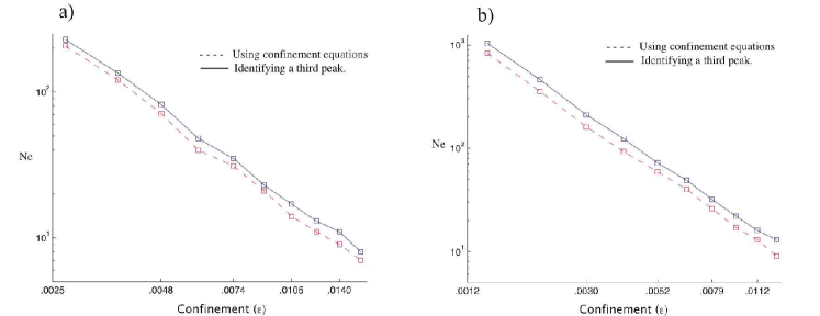
Figure 9: Number of ensemble measurements required to ascertain significant subspace leakage (imperfect confinement) for the five-level system [Fig. a] and the eight-level system [Fig. b] using the confinement equations and identifying a third peak.

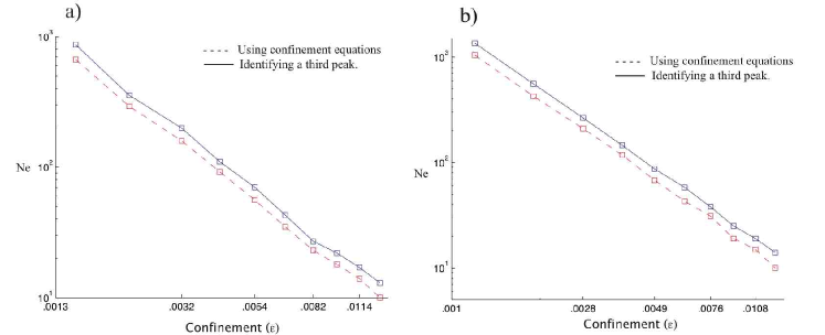
Figure 10: Number of ensemble measurements required to ascertain significant subspace leakage (imperfect confinement) for the seven-level system [Fig. a] and the nine-level system [Fig. b] using the confinement equations and identifying a third peak.

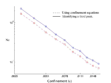
Figure 11: Number of ensemble measurements required to ascertain significant subspace leakage (imperfect confinement) for the ten-level system using the confinement equations and identifying a third peak.

Appendix B Solutions to the decoherence master equation

Here we show the derivations of Eq. 37 by solving the Bloch equation $\partial_{t}S(t)=AS(t)$, with $A$ given in Eq. (36). To solve this differential equation, we convert to Fourier space. Since the Fourier transform for a system governed by decoherence-induced semi-group dynamics is only defined for $t\geq 0$, we use the cosine and sine transforms

$$\mathcal{C}[f(t);\omega]=\int_{0}^{\infty}f(t)\cos(\omega t),$$ (41)

$$\mathcal{S}[f(t);\omega]=\int_{0}^{\infty}f(t)\sin(\omega t),$$

noting that

$$\mathcal{C}[f(t);\omega]-i\mathcal{S}[f(t);\omega]=\int_{0}^{\infty}f(t)e^{-i\omega t}=\mathcal{F}_{+}[f(t);\omega].$$ (42)

Taking the sine and cosine transforms of $\partial_{t}S(t)=AS(t)$, noting that

$$\mathcal{C}[\dot{f}(t);\omega]=\omega\mathcal{S}[f(t);\omega]-f(0),$$ (43)

$$\mathcal{S}[\dot{f}(t);\omega]=-\omega\mathcal{S}[f(t);\omega],$$

gives

$$\omega\mathcal{S}[S(t);\omega]-S(0)=A\mathcal{C}[S(t);w],$$ (44)

$$-\omega\mathcal{C}[S(t);\omega]=A\mathcal{S}[S(t);w].$$

Combining these equations and setting $S(\omega)=\mathcal{F}_{+}[S(t);\omega]$ yields,

$$i\omega S(\omega)-S(0)=AS(\omega),$$ (45)

and hence

$$S(\omega)=-(A-i\omega I)^{-1}S(0).$$ (46)

The initial condition $S(0)=(0,0,1/2)^{T}$ thus gives,

$$FT[z(t)]=-\frac{c^{2}d^{2}+(2\Gamma_{x}+2\Gamma_{z}+i\omega)(2\Gamma_{y}+2\Gamma_{z}+i\omega)}{2(c^{2}d^{2}+(2\Gamma_{x}+2\Gamma_{z}+i\omega)(2\Gamma_{y}+2\Gamma_{z}+i\omega))(-2(\Gamma_{x}+\Gamma_{y})-i\omega)-2d^{2}s^{2}(2\Gamma_{y}+2\Gamma_{z}+i\omega)},$$ (47)

where $c=\cos(\theta)$ and $s=\sin(\theta)$. The subsequent expansions are too lengthy to include here, however standard symbolic toolkits such as Mathematica can handle such expressions. The first step is to consider only the real component of $FT[z(t)]$. Next, the denominator is expanded to second order around $\omega=0$ or $\omega=\pm d$. After this, we expand the numerator and denominator, neglecting all terms of the form $\Gamma_{x,y,z}/d$ and smaller, assuming $\Gamma_{x,y,z}\ll d$ and being careful to note that for expansions around $\omega=\pm d$ we must keep terms of the form $\omega\Gamma_{x,y,z}/d$. After simplifying the expressions we find

$$h_{0} =\frac{\cos^{2}(\theta)}{2}\frac{\Gamma_{\alpha}}{w^{2}+\Gamma_{\alpha}^{2}},$$ (48)

$$h_{0,1} =\frac{\sin^{2}(\theta)}{4}\frac{\Gamma_{\beta}}{(\omega\pm d)^{2}+\Gamma_{\beta}^{2}},$$

where $\Gamma_{\alpha}=2(\Gamma_{y}+\Gamma_{z}+\cos^{2}(\theta)(\Gamma_{x}-\Gamma_{z}))$ and $\Gamma_{\beta}=\Gamma_{x}(1+\sin^{2}(\theta))+\Gamma_{y}+\Gamma_{z}(2-\sin^{2}(\theta))$. Confirming that Eq. (37) describes three Lorentzian curves centered on $\omega=0$ and $\omega=\pm d$.

- (1) J. E. Mooij, T.P. Orlando, L. Levitov, L. Tian, C.H. van der Wal and S. Lloyd, Science. 285, 1036-1039 (1999).
- (2) Y. Nakamura, C. D. Chen and J. S. Tsai, Nature (London). 398, 786 (1999).
- (3) M. R. Geller, E. J. Pritchett, A. T. Sornborger, F. K. Wilhelm, quant-ph/0603224 (2006).
- (4) M.D. Lukin and P.R. Hemmer, Phys. Rev. Lett. 84, 2818 (2000).
- (5) A.D. Greentree et. al., J. Phys: Condens. Matter. 18, (2006), S825-S842.
- (6) J. Wrachtrup, S. Y. Kilin and A.P. Nizovtsev, Optics and Spectroscopy. 91, 429-437 (2001).
- (7) J.I. Cirac and P. Zoller, Phys. Rev. Lett. 74, 4091 (1995).
- (8) J. Clarke et al., Science. 239, 992 (1988)
- (9) A. Blais, A. Maassen van den Brink and A. M. Zagoskin, Phys. Rev. Lett. 90, 127901 (2003).
- (10) A.M. Steane, Phys. Rev. Lett. 77, 793, (1996).
- (11) R. Laflamme, C. Miquel, J. P. Paz, and W. H. Zurek, Phys. Rev. Lett. 77, 198 (1996)
- (12) D. Gottesman, Ph.D Thesis (Caltech), quant-ph/9705052.
- (13) L.-A. Wu, M.S. Byrd and D.A. Lidar, Phys. Rev. Lett. 89, 127901 (2002).
- (14) M.S. Byrd, D. A. Lidar, L-A. Wu and P. Zanardi, Phys. Rev. A. 71, 052301 (2005).
- (15) R. Fazio, G. Palma and J. Siewert, Phys. Rev. Lett. 83, 5385 (1999).
- (16) C. Mochor, Phys. Rev. A. 69, 032306 (2004).
- (17) J. Preskill, Introduction to Quantum Computation, pages 213-269. World Scientific, Singapore, 1998.
- (18) M. Grassl, Th. Beth, T. Pellizzari, Phys. Rev. A. 56, 33 (1997).
- (19) J. Vala, K.B. Whaley and D.S. Weiss, Phys. Rev. A. 72, 052318 (2005).
- (20) K. Khodjasteh and D.A. Lidar, Phys. Rev. A. 68, 022322 (2003).
- (21) P. Aliferis, B.M. Terhal, Quant. Inf. Comp. 7, 139-156 (2006).
- (22) J.H. Cole et al., Phys. Rev. A. 71, 062312 (2005).
- (23) J.H. Cole, S.J. Devitt and L. C.L. Hollenberg, J. Phys. A: Math. Gen. 39, (2006), 14649-14658.
- (24) S.J. Devitt, J.H. Cole, L.C.L. Hollenberg, Phys. Rev. A. 73, 052317 (2006).
- (25) J.H. Cole et. al., Phys. Rev. A. 73, 062333 (2006).
- (26) M. H. Devoret and R. J. Schoelkopf, Nature (London). 406, 1039 (2000).
- (27) V. I. Conrad, A. D. Greentree, D. N. Jamieson and L. C.L. Hollenberg, J. Comput. Theor. Nanosci. 2, 214 (2005).
- (28) A. Aassime, G. Johansson, G. Wendin, R. J. Schoelkopf, and P. Delsing, Phys. Rev. Lett. 86, 3376 (2001).
- (29) J. M. Martinis, S. Nam, J. Aumentado and C. Urbina, Phys. Rev. Lett. 89, 117901 (2002).
- (30) G. Wendin and V. S. Shumeiko, cond-mat/0508729 (2005).
- (31) R. N. Bracewell, The Fourier transform and its applica- tions, McGraw-Hill series in electrical and computer en- gineering. Circuits and systems. (McGraw Hill, Boston, 2000), 3rd ed.14. (Clarendon Press, Oxford, 1990).
- (32) S.G. Schirmer and A.I. Solomon, Phys. Rev. A. 70, 022107 (2004).