Probing quantum phases of ultracold atoms in optical lattices by transmission spectra in cavity QED

Abstract

Studies of ultracold gases in optical lattices BlochNatPhys link many disciplines. They allow testing fundamental quantum many-body concepts of condensed-matter physics in well controllable atomic systems BlochNatPhys , e.g., strongly correlated phases, quantum information processing. Standard methods to observe quantum properties of Bose-Einstein condensates (BEC) are based on matter-wave interference between atoms released from traps BlochNature ; Lukin ; Stoferle ; Gritsev ; Schellekens , destroying the system. Here we propose a new, nondestructive in atom numbers, method based on optical measurements, proving that atomic quantum statistics can be mapped on transmission spectra of high-Q cavities, where atoms create a quantum refractive index. This can be extremely useful for studying phase transitions Jaksch , e.g. between Mott insulator and superfluid states, since various phases show qualitatively distinct light scattering. Joining the paradigms of cavity quantum electrodynamics (QED) and ultracold gases will enable conceptually new investigations of both light and matter at ultimate quantum levels. We predict effects accessible in experiments, which only recently became possible Esslinger .

All-optical methods to characterize atomic quantum statistics were proposed for homogeneous BEC You94 ; Jav94 ; You95 ; Jav95 ; Parkins and some modified spectral properties induced by BEC’s were attributed to collective emission You94 ; Jav94 , recoil shifts Jav95 or local field effects Morice .

We show a completely different phenomenon directly reflecting atom quantum statistics due to state-dependent dispersion. More precisely, the dispersion shift of a cavity mode depends on the atom number. If the atom number in some lattice region fluctuates from realization to realization, the modes get a fluctuating frequency shift. Thus, in the cavity transmission-spectrum, resonances appear at different frequencies directly reflecting the atom number distribution function. Such a measurement allows then to calculate atomic statistical quantities, e.g., mean value and variance reflected by spectral characteristics such as the central frequency and width.

Different phases of a degenerate gas possess similar mean-field densities but different quantum amplitudes. This leads to a superposition of different transmission spectra, which e.g. for a superfluid state (SF) consist of numerous peaks reflecting the discreteness of the matter-field. Analogous discrete spectra reversing the role of atoms and light, thus reflecting the photon structure of electromagnetic fields, were obtained in cavity QED with Rydberg atoms Haroche and solid-state superconducting circuits Schoelkopf . A quantum phase transition towards a Mott insulator state (MI) is characterized by a reduction of the number of peaks towards a single resonance, because atom number fluctuations are significantly suppressed Gerbier ; Campbell . As our detection scheme is based on nonresonant dispersive interaction independent of a particular level structure, it can be also applied to molecules Volz ; Winkler .

We consider the quantized motion of $N$ two-level atoms in a deep periodic optical lattice with $M$ sites formed by far off-resonance standing wave laser beams BlochNatPhys . A region of $K\leq M$ sites is coupled to two quantized light modes whose geometries (i.e. axis directions or wavelengths) can be varied. This is shown in Fig. 1 depicting two cavities crossed by a 1D string of atoms in equally separated wells generated by the lattice lasers (not shown). In practice two different modes of the same cavity would do as well.

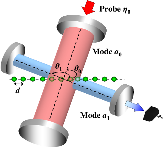
Figure 1: Schematic setup. Atoms are periodically trapped in an optical lattice created by laser beams, which are not shown in this figure. Additionally, the atoms are illuminated by two light modes at the angles $\theta_{0,1}$ with respect to the lattice axis.

As shown in the Methods section, the Heisenberg equations for the annihilation operators of two light modes $a_{l}$ ($l=0,1$) with eigenfrequencies $\omega_{l}$ and spatial mode functions $u_{l}({\bf r})$ are

$$\dot{a}_{l}=-i\left(\omega_{l}+\delta_{l}\hat{D}_{ll}\right)a_{l}-i\delta_{m}\hat{D}_{lm}a_{m}-\kappa a_{l}+\eta_{l}(t),$$ (1)

$$\text{with}\quad\hat{D}_{lm}\equiv\sum_{i=1}^{K}{u_{l}^{*}({\bf r}_{i})u_{m}({\bf r}_{i})\hat{n}_{i}},$$

where $l\neq m$, $\delta_{l}=g^{2}/\Delta_{la}$, $g$ is the atom-light coupling constant, $\Delta_{la}=\omega_{l}-\omega_{a}$ are the large cavity-atom detunings, $\kappa$ is the cavity relaxation rate, $\eta_{l}(t)=\eta_{l}e^{-i\omega_{lp}t}$ gives the external probe and $\hat{n}_{i}$ are the atom number operators at a site with coordinate ${\bf r}_{i}$. We also introduce the operator of the atom number at illuminated sites $\hat{N}_{K}=\sum_{i=1}^{K}{\hat{n}_{i}}$.

In a classical limit, Eq. (1) corresponds to Maxwell’s equations with the dispersion-induced frequency shifts of cavity modes $\delta_{l}\hat{D}_{ll}$ and the coupling coefficient between them $\delta_{1}\hat{D}_{10}$. For a quantum gas those quantities are operators, which will lead to striking results: atom number fluctuations will be directly reflected in such measurable frequency-dependent observables. Thus, cavity transmission-spectra will reflect atomic statistics.

Eq. (1) allows to express the light operators $a_{l}$ as a function $f(\hat{n}_{1},...,\hat{n}_{M})$ of atomic occupation number operators and calculate their expectation values for prescribed atomic states $|\Psi\rangle$. We start with the well known examples of MI and SF states and generalize to any $|\Psi\rangle$ later.

From the viewpoint of light scattering, the MI state behaves almost classically as, for negligible tunneling, precisely $\langle\hat{n}_{i}\rangle_{\text{MI}}=q_{i}$ atoms are well localized at the $i$th site with no number fluctuations. It is represented by a product of Fock states, i.e. $|\Psi\rangle_{\text{MI}}=\prod_{i=1}^{M}|q_{i}\rangle_{i}\equiv|q_{1},...,q_{M}\rangle$, with expectation values

$$\langle f(\hat{n}_{1},...,\hat{n}_{M})\rangle_{\text{MI}}=f(q_{1},...,q_{M}),$$ (2)

since $\hat{n}_{i}|q_{1},...,q_{M}\rangle=q_{i}|q_{1},...,q_{M}\rangle$. For simplicity we consider equal average densities $\langle\hat{n}_{i}\rangle_{\text{MI}}=N/M\equiv n$ ($\langle\hat{N}_{K}\rangle_{\text{MI}}=nK\equiv N_{K}$).

In our second example, SF state, each atom is delocalized over all sites leading to local number fluctuations at a lattice region with $K<M$ sites. Mathematically it is a superposition of Fock states corresponding to all possible distributions of $N$ atoms at $M$ sites: $|\Psi\rangle_{\text{SF}}=\sum_{q_{1},...,q_{M}}\sqrt{N!/M^{N}}/\sqrt{q_{1}!...q_{M}!}|q_{1},...,q_{M}\rangle$. Although its average density $\langle\hat{n}_{i}\rangle_{\text{SF}}=N/M$ is identical to a MI, it creates different light transmission spectra. Expectation values of light operators can be calculated from

$$\langle f(\hat{n}_{1},...,\hat{n}_{M})\rangle_{\text{SF}}=\frac{1}{M^{N}}\sum_{q_{1},...,q_{M}}\frac{N!}{q_{1}!...q_{M}!}f(q_{1},...,q_{M}),$$ (3)

representing a sum of all possible “classical” terms. Thus, all these distributions contribute to scattering from a SF, which is obviously different from $\langle f(\hat{n}_{1},...,\hat{n}_{M})\rangle_{\text{MI}}$ (2) with only a single contributing term.

In the simple case of only one mode $a_{0}$ ($a_{1}\equiv 0$), the stationary solution of Eq. (1) for the photon number reads

$$a^{\dagger}_{0}a_{0}=f(\hat{n}_{1},...,\hat{n}_{M})=\frac{|\eta_{0}|^{2}}{(\Delta_{p}-\delta_{0}\hat{D}_{00})^{2}+\kappa^{2}},$$ (4)

where $\Delta_{p}=\omega_{0p}-\omega_{0}$ is the probe-cavity detuning. We present transmission spectra in Fig. 2 for the case, where $|u_{0}({\bf r}_{i})|^{2}=1$, and $\hat{D}_{00}=\sum_{i=1}^{K}\hat{n}_{i}$ reduces to $\hat{N}_{K}$. For a 1D lattice (see Fig. 1), this occurs for a traveling wave at any angle, and standing wave transverse ($\theta_{0}=\pi/2$) or parallel ($\theta_{0}=0$) to the lattice with atoms trapped at field maxima.

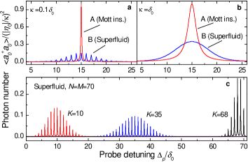
Figure 2: Photon number in a single cavity mode. a, Single Lorentzian for MI (curve A) reflects non-fluctuating atom number. Many Lorentzians for SF (curve B) reflect atom number fluctuations, which are imprinted on the positions of narrow resonances. Here $\kappa$ is smaller than satellite separation $\delta_{0}$ ($\kappa=0.1\delta_{0}$), $N=M=30$, $K=15$. b, The same as in a but $\kappa=\delta_{0}$ gives smooth broadened contour for SF. c, Spectra for SF with $N=M=70$ and different number of sites illuminated $K=10,35,68$. The transmission spectra have different forms, since different atom distribution functions correspond to different $K$. $\kappa=0.05\delta_{0}$.

For MI, the averaging of Eq. (4) according to Eq. (2) gives the photon number $\langle a^{\dagger}_{0}a_{0}\rangle_{\text{MI}}$, as a function of the detuning, as a single Lorentzian described by Eq. (4) with width $\kappa$ and frequency shift given by $\delta_{0}\langle\hat{D}_{00}\rangle_{\text{MI}}$ (equal to $\delta_{0}N_{K}$ in Fig. 2). Thus, for MI, the spectrum reproduces a simple classical result of a Lorentzian shifted due to dispersion.

In contrast, for a SF, the averaging procedure of Eq. (3) gives a sum of Lorentzians with different dispersion shifts corresponding to all atomic distributions $|q_{1},...,q_{K}\rangle$. So, if each Lorentzian is resolved, one can measure a comb-like structure by scanning the detuning $\Delta_{p}$. In Figs. 2a and 2c, different shifts of the Lorentzians correspond to different possible atom numbers at $K$ sites (which due to atom number fluctuations in SF, can take all values 0,1,2,…,$N$). The Lorentzians are separated by $\delta_{0}$. Thus, we see that atom number fluctuations lead to the fluctuating mode shift, and hence to multiple resonances in the spectrum. For larger $\kappa$ the spectrum becomes continuous (Fig. 2b), but broader than that for MI.

Scattering of weak fields does not change the atom number distribution. However, as the SF is a superposition of different atom numbers in a region with $K$ sites, a measurement projects the state into a subspace with fixed $N_{K}$ in this region, and a subsequent measurement on a time scale short to tunneling between sites will yield the same result. One recovers the full spectrum of Fig. 2 by repeating the experiment or with sufficient delay to allow for redistribution via tunneling. Such measurements will allow a time dependent study of tunneling and buildup of long-range order. Alternatively, one can continue measurements on the reduced subspace after changing a lattice region or light geometry.

We now consider two modes with $\omega_{0}=\omega_{1}$, the probe injected only into $a_{0}$ (Fig. 1) and the mentioned geometries where $\hat{D}_{00}=\hat{D}_{11}=\hat{N}_{K}$ (see Fig. 3). From Eq. (1), the stationary photon number $a^{\dagger}_{1}a_{1}=f(\hat{n}_{1},...,\hat{n}_{M})$ is

$$a^{\dagger}_{1}a_{1}=\frac{\delta_{1}^{2}\hat{D}^{\dagger}_{10}\hat{D}_{10}|\eta_{0}|^{2}}{[\hat{\Delta}^{\prime 2}_{p}-\delta_{1}^{2}\hat{D}^{\dagger}_{10}\hat{D}_{10}-\kappa^{2}]^{2}+4\kappa^{2}\hat{\Delta}^{\prime 2}_{p}},$$ (5)

where $\hat{\Delta}^{\prime}_{p}=\Delta_{p}-\delta_{1}\hat{D}_{11}$.

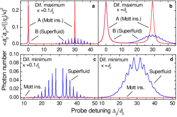
Figure 3: Photon number in one of two strongly coupled modes. a, Diffraction maximum, doublet for MI (curve A) and spectrum with structured right satellite for SF (curve B). Structure in the satellite reflects atom number fluctuations in SF, while narrow spectrum for MI demonstrates vanishing fluctuations. Here $\kappa$ is smaller than satellite separation $2\delta_{0}$ ($\kappa=0.1\delta_{0}$), $K=15$. b, The same as in a but $\kappa=\delta_{0}$ gives broadened satellite for SF. c, Diffraction minimum, zero field for MI and structured spectrum for SF. Nonzero structured spectrum for SF reflects fluctuating difference between atom numbers at odd and even sites, which exists even for the whole lattice illuminated, $K=M$. Here $\kappa$ is smaller than satellite separation $2\delta_{0}$ ($\kappa=0.1\delta_{0}$), $K=30$. d, The same as in c but $\kappa=\delta_{0}$ gives broadened contour for SF. $N=M=30$ in all figures.

In a classical (and MI) case, Eq. (2) gives a two-satellite contour (5) reflecting normal-mode splitting of two oscillators $\langle a_{0,1}\rangle$ coupled through atoms. This was recently observed Klinner for collective strong coupling, i.e., the splitting $\delta_{1}\langle\hat{D}_{10}\rangle$ exceeding $\kappa$. The splitting depends on the geometry (see Eq. (1)) representing diffraction of one mode into another. Thus, our results can be treated as scattering from a “quantum diffraction grating” generalizing Bragg scattering, well-known in different disciplines. In diffraction maxima (i.e. $u_{1}^{*}({\bf r}_{i})u_{0}({\bf r}_{i})=1$) one finds $\hat{D}_{10}=\hat{N}_{K}$ providing the maximal classical splitting. In diffraction minima, one finds $\hat{D}_{10}=\sum_{i=1}^{K}(-1)^{i+1}\hat{n}_{i}$ providing both the classical splitting and photon number are almost zero.

In SF, Eq. (3) shows that $\langle a^{\dagger}_{1}a_{1}\rangle_{\text{SF}}$ is given by a sum of all classical terms with all possible normal mode splittings. In a diffraction maximum (Figs. 3a,b), the right satellite is split into components corresponding to all possible $N_{K}$ or extremely broadened. In a minimum (Figs. 3c,d), the splittings are determined by all differences between atom numbers at odd and even sites $\sum_{i=1}^{K}(-1)^{i+1}q_{i}$. Note that there is no classical description of the spectra in a minimum, since here the classical field (and $\langle a^{\dagger}_{1}a_{1}\rangle_{\text{MI}}$) are simply zero for any $\Delta_{p}$. Thus, for two cavities coupled at diffraction minimum, the difference between the SF and MI states is even more striking: one has a structured spectrum instead of zero signal. Moreover, the difference between atom numbers at odd and even sites fluctuates even for the whole lattice illuminated, giving nontrivial spectra even for $K=M$.

In each of the examples in Figs. 2 and 3, the photon number depends only on one statistical quantity, now called $q$, $f(q_{1},...,q_{M})=f(q)$. For the single mode and two modes in a maximum, $q$ is the atom number at $K$ sites. For two modes in a minimum, $q$ is the atom number at odd (or even) sites. Therefore, expectation values for some state $|\Psi\rangle$ can be reduced to $\langle f\rangle_{\Psi}=\sum_{q=0}^{N}f(q)p_{\Psi}(q)$, where $p_{\Psi}(q)$ is the distribution function of $q$ in this state.

In high-Q cavities ($\kappa\ll\delta_{0}=g^{2}/\Delta_{0a}$), $f(q)$ is given by a narrow Lorentzian of width $\kappa$ peaked at some frequency proportional to $q$ ($q=0,1,...,N$). The Lorentzian hight is $q$-independent. Thus, $\langle f\rangle_{\Psi}$ as a function of $\Delta_{p}$ represents a comb of Lorentzians with the amplitudes simply proportional to $p_{\Psi}(q)$.

This is our central result. It states that the transmission spectrum of a high-Q cavity $\langle a^{\dagger}a(\Delta_{p})\rangle_{\Psi}$ directly maps the distribution function of ultracold atoms $p_{\Psi}(q)$, e.g., distribution function of atom number at $K$ sites. Various atomic statistical quantities characterizing a particular state can be then calculated: mean value (given by the spectrum center), variance (determined by the spectral width) and higher moments. Furthermore, transitions between different states will be reflected in spectral changes. Deviations from idealized MI and SF states Lewenstein are also measurable.

For SF, using $p_{\text{SF}}(q)$ (see Methods), we can write the envelopes of the comb of Lorentzians shown in Figs. 2a,c and 3a,c. As known, the atom number at $K$ sites fluctuates in SF with the variance $(\Delta N_{K})^{2}=N_{K}(1-K/M)$. For example, Fig. 2c shows spectra for different lattice regions demonstrating Gaussian and Poissonian distributions with the spectral width $\sigma_{\omega}=\delta_{0}\sqrt{(\Delta N_{K})^{2}}$, directly reflecting the atom distribution functions in SF. For $K\approx M$ the spectrum narrows, and, for the whole lattice illuminated, shrinks to a single Lorentzian as in MI.

The condition $\kappa<\delta_{0}=g^{2}/\Delta_{0a}$ is already met in present experiments. In the recent work Esslinger , where setups of cavity QED and ultracold gases were joined to probe quantum statistics of an atom laser with ⁸⁷Rb atoms, the parameters are $(g,\Delta_{0a},\kappa)=2\pi\times(10.4,30,1.4)$ MHz. The setups of cavity cooling Rempe ; Kimble are also very promising.

For bad cavities ($\kappa\gg\delta_{0}=g^{2}/\Delta_{0a}$), the sums can be replaced by integrals. The broad spectra in Figs. 2b and 3b,d are then given by convolutions of $p_{\Psi}(q)$ and Lorentzians. For example, curve B in Fig. 2b represents a Voigt contour, well-know in spectroscopy of hot gases. Here, the “inhomogeneous broadening” is a striking contribution of quantum statistics.

In summary, we exhibited that transmission spectra of cavities around a degenerate gas in an optical lattice are distinct for different quantum phases of even equal densities. Similar information is also contained in the field amplitudes $\langle a_{0,1}\rangle$ contrasting previous suggestions Parkins that $\langle a_{0,1}\rangle$ probes only the average density. This reflects (i) the orthogonality of Fock states corresponding to different atom distributions and (ii) the different frequency shifts of light fields entangled to those states. In general also other optical phenomena and quantities depending nonlinearly on atom number operators should similarly reflect the underlying quantum statistics We ; ICAP ; Meystre .

Methods

Derivation of Heisenberg equations

A manybody Hamiltonian for our system presented in Fig. 1 is given by

$$H=\sum_{l=0,1}\hbar{\omega_{l}a^{\dagger}_{l}a_{l}}+\int{d^{3}{\bf r}\Psi^{\dagger}({\bf r})H_{a1}\Psi({\bf r})},{\rm with}$$

$$H_{a1}=\frac{{\bf p}^{2}}{2m_{a}}+V_{\text{cl}}({\bf r})+\hbar g^{2}\sum_{l,m=0,1}{\frac{u_{l}^{*}({\bf r})u_{m}({\bf r})a^{\dagger}_{l}a_{m}}{\Delta_{ma}}},$$

where $a_{0,1}$ are the annihilation operators of the modes of frequencies $\omega_{0,1}$, wave vectors ${\bf k}_{0,1}$, and mode functions $u_{0,1}({\bf r})$; $\Psi({\bf r})$ is the atom-field operator. In the effective single-atom Hamiltonian $H_{a1}$, ${\bf p}$ and ${\bf r}$ are the momentum and position operators of an atom of mass $m_{a}$ trapped in the classical potential $V_{\text{cl}}({\bf r})$, and $g$ is the atom–light coupling constant. We consider off-resonant scattering where the detunings between fields and atomic transition $\Delta_{la}=\omega_{l}-\omega_{a}$ are larger than the spontaneous emission rate and Rabi frequencies. Thus, in $H_{a1}$ the adiabatic elimination of the upper state, assuming linear dipoles with adiabatically following polarization, was used.

For a one-dimensional lattice with period $d$ and atoms trapped at $x_{j}=jd$ ($j=1,2,\ldots,M$) the mode functions are $u_{0,1}({\bf r}_{j})=\exp(ijk_{0,1x}d+i\phi)$ for traveling and $u_{0,1}({\bf r}_{j})=\cos(jk_{0,1x}d+\phi)$ standing waves with $k_{0,1x}=|{\bf k}_{0,1}|\cos\theta_{0,1}$, $\theta_{0,1}$ are angles between the mode and lattice axes, $\phi$ is some spatial phase shift (cf. Fig. 1).

Assuming the modes $a_{0,1}$ much weaker than the trapping beam, we expand $\Psi({\bf r})$ using localized Wannier functions Jaksch corresponding to the potential $V_{\text{cl}}({\bf r})$ and keep only the lowest vibrational state at each site (we consider a quantum degenerate gas): $\Psi({\bf r})=\sum_{i=1}^{M}{b_{i}w({\bf r}-{\bf r}_{i})}$, where $b_{i}$ is the annihilation operator of an atom at site $i$ at a position ${\bf r}_{i}$. Substituting this expansion in the Hamiltonian $H$, one can get a generalized Bose-Hubbard model Jaksch including light scattering. In contrast to “Bragg spectroscopy”, which involves scattering of matter waves Stoferle , and our previous work Maschler , we neglect lattice excitations here and focus on light scattering from atoms in some prescribed quantum states.

Neglecting atomic tunneling, the Hamiltonian reads:

$$H=\sum_{l=0,1}{\hbar\omega_{l}a^{\dagger}_{l}a_{l}}+\hbar g^{2}\sum_{l,m=0,1}{\frac{a^{\dagger}_{l}a_{m}}{\Delta_{ma}}}\left(\sum_{i=1}^{K}{J_{i,i}^{lm}\hat{n}_{i}}\right),$$

where $\hat{n}_{i}=b_{i}^{\dagger}b_{i}$. For deep lattices the coefficients $J_{i,i}^{lm}=\int{d{\bf r}}w^{2}({\bf r}-{\bf r}_{i})u_{l}^{*}({\bf r})u_{m}({\bf r})$ reduce to $J_{i,i}^{lm}=u_{l}^{*}({\bf r}_{i})u_{m}({\bf r}_{i})$ neglecting spreading of atoms, which can be characterized even by classical scattering Slama . The Heisenberg equations obtained from this Hamiltonian are given by Eq. (1), were we have added a relaxation term. Strictly speaking, a Langevin noise term should be also added to Eq. (1). However, for typical conditions its influence on the expectation values of normal ordered field operators is negligible (see e.g. Davidovich ). In this paper, we are interested in the number of photons $\langle a_{l}^{\dagger}a_{l}\rangle$ only, which is a normal ordered quantity. Thus, one can simply omit the noise term in Eq. (1).

Simple expressions for spectral line shapes in SF state

We will now derive expressions for the spectra presented in Figs. 2 and 3 demonstrating relations between atomic quantum statistics and the transmission spectra for the SF state. As has been mentioned in the main text, in all examples presented in Figs. 2 and 3, the photon number depends only on a single statistical quantity, which we denote as $q$. Using this fact, the multinomial distribution in Eq. (3) reduces to a binomial, which can be directly derived from Eq. (3): $\langle f\rangle_{\text{SF}}=\sum_{q=0}^{N}f(q)p_{\text{SF}}(q)$ with $p_{\text{SF}}(q)=N!/[q!(N-q)!](Q/M)^{q}(1-Q/M)^{N-q}$ and a single sum instead of $M$ ones. Here $Q$ is the number of specified sites: $Q$ is equal to $K$ for one mode and two modes in a maximum; $Q$ is the number of odd (or even) sites for two modes in a minimum ($Q=M/2$ for even $M$). This approach can be used for other geometries, e.g., for two modes in a minimum and $K<M$, where Eq. (3) can be reduced to a trinomial distribution.

As a next approximation we consider $N,M\gg 1$, but finite $N/M$, leading to the Gaussian distribution $p_{\text{SF}}(q)=1/(\sqrt{2\pi}\sigma_{q})\exp{[-(q-\tilde{q})^{2}/2\sigma_{q}^{2}]}$ with central value $\tilde{q}=NQ/M$ and width $\sigma_{q}=\sqrt{N(Q/M)(1-Q/M)}$.

In high-Q cavities ($\kappa\ll\delta_{0}=g^{2}/\Delta_{0a}$), $f(q)$ is a narrow Lorentzian of width $\kappa$ peaked at some $q$-dependent frequency, now called $\Delta_{p}^{q}$. Since the Lorentzian hight is $q$-independent, $\langle f\rangle_{\text{SF}}$ as a function of $\Delta_{p}$ is a comb of Lorentzians with the amplitudes proportional to $p_{\text{SF}}(q)$.

Using the Gaussian distribution $p_{\text{SF}}(q)$,we can write the envelope of such a comb. For a single mode [Fig. 2a,c, Eq. (4)], we find $\Delta_{p}^{q}\approx\delta_{0}q$ with the envelope

$$\langle a_{0}^{\dagger}a_{0}(\Delta_{p}^{q})\rangle_{\text{SF}}=\frac{\alpha\delta_{0}}{\sqrt{2\pi}\sigma_{\omega}}e^{-(\Delta_{p}^{q}-\tilde{\Delta}_{p})^{2}/2\sigma_{\omega}^{2}},$$

where the central frequency $\tilde{\Delta}_{p}=\delta_{0}N_{K}$, spectral width $\sigma_{\omega}=\delta_{0}\sqrt{N_{K}(1-K/M)}$, and $\alpha=|\eta_{0}|^{2}/\kappa^{2}$. So, the spectrum envelopes in Fig. 2a,c are well described by Gaussians of widths strongly depending on $K$.

For $K\rightarrow 0$ and $K\rightarrow M$, the binomial distribution $p_{\text{SF}}(q)$ is well approximated by a Poissonian distribution, which is demonstrated in Fig. 2c for $K=10$ and $K=68$. For $K=M$ the spectrum shrinks to a single Lorenzian, since the total atom number at $M$ sites does not fluctuate.

In other examples (Figs. 3a and 3c), the above expression is also valid, although with other parameters. For two modes in a diffraction maximum (Fig. 3a), the central frequency, separation between Lorentzians and width are doubled: $\tilde{\Delta}_{p}=2\delta_{0}N_{K}$, $\Delta_{p}^{q}\approx 2\delta_{0}q$ and $\sigma_{\omega}=2\delta_{0}\sqrt{N_{K}(1-K/M)}$; $\alpha=|\eta_{0}|^{2}/(2\kappa^{2})$. The left satellite at $\Delta_{p}=0$ has a classical amplitude $|\eta_{0}|^{2}/(4\kappa^{2})$.

The nonclassical spectrum for two waves in a diffraction minimum (Fig. 3c) is centered at $\tilde{\Delta}_{p}=\delta_{0}N$, with components at $\Delta_{p}^{q}\approx 2\delta_{0}q$, and is very broad, $\sigma_{\omega}=\delta_{0}\sqrt{N}$; $\alpha=|\eta_{0}|^{2}/\kappa^{2}$.

For bad cavities ($\kappa\gg\delta_{0}$), the sums can be replaced by integrals with the same parameters $\tilde{\Delta}_{p}$ and $\sigma_{\omega}$ as for $\kappa<\delta_{0}$. For a single mode, Fig. 2b represents a Voigt contour

$$\langle a_{0}^{\dagger}a_{0}(\Delta_{p})\rangle_{\text{SF}}=\frac{|\eta_{0}|^{2}}{\sqrt{2\pi}\sigma_{\omega}}\int_{0}^{\infty}\frac{e^{-(\omega-\tilde{\Delta}_{p})^{2}/2\sigma_{\omega}^{2}}d\omega}{(\Delta_{p}-\omega)^{2}+\kappa^{2}}.$$

For two modes in a diffraction minimum the photon number (Fig. 3d) is

$$\langle a_{1}^{\dagger}a_{1}\rangle_{\text{SF}}=\frac{|\eta_{0}|^{2}}{\sqrt{2\pi}\sigma_{\omega}}\int_{-\infty}^{\infty}\frac{\omega^{2}e^{-\omega^{2}/2\sigma_{\omega}^{2}}d\omega}{(\Delta^{\prime 2}_{p}-\omega^{2}-\kappa^{2})^{2}+4\kappa^{2}\Delta^{\prime 2}_{p}},$$

where $\Delta^{\prime}_{p}=\Delta_{p}-\tilde{\Delta}_{p}$, while in a maximum (Fig. 3b)

$$\langle a_{1}^{\dagger}a_{1}\rangle_{\text{SF}}=\frac{|\eta_{0}|^{2}}{4\sqrt{2\pi}\sigma_{\omega}}\int_{0}^{\infty}\frac{\omega^{2}e^{-(\omega-\tilde{\Delta}_{p})^{2}/2\sigma_{\omega}^{2}}d\omega}{[\Delta_{p}(\Delta_{p}-\omega)+\kappa^{2}]^{2}+\kappa^{2}\omega^{2}}.$$

Competing financial interests

The authors declare that they have no competing financial interests.

References

- (1) Bloch, I. Ultracold quantum gases in optical lattices. Nat. Phys. 1, 23–30 (2005).
- (2) Fölling, S. et al. Spatial quantum noise interferometry in expanding ultracold atom clouds. Nature 434, 481–484 (2005).
- (3) Altman, E., Demler, E., & Lukin, M. D. Probing many-body states of ultracold atoms via noise correlations. Phys. Rev. A 70, 013603 (2004).
- (4) Stöferle, T., Moritz, H., Schori, C., Köhl, M. & Esslinger, T. Transition from a strongly interacting 1D superfluid to a Mott insulator. Phys. Rev. Lett. 92, 130403 (2004).
- (5) Gritsev, V., Altman, E., Demler, E. & Polkovnikov, A. Full quantum distribution of contrast in interference experiments between interacting one-dimensional Bose liquids. Nat. Phys. 2, 705–709 (2006).
- (6) Schellekens, M. et al. Hanbury Brown Twiss effect for ultracold quantum gases. Science 310, 648–651 (2005).
- (7) Jaksch, D., Bruder, C., Cirac, J. I., Gardiner, C. W. & Zoller, P. Cold bosonic atoms in optical lattices Phys. Rev. Lett. 81, 3108–3111 (1998).
- (8) Bourdel, T. et al. Cavity QED detection of interfering matter waves. Phys. Rev. A 73, 043602 (2006).
- (9) You, L., Lewenstein, M. & Cooper, J. Line shapes for light scattered from Bose-Einstein condensates. Phys. Rev. A 50, R3565–R3568 (1994).
- (10) Javanainen, J. Optical signatures of a tightly confined Bose condensate. Phys. Rev. Lett. 72, 2375–2378 (1994).
- (11) You, L., Lewenstein, M., & Cooper, J. Quantum field theory of atoms interacting with photons. II. Scattering of short laser pulses from trapped bosonic atoms. Phys. Rev. A 51, 4712–4727 (1995).
- (12) Javanainen, J. & Ruostekoski, J. Off-resonance light scattering from low-temperature Bose and Fermi gases. Phys. Rev. A 52, 3033–3046 (1995).
- (13) Parkins, A. S. & Walls, D. F. The physics of trapped dilute-gas Bose-Einstein condensates. Phys. Rep. 303, 1-80 (1998).
- (14) Morice, O., Castin, Y. & Dalibard, J. Refractive index of a dilute Bose gas. Phys. Rev. A 51, 3896–3901 (1995).
- (15) Brune, M., et al. Quantum Rabi oscillation: a direct test of field quantization in a cavity. Phys. Rev. Lett. 76, 1800–1803 (1996).
- (16) Gambetta, J. et al. Qubit-photon interactions in a cavity: Measurement-induced dephasing and number splitting. Phys. Rev. A 74, 042318 (2006).
- (17) Campbell, G. K. et al. Imaging the Mott insulator shells by using atomic clock shifts. Science 313, 649–652 (2006).
- (18) Gerbier, F., Fölling, S., Widera, A., Mandel, O. & Bloch, I. Probing number squeezing of ultracold atoms across the superfluid-Mott insulator transition. Phys. Rev. Lett. 96, 090401 (2006).
- (19) Volz, T. et al. Preparation of a quantum state with one molecule at each site of an optical lattice. Nat. Phys. 2, 692–695 (2006).
- (20) Winkler, K. et al. Repulsively bound atom pairs in an optical lattice. Nature 441, 853–856 (2006).
- (21) Klinner, J., Lindholdt, M., Nagorny, B. & Hemmerich, A. Normal mode splitting and mechanical effects of an optical lattice in a ring cavity. Phys. Rev. Lett. 96, 023002 (2006).
- (22) Lewenstein, M. et al. Ultracold atomic gases in optical lattices: Mimicking condensed matter physics and beyond. cond-mat/0606771.
- (23) Maunz, P. et al. Cavity cooling of a single atom. Nature 428, 50–52 (2004).
- (24) Hood, C. J., Lynn, T. W., Doherty, A. C., Parkins, A. S. & Kimble, H. J. The atom-cavity microscope: single atoms bound in orbit by single photons. Science 287, 1447–1453 (2000).
- (25) Mekhov, I. B., Maschler, C. & Ritsch, H. Cavity enhanced light scattering in optical lattices to probe atomic quantum satistics. quant-ph/0610073, Phys. Rev. Lett. 98, 100402 (2007); Mekhov, I. B., Maschler, C. & Ritsch, Light scattering from ultracold atoms in optical lattices as an optical probe of quantum statistics. quant-ph/0702193, Phys. Rev. A 76, 053618 (2007).
- (26) Mekhov, I. B., Maschler, C. & Ritsch, H., Light scattering from atoms in an optical lattice: optical probe of quantum statisticsin, Books of abstracts for the XX International Conference on Atomic Physics, ICAP, Innsbruck, 2006, p. 309 and conference web-site.
- (27) Chen, W., Meiser, D. & Meystre, P. Cavity QED determination of atomic number statistics in optical lattices. quant-ph/0610029.
- (28) Maschler, C. & Ritsch, H. Cold atom dynamics in a quantum optical lattice potential. Phys. Rev. Lett. 95, 260401 (2005); C. Maschler, I. B. Mekhov, and H. Ritsch. Ultracold atoms in optical lattices generated by quantized light fields. e-print arXiv:0710.4220.
- (29) Slama, S., von Cube, C., Kohler, M., Zimmermann, C. & Courteille, P. V. Multiple reflections and diffuse scattering in Bragg scattering at optical lattices. Phys. Rev. A 73, 023424 (2006).
- (30) Davidovich, L. Sub-Poissonian processes in quantum optics. Rev. Mod. Phys. 68, 127 (1996).