Strong-field spatial intensity-intensity correlations of light scattered from regular structures of atoms

Abstract

Photon correlations and cross-correlations of light scattered by a regular structure of strongly driven atoms are investigated. At strong driving, the scattered light separates into distinct spectral bands, such that each band can be treated as independent, thus extending the set of observables. We focus on second-order intensity-intensity correlation functions in two- and multi-atom systems. We demonstrate that for a single two-photon detector as, e.g., in lithography, increasing the driving field intensity leads to an increased spatial resolution of the second-order two-atom interference pattern. We show that the cross-correlations between photons emitted in the spectral sidebands violate Cauchy-Schwartz inequalities, and that their emission ordering cannot be predicted. Finally, the results are generalized for multi-particle structures, where we find results different from those in a Dicke-type sample.

I Introduction

Throughout the history of quantum physics, first-order correlations have played a major role in discussing the foundations of the underlying theory. One of the most famous model system is Young’s double-slit, which despite its simplicity allows to explore fundamental questions such as complementarity and uncertainty relations ficek ; uncert ; uncert2 ; uncert3 . A modern realization of Young’s experiment involves two atoms scattering near-resonant laser light eichmann ; mirror ; int1 ; int ; int2 ; int3 . The light is thus scattered by the simplest form of a regular structure, which gives rise to interference phenomena in the scattered light, because different indistinguishable pathways connect source and detector BornWolf . Analogous interference is also possible with single particles, demonstrating pathway interference in the energy-time domain otherschemes .

Starting with the experiments by Hanbury-Brown and Twiss hbt involving the measurement on a thermal field and the corresponding measurement with anti-bunched resonance fluorescence light antibunch , the second-order correlation function gained considerable attention. This correlation function measures intensity correlations and thus provides information on the fluctuation of the fields g2 .

In general, spatial interference in the different correlation functions can only be expected under certain experimental conditions. For example, it is possible to have interference in the second-order correlation function under conditions of no interference of the first-order correlation function int3 . In particular the first order interference in light scattered of regular structures of atoms is typically restricted to low incident light intensity and vanishes at strong driving int1 ; int ; int2 ; int3 ; cbs ; vogel ; letter . For example, in a two-particle system in the strong field limit, the collective dressed states are uniformly populated, and thus the interference fringe visibility is zero. Since applications often rely on these interference effects cbs ; vogel ; double-res ; letter , this restricts the potential implementation, where properties such as coherence, increased resolution, high signal-to-noise ratios or a rapid coherent system evolution are among the desirable properties of the scattered light.

More fundamentally, different lines of the frequency spectrum of the scattered light become separated in the strong-field limit, just as in the Mollow resonance fluorescence spectrum of a single strongly-driven two-level atom. We have shown recently that this separation can be employed to recover full first-order interference fringe visibility in the strong-field limit, and to gain a clearer interpretation and an extended set of observables to describe the scattered light letter . The basic idea was to facilitate a frequency-dependent electromagnetic bath, which can be realized, for example, using cavities or photonic crystals Cexp ; John . The focus of this work, however, was on first-order correlation functions.

Here, we discuss spatial second-order quantum interference effects in strong driving fields. As in the strong-field limit the spectral lines are well-separated, we define observables for each of the spectral lines separately. This allows for additional observables such as cross-correlations between different the spectral lines. First, we investigate the spatial dependence of the second-order correlation functions for a strongly driven atomic pair in free space and focus on the case of a single two-photon detector registering photons at the driving laser frequency $\omega_{L}$, as, for example, in lithography with a medium sensitive to two-photon exposure. We show that in this setup, the spatial resolution of the central strong-field second-order interference pattern can be increased by a factor of two as compared to the corresponding weak-field pattern simply by increasing the driving field intensity. This allows to create structures with high spatial resolution and signal intensity. Next, quantum cross-correlations between photons emitted in different spectral bands are investigated. In particular, we show that the spatial Cauchy-Schwarz inequalities (CSI) are violated for photons emitted into the sideband spectral lines over a wide range of detector positions. Also, it is impossible to predict the temporal ordering of two photons emitted in different sidebands. Our scheme can be realized in a wide range of systems, and can also be employed to analyze the structure of the scatterers. Finally, we generalize our results to the case of a linear chain of $N$ atoms, where the results are found to be different from results in Dicke-type samples.

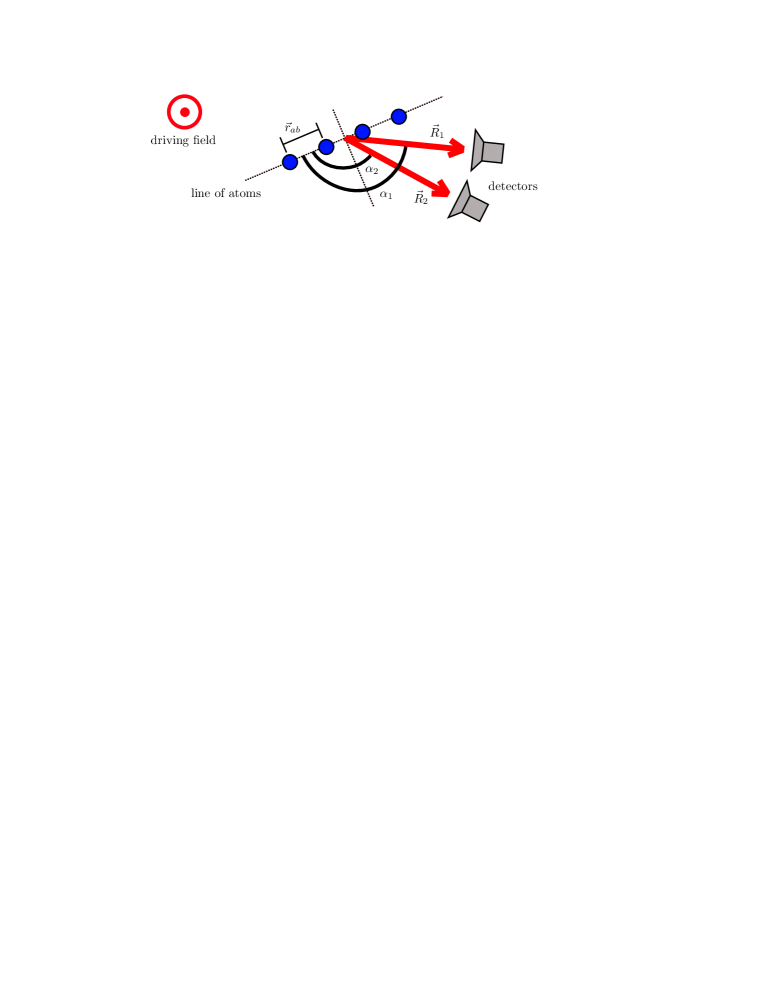
Figure 1: A linear structure of two-state emitters, where neighboring atoms are separated by the distance vectors $\vec{r}_{ab}$. The whole structure is driven by a resonant strong external laser field with wave vector $\vec{k}_{L}$. The two detectors are used to measure correlations among the photons emitted in observation directions $\vec{R}_{1},\vec{R}_{2}$, which are also characterized by the angles $\alpha_{1},\alpha_{2}$ between $\vec{r}_{ab}$ and $\vec{R}_{1},\vec{R}_{2}$. The line of atoms and the two detectors are located in a plane, and the driving field propagates perpendicular to this plane.

II Analytical treatment

We first concentrate on a driven pair of distinguishable non-overlapping two-state emitters, labeled $a$ and $b$, and generalize the discussion to a linear structure of $N>2$ atoms in section V. The two atoms both have atomic transition frequency $\omega_{0}$, are located at positions $\vec{r}_{a}$, $\vec{r}_{b}$, and are separated by $\vec{r}_{ab}$. The electronic bare ground state of atom $j\in\{a,b\}$ is labeled by $|1\rangle_{j}$, the corresponding excited state is $|2\rangle_{j}$. The external driving field with frequency $\omega_{L}=ck_{L}$ and wave vector $\vec{k}_{L}$ is aligned such that $\vec{k}_{L}\cdot\vec{r}_{ab}=0$ (see Fig. 1). The particles are spontaneously damped via the interaction with the surrounding electromagnetic field (EMF) reservoir. Our aim is to investigate the spatial photon correlations of the light scattered by the atoms in the intense driving field limit.

Assuming the electric dipole and rotating wave approximations, the laser-dressed atomic system is described by the Hamiltonian $H$ = $H_{0}$ + $H_{I}$, with

$$H_{0} =\sum_{k}\hbar(\omega_{k}-\omega_{L})a^{\dagger}_{k}a_{k}+\sum_{j\in\{a,b\}}\hbar\tilde{\Omega}R_{zj},\allowdisplaybreaks[2]$$ (1)

$$H_{I} =i\sum_{k}\sum_{j\in\{a,b\}}(\vec{g}_{k}\cdot\vec{d}_{j})\left\{a^{\dagger}_{k}\left(R_{zj}\frac{\sin{2\theta}}{2}-R^{(j)}_{21}\sin^{2}{\theta}+R^{(j)}_{12}\cos^{2}{\theta}\right)e^{-i(\vec{k}-\vec{k}_{L})\cdot\vec{r}_{j}}-\textrm{H.c.}\right\}.$$ (2)

Here, $H_{0}$ is the Hamiltonian of the free EMF and the free dressed atomic subsystems, while $H_{I}$ describes the interaction of the laser-dressed atoms with the EMF. $a_{k}$ and $a^{\dagger}_{k}$ are the radiation field annihilation and creation operators obeying the commutation relations $[a_{k},a^{\dagger}_{k^{{}^{\prime}}}]=\delta_{kk^{{}^{\prime}}}$, and $[a_{k},a_{k^{{}^{\prime}}}]$= $[a^{\dagger}_{k},a^{\dagger}_{k^{{}^{\prime}}}]=0$. The atomic operators $R^{(j)}_{\alpha\beta}=|\tilde{\alpha}\rangle_{j}{}_{j}\langle\tilde{\beta}|$ describe the transitions between the dressed states $|\tilde{\beta}\rangle_{j}$ and $|\tilde{\alpha}\rangle_{j}$ in atom $j$ for $\alpha\not=\beta$ and dressed-state populations for $\alpha=\beta$, and satisfy the commutation relation

$$[R^{(j)}_{\alpha\beta},R^{(l)}_{\alpha^{{}^{\prime}}\beta^{{}^{\prime}}}]=\delta_{jl}\left[\delta_{\beta\alpha^{{}^{\prime}}}R^{(j)}_{\alpha\beta^{{}^{\prime}}}-\delta_{\beta^{{}^{\prime}}\alpha}R^{(j)}_{\alpha^{{}^{\prime}}\beta}\right]\,.$$ (3)

The operators $R^{(j)}_{\alpha\beta}$ can be represented through the bare state operators via the transformations

$$|1\rangle_{j}=\sin{\theta}|\tilde{2}\rangle_{j}+\cos{\theta}|\tilde{1}\rangle_{j}\,,\qquad|2\rangle_{j}=\cos{\theta}|\tilde{2}\rangle_{j}-\sin{\theta}|\tilde{1}\rangle_{j}\,,$$ (4)

where the mixing angle $\theta$ is given by $\cot{2\theta}=\Delta/(2\Omega)$. The laser field detuning is $\Delta=\omega_{0}-\omega_{L}$, and the Rabi frequency is defined by $2\Omega=(\vec{d}\cdot\vec{E}_{L})/\hbar$. Here, $E_{L}$ is the electric laser field strength, and $\vec{d}\equiv\vec{d}_{a}=\vec{d}_{b}$ is the transition dipole matrix element. We further define the population inversion operators $R_{zj}=|\tilde{2}\rangle_{j}{}_{j}\langle\tilde{2}|-|\tilde{1}\rangle_{j}{}_{j}\langle\tilde{1}|$ and the generalized Rabi frequency $\tilde{\Omega}=[\Omega^{2}+(\Delta/2)^{2}]^{1/2}$. The dressed state transition frequencies are $\omega_{L},\omega_{\pm}=\omega_{L}\pm 2\tilde{\Omega}$. The two-particle spontaneous decay and the vacuum-mediated collective interactions are given by the frequency-dependent expression

$$\gamma_{jl}(\omega)=\gamma(\omega)[\chi_{jl}(\omega)+i\Omega_{jl}(\omega)]\,.$$ (5)

Independent of the atom-vacuum coupling, the collective parameters $\chi_{jl}$ and $\Omega_{jl}$ ($j\neq l$) tend to zero in the large-distance case $r_{jl}\to\infty$ which corresponds to the absence of coupling among the emitters. In the small-distance case $r_{jl}\to 0$, the parameter $\chi_{jl}$ tends to unity, while $\gamma\Omega_{jl}$ tends to the static dipole-dipole interaction potential.

In the intense field limit $\tilde{\Omega}\gg N\gamma$, different lines of the spectrum are well-separated. This allows us to investigate the spatial dependence of the second - order correlation functions for each of the spectral band separately. In this case, it follows from the interaction Hamiltonian Eq. (2) that the operators

$$R_{zj}\sin{2\theta}/2,\qquad R^{(j)}_{21}\cos^{2}\theta\qquad{\rm and}~{}~{}R^{(j)}_{12}\sin^{2}\theta$$ (6)

can be considered as the sources of the $m$th spectral field components $\{m\in C,R,L\}$. Here, $C$ stands for the central spectral band emitted at frequency $\omega_{L}$, and $R$ and $L$ are for the right and left sidebands emitted at frequencies $\omega_{L}+2\tilde{\Omega}$ and $\omega_{L}-2\tilde{\Omega}$, respectively KL . In the following, we use this decomposition to investigate the spatial properties of the photon statistics and cross-correlations between photons emitted from different spectral lines.

III Two-particle quantum dynamics

In order to be able to derive analytic expressions for the required expectation values, we first investigate the two-atom quantum dynamics in a strongly driven laser field. We introduce, for this reason, the two-atom collective dressed states as

$$|\Psi_{e}\rangle=|\tilde{2}_{a},\tilde{2}_{b}\rangle\,,\quad|\Psi_{s(a)}\rangle=\frac{1}{\sqrt{2}}(|\tilde{2}_{a},\tilde{1}_{b}\rangle\pm|\tilde{2}_{b},\tilde{1}_{a}\rangle)\,,\quad\textrm{ and }|\Psi_{g}\rangle=|\tilde{1}_{a},\tilde{1}_{b}\rangle\,.$$ (7)

The variables $\sigma_{\alpha\beta}=\langle|\Psi_{\alpha}\rangle\langle\Psi_{\beta}|\rangle$ are expectation values of the corresponding transition ($\alpha\not=\beta$) and population operators ($\alpha=\beta$) $(\{\alpha,\beta\}\in\{e,s,a,g\})$. Using Eqs. (1,2), one can obtain the equations of motion for the dressed-state variable of interest, i.e., $x=2(\sigma_{ee}-\sigma_{gg})$, $y=\sigma_{ss}-\sigma_{aa}$, and $z=\sigma_{ee}+\sigma_{gg}-\sigma_{ss}-\sigma_{aa}$, as mario :

$$\dot{x}(t) =-2\xi^{(+)}x+4\zeta^{(-)}_{ab}y+4\xi^{(-)}\,,\allowdisplaybreaks[2]$$ (8a)

$$\dot{y}(t) =-\zeta^{(-)}_{ab}x-2(c^{(0)}_{ab}+\xi^{(+)})y+2\zeta^{(+)}_{ab}z\,,\allowdisplaybreaks[2]$$ (8b)

$$\dot{z}(t) =2\xi^{(-)}x+4\zeta^{(+)}_{ab}y-4\xi^{(+)}z\,.$$ (8c)

The coefficients in these equations are defined as

$$\xi^{(\pm)} =\gamma(\omega_{-})\sin^{4}{\theta}\pm\gamma(\omega_{+})\cos^{4}{\theta}\,,$$ (9a)

$$\zeta^{(\pm)}_{ab} =\gamma(\omega_{-})\chi_{ab}(\omega_{-})\sin^{4}{\theta}\pm\gamma(\omega_{+})\chi_{ab}(\omega_{+})\cos^{4}{\theta}\,,$$ (9b)

$$c^{(0)}_{ab} =\gamma(\omega_{L})[1-\chi_{ab}(\omega_{L})]\sin^{2}{2\theta}\,.$$ (9c)

Simple analytical expressions for the two-atom steady-state quantum dynamics can be obtained if the two-particle interaction is mediated by the usual vacuum modes of the environmental electromagnetic reservoir, i.e. $\gamma(\omega_{-})$ = $\gamma(\omega_{+})$ = $\gamma(\omega_{L})\equiv\gamma$. Then, one obtains that

$$x=2\xi^{(-)}/\xi^{(+)},\quad y=0,\quad{\rm and}~{}~{}z=[\xi^{(-)}/\xi^{(+)}]^{2}.$$ (10)

In this case, the diagonal atomic dynamics is independent of the inter-atomic separation providing that $\Omega\gg\{\gamma\Omega_{ab},N\gamma\}$. In particular for $\theta=\pi/4$, i.e., exact resonance, we find that $x=y=z=0$, which means that the single-atom dressed states are equally populated.

IV Second-order correlation functions and two-particle side-band photon correlations

We now turn to the second-order correlation function of the steady-state resonance fluorescence emitted in the three spectral bands. The coherence properties of an electromagnetic field, at space-point $\vec{R}$, can be evaluated with the help of the second-order coherence functions:

$$g^{(2)}_{mn}(\tau,\vec{R}_{1},\vec{R}_{2})=\frac{\langle a^{+}_{m}(t,\vec{R}_{1})\,a^{+}_{n}(t+\tau,\vec{R}_{2})\,a_{n}(t+\tau,\vec{R}_{2})\,a_{m}(t,\vec{R}_{1})\rangle}{\langle a^{+}_{m}(t,\vec{R}_{1})\,a_{m}(t,\vec{R}_{1})\rangle\>\langle a^{+}_{n}(t,\vec{R}_{2})\,a_{n}(t,\vec{R}_{2})\rangle},$$ (11)

where $a_{n}^{+}~{}(a_{n})$ are the photon creation (annihilation) operator for modes $n\in\{C,L,R\}$. The quantity $g^{(2)}_{mn}(\tau)$ can be interpreted as a measure for the probability for detecting one photon emitted in mode $m$ and another photon emitted in mode $n$ with delay $\tau$. From now on, all correlation functions are evaluated for $\tau=0$, and, for notational simplicity, we drop the variable $\tau$. We further define two Cauchy-Schwarz parameters

$$\chi_{L}(\vec{R}_{1},\vec{R}_{2})=\frac{g^{(2)}_{LL}(\vec{R}_{1},\vec{R}_{2})g^{(2)}_{RR}(\vec{R}_{1},\vec{R}_{2})}{[g^{(2)}_{LR}(\vec{R}_{1},R_{2})]^{2}}\,,\quad\chi_{R}(\vec{R}_{1},\vec{R}_{2})=\frac{g^{(2)}_{LL}(\vec{R}_{1},\vec{R}_{2})g^{(2)}_{RR}(\vec{R}_{1},\vec{R}_{2})}{[g^{(2)}_{RL}(\vec{R}_{1},R_{2})]^{2}}\,,$$ (12)

which relate the correlation between photons emitted into individual modes to the cross-correlation between photons emitted into two different modes. If $\chi_{L}<1$ or $\chi_{R}<1$, the respective Cauchy-Schwarz inequalities are violated CSI .

We now turn to detection in the far-zone limit, and specialize to a resonant driving field ($\theta=\pi/4$). Then the field operators $a_{n}^{+}~{}(a_{n})$ entering in $g^{(2)}_{mn}$ and corresponding, respectively, to the three spectral modes of the Mollow spectrum can be represented via the atomic operators given in Eq. (6). With the help of Eqs. (1-10), and in Born-Markov and secular approximation, one arrives at the following expressions for the two-particle photon-correlations:

$$g^{(2)}_{CC}(\vec{R}_{1},\vec{R}_{2}) = 1+\cos{\delta_{1}}\cos{\delta_{2}}\,,$$ (13a)

$$g^{(2)}_{LL}(\vec{R}_{1},\vec{R}_{2}) = g^{(2)}_{RR}(\vec{R}_{1},\vec{R}_{2})=\frac{1}{2}[1+\cos(\delta_{1}-\delta_{2})]\,,$$ (13b)

$$g^{(2)}_{LR}(\vec{R}_{1},\vec{R}_{2}) = g^{(2)}_{RL}(\vec{R}_{1},\vec{R}_{2})=\frac{1}{2}[3+\cos(\delta_{1}+\delta_{2})]\,,$$ (13c)

$$g^{(2)}_{CX}(\vec{R}_{1},\vec{R}_{2}) = g^{(2)}_{XC}(\vec{R}_{1},\vec{R}_{2})=1\qquad\textrm{ for }X\in\{L,R\}\,.$$ (13d)

Here we used that in the resonant strong-field limit one has $\langle R_{zj}\rangle_{s}=\langle R^{(j)}_{12}\rangle_{s}=\langle R^{(j)}_{21}\rangle_{s}=0$ and $\langle R_{zi}R_{zj}\rangle_{s}=\langle R^{(i)}_{21}R^{(j)}_{12}\rangle_{s}=0$, where $i\not=j\in\{a,b\}$ denote one of the two atoms. The parameters $\delta_{d}$ ($d\in\{1,2\}$) are related to the detection angles $\alpha_{d}$ by $\delta_{d}=k\,r_{ab}\,\cos\alpha_{d}$, where we have assumed a planar geometry of atomic sample and observation detections.

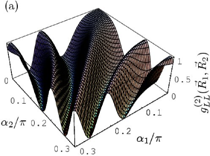
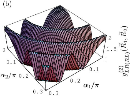
Figure 2: (a) Second-order side-band photon correlations $g_{LL(RR)}^{(2)}(\vec{R}_{1},\vec{R}_{2})$ and (b) cross-correlations $g_{LR(RL)}^{(2)}(\vec{R}_{1},\vec{R}_{2})$ as function of the detector positions $\alpha_{1},\alpha_{2}$. The interatomic distance is $r_{ab}/\lambda=5$, and the number of atoms is $N=2$.

Already the structure of Eqs. (13) reveals interesting insight in the nature of the light emitted in the various spectral bands. From the properties of the $\cos$ function it follows that $0\leq g^{(2)}_{CC}(\vec{R}_{1},\vec{R}_{2})\leq 2$, and $0\leq g^{(2)}_{LL}(\vec{R}_{1},\vec{R}_{2})=g^{(2)}_{RR}(\vec{R}_{1},\vec{R}_{2})\leq 1$, and $1\leq g^{(2)}_{LR}(\vec{R}_{1},\vec{R}_{2})=g^{(2)}_{RL}(\vec{R}_{1},\vec{R}_{2})\leq 2$. The cross-correlations involving the central spectral band are always unity and do not exhibit a dependence on the detection position. This immediately fixes the possible photon statistics of the emitted light. We observe a tendency to have pairs of photons emitted in the central band or pairs where one of the photons is in either sideband (left and right). In general, for these correlation functions, values below unity denote sub-poissonian light statistics, a value of units indicates poissonian statistics, and values above unity stand for super-poissonian light statistics.

An example for the second-order sideband photon correlation functions $g_{LL}^{(2)}$ and $g_{RR}^{(2)}$ as a function of the detection angles $\delta_{1},\delta_{2}$ is shown in Fig. 2(a). The spatial interference fringes of the second-order correlation function are clearly visible, and the range of possible values for $g_{LL}^{(2)}$ and $g_{RR}^{(2)}$ shows that both poissonian and sub-poissonian photon statistics can be generated at the sideband frequencies. Fig. 2(b) shows the corresponding results for the second-order cross-correlations $g_{LR}^{(2)}$ and $g_{RL}^{(2)}$. Here, the oscillatory structure is different, and values from 1 to 2 are obtained for the cross-correlations. Therefore poissonian as well as super-poissonian light statistics can be generated in the cross-correlations. In general, sub-Poissonian and Poissonian light statistics can be generated in all three spectral lines, and super-Poissonian light statistics is possible in the central spectral band second-order correlation function $g_{CC}^{(2)}$ and in the cross-correlations, see, e.g., Eq. (13).

We now discuss the second-order spatial interference of the light emitted in the central frequency band around $\omega_{L}$ for a specific detection scheme. We assume identical detection angles $\delta_{1}=\delta_{2}\equiv\delta$ and detection positions $\vec{R}_{1}=\vec{R}_{2}\equiv\vec{R}$, which corresponds, e.g., to a medium sensitive to two-photon exposure double-res . In the following, we discuss the interference fringe resolution of this setup, which is of relevance to applications in lithography, where the general aim is to create structures as small as possible. In the strong-field limit $\Omega/\gamma\gg 1$, from Eq. (13) we find $g^{(2)}_{CC}(\vec{R})=1+\cos^{2}{\delta}$. In the weak field case $\Omega/\gamma<1$ without spectral band separation, however, one finds $g^{(2)}(\vec{R})=[s/(s+\cos{\delta})]^{2}$ with $s=1+2(\Omega/\gamma)^{2}$ int2 . Comparing these two results, one finds that simply increasing the driving field strength effectively doubles the spatial fringe resolution in this setup around the central frequency $\omega_{L}$.

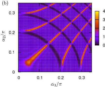
Figure 3: The Cauchy-Schwarz parameter $\chi_{L}=\chi_{R}$ as function of detector positions $\alpha_{1},\alpha_{2}$. Here, $r_{ab}/\lambda=5$. The number of atoms is (a) $N=2$ and (b) $N=8$.

After the discussion of the central spectral band, we now turn to the sideband frequencies around $\omega_{L}\pm 2\Omega$. Again, we consider detection in the far zone limit, but at this time the two detectors are at different positions. Under this conditions, the Cauchy-Schwarz parameters in Eq. (12) evaluate to

$$\chi_{L}=\chi_{R}=\biggl{[}\frac{1+\cos(\delta_{1}-\delta_{2})}{3+\cos(\delta_{1}+\delta_{2})}\biggr{]}^{2}.$$ (14)

This results is shown in Fig. 3(a) for an interparticle distance $r_{ab}=5\lambda$ and two atoms ($N=2$). One may easily observe that for a large range of detector positions $\delta_{1},\delta_{2}$, the Cauchy-Schwarz inequalities are violated, i.e., $\chi_{L}=\chi_{R}<1$. These results for $\chi_{L}$ and $\chi_{R}$ can be easily understood by inspecting Eq. (12) and Fig. 2. The Cauchy-Schwarz parameters are given by the ratio of the product of the sideband second-order photon correlations $g^{(2)}_{LL}(\vec{R})$ and $g^{(2)}_{RR}(\vec{R})$ to the cross correlation $g^{(2)}_{LR}(\vec{R})$ or $g^{(2)}_{RL}(\vec{R})$ squared. Therefore, both oscillatory structures in Fig. 2 are combined to give the result in Fig. 3(a). It is interesting to note that it is not possible to distinguish whether the first photon is emitted on the left or on the right sideband, since the two different cross-correlations $g^{(2)}_{LR}(\vec{R})$ and $g^{(2)}_{RL}(\vec{R})$ are equal.

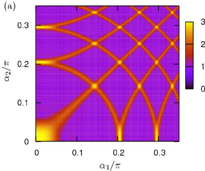
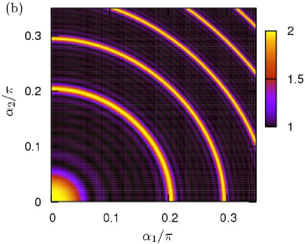
Figure 4: (a) Second-order side-band photon correlations $g_{CC}^{(2)}(\vec{R}_{1},\vec{R}_{2})$ and (b) $g_{LR}^{(2)}(\vec{R}_{1},\vec{R}_{2})=g_{RL}^{(2)}(\vec{R}_{1},\vec{R}_{2})$ as function of the detector positions $\alpha_{1},\alpha_{2}$. The interatomic distance is $r_{ab}/\lambda=5$, and the number of atoms is $N=8$.

V Multi-particle structures

In this final part, we discuss the case of $N$ independent two-level emitters that are uniformly distributed in a regular chain. Thus the inter-particle separations between the neighbor particles is assumed uniform and equal to $r_{0}$. As before, the atoms are driven by a strong laser field, $\Omega/\gamma\gg 1$. We further assume detection in the far-zone limit, that is, the linear dimension of the chain $L=(N-1)r_{0}$ is much smaller than the distances between chain and detectors $|\vec{R}_{1}|$ and $|\vec{R}_{2}|$. Then the second-order correlation functions for the light emitted in the central- and the sidebands as well as to the cross-correlations can be evaluated to give

$$g^{(2)}_{CC}(\vec{R}_{1},\vec{R}_{2}) = 1-\frac{2}{N}+\frac{1}{N^{2}}[\phi(\delta_{1}+\delta_{2})+\phi(\delta_{1}-\delta_{2})]\,,$$ (15a)

$$g^{(2)}_{LL}(\vec{R}_{1},\vec{R}_{2}) = g^{(2)}_{RR}(\vec{R}_{1},\vec{R}_{2})=1-\frac{2}{N}+\frac{1}{N^{2}}\phi(\delta_{1}-\delta_{2})\,,$$ (15b)

$$g^{(2)}_{LR}(\vec{R}_{1},\vec{R}_{2}) = g^{(2)}_{RL}(\vec{R}_{1},\vec{R}_{2})=1+\frac{1}{N^{2}}\phi(\delta_{1}+\delta_{2})\,,$$ (15c)

$$g^{(2)}_{CX}(\vec{R}_{1},\vec{R}_{2}) = g^{(2)}_{XC}(\vec{R}_{1},\vec{R}_{2})=1\qquad\textrm{ for }X\in\{L,R\}\,,$$ (15d)

where $\phi(\delta)=\sin^{2}(N\delta/2)/\sin^{2}(\delta/2)$.

In the multi-particle case, the Cauchy-Schwarz parameters Eq. (12) for the side-band photon correlations are given by the following expression

$$\chi_{L}=\chi_{R}=\biggl{[}\frac{N^{2}-2N+\phi(\delta_{1}-\delta_{2})}{N^{2}+\phi(\delta_{1}+\delta_{2})}\biggr{]}^{2}.$$ (16)

Figure 3(b) shows this Cauchy-Schwarz parameter for a linear chain of $N=8$ atoms. In this figure, the Cauchy-Schwarz parameters assume values from below unity up to 4. In the following, we discuss two special cases to demonstrate this more clearly. First, consider a two-photon detector with $\delta_{1}=\delta_{2}\equiv\delta$. Then Eq. (16) reduces to

$$\chi_{L}=\chi_{R}=\left(\frac{2N(N-1)}{N^{2}+\phi(2\delta)}\right)^{2}$$ (17)

which for $N\gg 1$ and $\delta=n\pi~{}(n=0,1,\cdots)$ tends to $\chi_{L(R)}\to 1$ while for $\delta=\pi(1+2n)/2$ we have $\chi_{L(R)}\to 4$. If, for instance, $\delta_{1}(\delta_{2})=0$ and $\delta_{2}(\delta_{1})\equiv\delta$ with $N\gg 1$ then $\chi_{L(R)}$ goes to unity as $\chi_{L(R)}=[1-1/N]^{2}$ when $\delta=n\pi~{}(n=0,1,\cdots)$ and to $\chi_{L(R)}=[1-2/N]^{2}$ for $\delta=\pi(1+2n)/2$. Thus, violation of CSI is likely to occur for moderate atomic structures.

Fig. 4(a) shows the central band second order correlation function $g^{(2)}_{CC}(\vec{R}_{1},\vec{R}_{2})$ for $N=8$ atoms versus the detection angles $\alpha_{1},\alpha_{2}$. Comparing this figure with Fig. 3(b), it is apparent that the dark regions in Fig. 3(b) that correspond to a super-poissonian photon emission statistics for a pair of photons from the left and the right spectral sideband [see Fig. 4(b)] are regions of high correlation in Fig. 4(a) as well. Thus, in these detection directions, super-poissonian statistics is observed in the central spectral band and the cross-correlations of the sideband photons.

Finally we note that the properties of the correlation functions found here are quite different from those obtained in a Dicke-type sample CS_B ; dicke2 ; CS_mek . For example, Dicke-type samples do not exhibit the spatial dependence originating from the regular structure discussed here, since the Dicke model involves the assumption that all atoms interact with the electromagnetic fields with the same phase. In particular, the first-order correlation function in our present model is linear in the number of atoms $N$, whereas it is proportional to the number of atoms squared in the Dicke model. The unnormalized second-order correlation function is proportional to $N^{4}$ and does not depend on the detection direction in Dicke-type samples. For regular structures, the unnormalized second-order correlation function depends at most on $N^{2}$ for particular detection positions. This detector position dependence arises from the geometrical phase factors $\exp(i\vec{k}\cdot\vec{r}_{ab})$, and not from collectivity. Constructive interfere of these phase factors gives rise to the dependence on $N^{2}$ for particular observation directions.

VI Summary and Conclusion

In summary, the intensity-intensity correlations of photons scattered by a strongly pumped linear atomic structure was investigated in detail. For this, the spectrum of the scattered light was separated into different spectral bands which we treated independently. In the central band at the driving laser field frequency, the resonant two-particle second-order interference fringes for two-photon detection have double resolution in the strong-field case as compared to the weak-field pattern. We found violation of the spatial Cauchy-Schwarz inequalities for photons emitted into the spectral sidebands, and that it is impossible to predict which photon is emitted first. Multiparticle atomic structures significantly enhance the intensity of the emitted correlated photons, and exhibit properties different from those in Dicke-type multiparticle samples.

References

- (1) Z. Ficek and S. Swain, Quantum Interference and Coherence: Theory and Experiments (Springer, Berlin, 2005).
- (2) N. Bohr, in Albert Einstein: Philosopher-Scientist, edited by P. A. Schilpp (Library of Living Philosophers, Evanston, 1949), pp. 200-241; reprinted in Quantum Theory and Measurement, edited by J. A. Wheeler and W. H. Zurek (Princeton University Press, Princeton, 1983), pp. 8-49.
- (3) M. O. Scully, B.-G. Englert, and H.Walther, Nature 351, 111 (1991); P. Storey, S. Tan, M. Collet, and D. Walls, Nature 367, 626 (1994); B.-G. Englert, M. O. Scully, and H.Walther, Nature 375, 367 (1995); E. P. Storey, S. M. Tan, M. J. Collet, and D. F. Walls, Nature 375, 368 (1995); H. Wiseman and F. Harrison, Nature 377, 584 (1995); H. M. Wiseman, F. E. Harrison, M. J. Collet, S. M. Tan, D. F.Walls, and R. B. Killip, Phys. Rev. A 56, 55 (1997).
- (4) S. Dürr, T. Nonn, and G. Rempe, Nature 395, 33 (1998); A. Luis and L. L. Sanchez-Soto, J. Opt. B: Quantum Semiclass. Opt. 1, 668 (1999).
- (5) U. Eichmann et al., Phys. Rev. Lett. 70, 2359 (1993).
- (6) J. Eschner et al., Nature (London) 413, 495 (2001).
- (7) G. S. Agarwal, J. von Zanthier, C. Skornia, and H. Walther, Phys. Rev. A 65, 053826 (2002).
- (8) T. Richter, Opt. Commun. 80, 285 (1991); P. Kochan et al., Phys. Rev. Lett. 75, 45 (1995); G. M. Meyer and G. Yeoman, ibid 79, 2650 (1997); T. Wong et al., Phys. Rev. A 55, 1288 (1997); W. H. Itano et al., ibid 57, 4176 (1998); T. Rudolph and Z. Ficek, ibid 58, 748 (1998); G. Yeoman, ibid 58, 764 (1998); Ch. Schön and Almut Beige, ibid 64, 023806 (2001).
- (9) M. Wiegand, J. Phys. B: At. Mol. Phys. 16, 1133 (1983).
- (10) C. Skornia et al., Phys. Rev. A 64, 063801 (2001).
- (11) M. Born and E. Wolf, Principles of optics (CUP, Cambridge, 1999).
- (12) F. Lindner et al., Phys. Rev. Lett. 95, 040401 (2005), and references therein; M. Kiffner, J. Evers and C. H. Keitel, Phys. Rev. Lett. 96, 100403 (2006).
- (13) R. Hanbury-Brown and R. Q. Twiss, Nature 177, 27 (1956).
- (14) H. J. Kimble, M. Dagenais, and L. Mandel, Phys. Rev. Lett. 39, 691 (1977).
- (15) C. W. Gardiner, Quantum Noise (Springer, Berlin, 1991); J. Perina, Quantum statistics of linear and nonlinear optical phenomena (Kluwer, Dordrecht, 1984).
- (16) V. Shatokhin et al., Phys. Rev. Lett. 94, 043603 (2005).
- (17) W. Vogel and D.-G. Welsch, Phys. Rev. Lett. 54, 1802 (1985).
- (18) M. Macovei, J. Evers, G.-x. Li, and C. H. Keitel, Phys. Rev. Lett. 98, 043602 (2007).
- (19) A. N. Boto et al., Phys. Rev. Lett. 85, 2733 (2000); M. D’Angelo, M. V. Chekhova and Y. Shih, ibid. 87, 013602 (2001); J. Xiong et al., ibid. 94, 173601 (2005); P. R. Hemmer et al., ibid 96, 163603 (2006); C. H. Keitel and S. X. Hu, Appl. Phys. Lett. 80, 541 (2002).
- (20) Y. Zhu et al., Phys. Rev. Lett. 61, 1946 (1988); A. Lezama et al., Phys. Rev. A 39, R2754 (1989).
- (21) M. Florescu and S. John, Phys. Rev. A 69, 053810 (2004).
- (22) P. A. Apanasevich, S. J. Kilin, J. Phys. B: At. Mol. Phys. 12, L83 (1979).
- (23) M. Dal Col, M. Macovei, and C. H. Keitel, Opt. Commun. 264, 407 (2006).
- (24) R. Loudon, Rep. Prog. Phys. 43, 58 (1980); M. S. Zubairy, Phys. Lett. A 87, 162 (1982).
- (25) N. N. Bogolubov Jr., A. S. Shumovsky, and Tran Quang, Phys. Lett. A 123, 71 (1987).
- (26) N. N. Bogolubov, Jr. et al., J. Phys. B: At. Mol. Phys. 20, 1885 (1987).
- (27) M. Macovei, J. Evers, and C. H. Keitel, Phys. Rev. A. 72, 063809 (2005).