A Quantum Algorithm for the Hamiltonian NAND Tree

Abstract

We give a quantum algorithm for the binary NAND tree problem in the Hamiltonian oracle model. The algorithm uses a continuous time quantum walk with a run time proportional to $\sqrt{N}$. We also show a lower bound of $\sqrt{N}$ for the NAND tree problem in the Hamiltonian oracle model. MIT-CTP/3813

1 Introduction

The NAND trees in this paper are perfectly bifurcating trees with N leaves at the top and depth $n=\log_{2}(N)$. Each leaf is assigned a value of 0 or 1 and the value of any other node is the NAND of the two connected nodes just above. The goal is to evaluate the value at the root of the tree. An example is shown in figure (1). Classically there is a randomized algorithm that succeeds after evaluating only (with high probability) $N^{.753}$ of the leaves. This algorithm is known to be best possible. See [4] and references there.

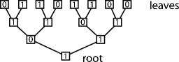
Figure 1: A classical NAND tree.

As far as we know, no quantum algorithm has been devised which improves on the classical query complexity. However there is a quantum lower bound of $\sqrt{N}$ calls to a quantum oracle [4]. In this paper we are not working in the usual quantum query model but rather with a Hamiltonian oracle [1, 3] which encodes the NAND tree instance. We will present a quantum algorithm which evaluates the NAND tree in a running time proportional to $\sqrt{N}$. We also prove a lower bound of $\sqrt{N}$ on the running time for any quantum algorithm in the Hamiltonian oracle model.

Our quantum algorithm uses a continuous time quantum walk on a graph [5]. We start with a perfectly bifurcating tree of depth n and one additional node for each of the N leaves. To specify the input we connect some of these N pairs of nodes. A connection corresponds to an input value of 1 on a leaf in the classical NAND tree and the absence of a connection corresponds to a 0. See the top of figure (2). Next we attach a long line of nodes to the root of the tree. We call this long line the “runway”. See the bottom of figure (2). The Hamiltonian for the continuous time quantum walk we use here is minus the adjacency matrix of the graph. As usual with continuous time quantum walks, nodes in the graph correspond to computational basis states.

Figure 2: The full Hamiltonian $H_{O}+H_{D}$

We can decompose this Hamiltonian into an oracle, $H_{O}$, which is instance dependent and a driver, $H_{D}$, which is instance independent. $H_{D}$ is minus the adjacency matrix of the perfectly bifurcating tree of depth n whose root is attached to node 0 of the line of nodes running from $-M$ to $M$. We will take $M$ to be very large. See figure (3).

Figure 3: The oracle independent driver Hamiltonian $H_{D}$

$H_{O}$ is minus the adjacency matrix of a graph consisting of the leaves of the bifurcating tree and the parallel set of N other nodes. Each leaf in the tree is connected or not to its corresponding node in the set above. See figure (4). The quantum problem is: Given the Hamiltonian oracle $H_{O}$, evaluate the NAND tree with the corresponding input.

Figure 4: The Hamiltonian oracle $H_{O}$

Our quantum algorithm evolves with the full Hamiltonian $H_{O}+H_{D}$, which is minus the adjacency matrix of the full graph illustrated in figure (2). The initial state is a carefully chosen right moving packet of length L localized totally on the left side of the runway with the right edge of the packet at node $0$. It will turn out that $L$ is of order $\sqrt{N}$. We take M to be much larger than $L$, say of order $L^{2}$. We now let the quantum system evolve and wait a time $L/2$ which is the time it would take this packet to move a distance $L$ to the right if the tree were not present. We then measure the projector onto the subspace corresponding to the right side of the runway. If the quantum state is found on the right we evaluate the NAND tree to be 1 and if the quantum state is not on the right we evaluate the NAND tree to be 0.

We have chosen our right moving packet to be very narrowly peaked in energy around $E=0$. (Note that $E=0$ is not the ground state but is the middle of the spectrum.) The narrowness of the packet in energy forces the packet to be long. If we did not attach the bifurcating tree at node 0, the packet would just move to the right and we would find it on the right when we measure. The algorithm works because with the tree attached the transmission coefficient at $E=0$ is 0 if the NAND tree evaluates to 0 and the transmission coefficient at $E=0$ is 1 if the NAND tree evaluates to 1. The transmission coefficient is a rapidly changing function of $E$ but for $|E|<1/(16\sqrt{N})$ the transmission coefficient is not far from its value at $E=0$. To guarantee that the packet consists mostly of energy eigenstates with their energies in this range, we take $L$ to be of order $\sqrt{N}$. This determines the $\sqrt{N}$ run time of the algorithm.

Our algorithm uses the driver Hamiltonian $H_{D}$ to evaluate the NAND tree. An arbitrary algorithm can add any instance independent $H_{A}\,(t)$ to $H_{O}$ and work in the associated Hilbert space. We will show that for any choice of instance independent $H_{A}\,(t)$ the running time required to evaluate the NAND tree associated with $H_{O}$ is of order at least $\sqrt{N}$.

2 Motion on the Runway

Here we describe the evolution of a quantum state initially localized on the left side of the runway in figure (2) headed to the right. M is so large that we can take it to be infinite as is justified by the fact that the speed of propagation is bounded. First consider the infinite runway with integers $r$ labeling the sites. The tree is attached at $r=0$. We then have for all $r$ not equal to 0:

$$H\,|r\rangle=-|r+1\rangle-|r-1\rangle\qquad r\neq 0.$$ (2.1)

For $\theta>0,e^{ir\theta}$ and $e^{-ir\theta}$ correspond to the same energy (nonnormalized) eigenstate of equation (2.1) with energy

$$E(\theta)=-2\,\cos\,\theta$$ (2.2)

but the first is a right moving wave and the second is a left moving wave. We are interested in a packet, that is, a spatially finite superposition of energy eigenstates, which is incident from the left on the node 0 and the attached tree. This packet will scatter back and also transmit to the right side of the runway. The packet is dominated by energy eigenstates, $|E\rangle$, of the form on the runway

$$\langle r|E\rangle =\left[e^{ir\theta}+R(E)\,e^{-ir\theta}\right] \quad\mbox{for}\ r\leq 0,$$ (2.3)

$$\langle r|E\rangle =T(E)e^{ir\theta} \quad\mbox{for}\ r\geq 0.$$ (2.4)

(The states $|E\rangle$ do not vanish in the tree.) There are other energy eigenstates, but we will not need them. Furthermore from standard scattering theory we have

$$\langle E(\theta)|E(\theta^{\prime})\rangle=2\pi\delta(\theta-\theta^{\prime}).$$ (2.5)

Looking at $r=0$ we see that

$$1+R\,(E)=T\,(E).$$ (2.6)

The transmission coefficient $T(E)$ is determined by the structure of the tree. In particular let

$$y\,(E)=\frac{\langle\mbox{root}|E\rangle}{\langle r=0|E\rangle}$$ (2.7)

where “root” is the node immediately above $r=0$ on the runway, see figure (2). Applying the Hamiltonian at $|r=0\rangle$ gives

$$H|r=0\rangle=-|r=-1\rangle-|r=1\rangle-|\mbox{root}\rangle$$ (2.8)

and taking the inner product with $|E\rangle$ gives

$$T(E)=\frac{2\,i\,\sin\theta}{2\,i\,\sin\theta+y\,(E)}\ .$$ (2.9)

In the next section we will show how to calculate $y(E)$ and show that if the NAND tree evaluates to 1 then $y(0)=0$ meaning that $T(0)=1$ and if the NAND tree evaluates to 0 then $y(0)=\infty$ and $T(0)=0$. Unfortunately we cannot build a state with only E=0 since it would be infinitely long. Instead we build a finite packet that is long enough so that it is effectively a superposition of the states $|E\rangle$ with $E$ close enough to $0$ that $T(E)$ is close to $T(0)$. We introduce two parameters $\varepsilon$ and $D$ for which

$$|T(E)-T(0)|<D|E|\quad\mbox{for}\quad|E|<\varepsilon\,.$$ (2.10)

The parameters $\varepsilon$ and $D$ do depend on the size of the tree, but for the remainder of this section we only use $\varepsilon\ll 1$ and $\varepsilon D\ll 1$.

The initial state we consider, $|\psi(0)\rangle$, is given on the runway as

$$\langle r|\psi(0)\rangle = \frac{1}{\sqrt{L}}\ e^{ir\pi/2}\qquad\mbox{for}\qquad-L+1\leq r\leq 0$$ (2.11)

$$= 0\qquad\hskip 41.91672pt\mbox{for}\qquad r\leq-L\quad\mbox{and}\quad r>0$$

and vanishes in the tree. For this state

$$\langle\psi(0)|H|\psi(0)\rangle=0$$ (2.12)

and

$$\langle\psi(0)|H^{2}|\psi(0)\rangle=\frac{5}{L}$$ (2.13)

so the spread in energy about $0$ is of order $1/\sqrt{L}$. However, for our purpose we will see that this state is effectively more narrowly peaked in energy, and (2.13) is really an artifact of its sharp edge. In fact most of the probability in energy is contained in a peak around 0 of width $1/L$. Because we take $\pi/2$ and not $-\pi/2$ in (2.11) we have a right moving packet with energies near 0.

Evolving with the full Hamiltonian of the graph we have

$$|\psi(t)\rangle=e^{-iHt}|\psi{(0)}\rangle.$$ (2.14)

We decompose $|\psi(t)\rangle$ into two orthogonal parts,

$$|\psi(t)\rangle=|\psi_{1}(t)\rangle+|\psi_{2}(t)\rangle$$ (2.15)

where

$$|\psi_{1}(t)\rangle=\int\limits^{\frac{\pi}{2}+\varepsilon}_{\frac{\pi}{2}-\varepsilon}\,\frac{d\theta}{2\pi}\ e^{-itE(\theta)}\,|E(\theta)\rangle\,\langle E(\theta)|\psi(0)\rangle$$ (2.16)

and $|E(\theta)\rangle$ is given in (2.3) and (2.4) with the normalization (2.5). The state $|\psi_{2}(t)\rangle$ is a superposition of the other eigenstates of $H$, that is, states incident from the left with $0<\theta<\frac{\pi}{2}-\varepsilon$ and $\frac{\pi}{2}+\varepsilon<\theta<\pi$, states incident from the right and bound states with $|E|>2$ and $\langle r|E\rangle\to 0$ exponentially as $r\to\pm\infty$ on the runway. We do not need the details of $|\psi_{2}(t)\rangle$ since we will show in the appendix that the norm of $|\psi_{1}(t)\rangle$ is close to $1$ so the norm of $|\psi_{2}(t)\rangle$ is near 0. In other words, $|\psi_{1}(t)\rangle$ is a very good approximation to $|\psi(t)\rangle$. To ensure this we need

$$L\gg\frac{1}{\varepsilon}\ .$$ (2.17)

We would then expect that at late enough times we will see on the right a packet like the incident packet, but multiplied by $T(0)$ and moving to the right, with the group velocity $dE/d\theta$ evaluated at $\theta=\pi/2$ which is $2$. In the appendix we show, if $t$ is not too big, that for $r>0$

$$\langle r|\psi(t)\rangle=T(0)\,\langle r-2t|\psi(0)\rangle$$ (2.18)

plus small corrections. (In the appendix we also make sense of this equation for $2t$ not an integer.) To ensure (2.18) we also need

$$L\gg D^{2}\varepsilon.$$ (2.19)

Since $|\psi(0)\rangle$ is a normalized state localized between $r=-L+1$ and $r=0$, (2.18) implies that for $t>L/2$

$$\sum\limits_{r>0}|\langle r|\psi(t)\rangle|^{2}=|T(0)|^{2}$$ (2.20)

plus small corrections so the cases $T(0)=1$ and $T(0)=0$ can be distinguished by a measurement on the right at $t>L/2$.

3 Evaluating the transmission coefficient near E=0.

From the last section, equation (2.9), we see that we can find $T(E)$ if we know $y(E)$. We now show how the structure of the tree recursively determines $y(E)$. Consider the tree in figure (2) ignoring the runway but including the runway node at $r=0$. Except at the top or bottom of this tree every node is connected to two nodes above and one below. See figure (5) where a, b, c and d are the amplitudes of $|E\rangle$ at the corresponding nodes. Applying $H$ at the middle node yields:

$$E\,a=-b-c-d$$ (3.1)

from which we get

$$Y=-\frac{1}{E+Y^{\prime}+Y^{\prime\prime}}$$ (3.2)

where $Y=a/d,Y^{\prime}=b/a$ and $Y^{\prime\prime}=c/a$. This is shown pictorially in figure (6).

Figure 5: The amplitudes at 4 nodes in the middle of the tree in an energy eigenstate.

  

Figure 6: The recursion for $Y$.

The $y$ we seek is $Y$ at the bottom of the tree. To find it we recurse down from the top of the tree. At the top of the tree there are 3 possibilities with the respective Y’s obtained by applying the Hamiltonian. The results are shown in figure (7). From figures (6) and (7) we see that $Y(-E)=-Y(E)$ so we can restrict attention to $E>0$.

Figure 7: The values of $Y$’s at the top of tree.

We now show that the recursive formula for computing the Y’s at $E=0$ is in fact the NAND gate. Looking at figure (7) and taking $E\to 0$ positively we get figure (8).

      

   Figure 8: The values of $Y$ at the top of the tree as $E\to 0^{+}$

We see that when we begin our recursion as $E\to 0+$ there are two initial values of Y which are -$\infty$ and 0. Returning to figure (6) with the different possibilities for $Y^{\prime}$and $Y^{\prime\prime}$ we get figure (9). Identifying $Y=0$ with the logical value 1 and $Y=-\infty$ with the logical value 0 we see that figure (9) is a NAND gate. Accordingly the value of $y(0)=Y(0)$ at the bottom of the tree (see 2.7) in figure (2) is the value of the NAND tree with the input specified at the top.

Figure 9: The recursion for Y at $E=0$ implements the NAND gate.

We now move away from $E=0$ to see how far from $E=0$ we can go and still have the value of the NAND tree encoded in $y(E)$ at the bottom. Near $E=0$ it is convenient to write $Y(E)$ either as $a(E)\,E$ or as $-1/(b(E)E)$ and we will find bounds on how large $a(E)$ and $b(E)$ can become as we move down the tree. We observe that the coefficient of $E$ in $Y(E)$ (here we mean either $a(E)$ or $b(E))$ on any edge is an increasing function of the coefficients on the two edges above, as long as $|aE|,|a^{\prime}E|,|bE|$ and $|b^{\prime}E|$ are not too big. To see this use the recursive formula in figure (6). There are three cases and we obtain figure (10) which makes the increasingness clear.

Figure 10: The coefficient of $E$ in $Y$ is an increasing function of $a,a^{\prime},b\ \mbox{and}\ b^{\prime}$.

Now consider a piece of the bifurcating tree as depicted in figure (11).

Figure 11: $Y$ determined by four $Y$’s above.

There are 4 different Y’s at the top of the piece, which determine Y at the bottom of the piece. Suppose for $0<E<2^{-n/2}/16$ each of the Y’s at the top of the piece obeys

$$0\leq Y_{i}\,(E)\leq c\,E\qquad \qquad 0\leq\frac{-1}{Y_{i}(E)}\leq\,c\,E$$ or (3.3)

for some positive $c$ with $c+1\leq 4\cdot 2^{j}$ where $j\leq n/2$. We will show

$$\qquad 0\leq Y(E)\leq c^{\ast}\,E\qquad \qquad 0\leq\frac{-1}{Y(E)}\leq\,c^{\ast}\,E\hskip 18.06749pt$$ or (3.4)

where

$$(c^{\ast}+1)=\frac{2(c+1)}{1-2^{-n+2j}/4}.$$ (3.5)

There are six cases to consider and here we exhibit the most dangerous case; see figure (12).

Figure 12: The most dangerous case.

The reason we can use the coefficient $c$ on the four top edges is the increasingness referred to earlier. Here $Y(E)=d(E)E$. Using the recursion from figure (10) we get

$$d(E) = \frac{2c+1}{1-\left(1+\frac{c}{1-(1+c)cE^{2}}\right)(2c+1)E^{2}}$$ (3.6)

$$\leq \frac{2c+1}{1-(1+2c)(2c+1)E^{2}}$$

using $(1+c)\leq 4\cdot 2^{n/2}$ and $E^{2}\leq\frac{1}{16^{2}}\,2^{-n}$. So

$$d(E) \leq \frac{2c+1}{1-4(1+c)^{2}E^{2}}$$ (3.7)

$$\leq \frac{2(c+1)}{1-4(1+c)^{2}E^{2}}-1$$

$$\leq \frac{2(c+1)}{1-2^{2j-n}/4}-1\quad,$$

using $1+c\leq 4\cdot 2^{j}$ and $E\leq 2^{-n/2}/16$. From (3.7) we get the left side of (3.4) with $c^{\ast}$ given in (3.5). (From figure (10), the bounds on $c$ and $E$ also imply that the coefficients remain positive from one level to the next, so $0\leq Y(E)$.) The other cases yield smaller coefficients and we will not run through them here.

At the top of the full tree $Y(E)=E/(1-E^{2})$ or $Y(E)=-1/E$ as can be seen from figure (7). Given the restriction $O<E<2^{-n/2}/16$ we can take

$$c_{\mbox{\scriptsize top}}=\frac{1}{1-2^{-n}}\,.$$ (3.8)

Moving down the tree we get after $n/2$ iterations of (3.5) with $j=1,2,\ldots n/2$,

$$\left(c^{\ast}_{\mathrm{bottom}}+1\right)=\left(c_{\mathrm{top}}+1\right)\left(\frac{2}{1-2^{2-n}/4}\right)\left(\frac{2}{1-2^{4-n}/4}\right)\ldots\left(\frac{2}{1-2^{n-n}/4}\right).$$ (3.9)

Therefore

$$c^{\ast}_{\mathrm{bottom}} \leq \frac{\left(1+\frac{1}{1-2^{-n}}\right)2^{n/2}}{1-\frac{1}{4}\sum_{j=1}^{n/2}2^{2j-n}}$$

$$\leq\frac{\left(1+\frac{1}{1-2^{-n}}\right)2^{n/2}}{1-\frac{1}{3}}\leq 4\cdot 2^{n/2}$$

also justifying the assumption $c\leq 4\cdot 2^{j}$ at each step.

This means that $|y(E)|$ at the bottom is either less than $|c^{\ast}_{\mbox{\scriptsize bottom}}E|$ or greater than $|1/(c^{\ast}_{\mbox{\scriptsize bottom}}E)|$ for $|E|<\ 2^{-n/2}/16$. The crucial $\sqrt{N}$ arose because the coefficients of $Y(E)$ could barely more than double as we moved two levels down the tree.

Going back to the relation between $y(E)$ and the transmission coefficient given in (2.9) we summarize our results for this section:

NAND = $0$ (reflect)	$|y|>\frac{1}{4\sqrt{N}|E|}$	$|T|<8\sqrt{N}|E|$	for $|E|<\frac{1}{16\sqrt{N}}$
NAND = 1 (transmit)	$|y|<4\sqrt{N}|E|$	$|T-1|<3\sqrt{N}|E|$	for $|E|<\frac{1}{16\sqrt{N}}$

4 Putting it all together

Here we combine the results of sections 2 and 3 and state the algorithm. First, the algorithm. Given the Hamiltonian oracle corresponding to an instance of the NAND tree problem we construct the full Hamiltonian $H_{O}+H_{D}$ which is minus the adjacency matrix of the graph in figure 2. We then build the initial state

$$|\psi(0)\rangle=\frac{1}{\sqrt{L}}\ \sum\limits^{0}_{r=-L+1}\,|r\rangle$$ (4.1)

where $r$ is on the runway. We choose

$$L=\gamma\sqrt{N}$$ (4.2)

with $\gamma$ an $N$ independent constant and $\gamma\gg 1$. We let the state evolve for a time

$$t_{\mbox{run}}=\frac{L}{2}$$ (4.3)

and then measure the projector $P_{+}$ onto the right side of the runway

$$P_{+}=\sum\limits^{M}_{r=1}\,|r\rangle\langle r|.$$ (4.4)

If the measurement yields $1$ we evaluate the NAND tree to be $1$ and if the measurement yields $0$ we evaluate the NAND tree to be $0$.

According to the results stated in Section 2, the probability of getting a measurement result of $1$ is very near $|T(0)|^{2}$ if

$$L\gg\frac{1}{\varepsilon}\quad\mbox{and}\quad L\gg D^{2}\varepsilon.$$ (4.5)

From the table at the end of section 3 we can take

$$\varepsilon=\frac{1}{16\sqrt{N}}$$ (4.6)

and

$$D=8\sqrt{N}$$ (4.7)

and then the choice $\gamma\gg 1$ ensures (4.5). From the end of the appendix we see that the error probability of the algorithm is $O\left(\frac{1}{\sqrt{L\varepsilon}},\,D\sqrt{\frac{\varepsilon}{L}},\,\left(\frac{\varepsilon}{L}\right)^{1/4}\right)$ which is $O\left(\sqrt{\frac{1}{\gamma}}\right)$ and independent of $N$. By choosing $\gamma$ large enough we can make the success probability as close to $1$ as desired.

5 A lower bound for the Hamiltonian NAND tree problem via the Hamiltonian Parity problem

Here we show that if the input to a NAND tree problem is given by the Hamiltonian oracle $H_{O}$ described in section 1 then for an arbitrary driver Hamiltonian $H_{A}(t)$, evolution using $H_{O}+H_{A}(t)$ cannot evaluate the NAND tree in a time of order less than $\sqrt{N}$. This means that our algorithm which takes time $\sqrt{N}$ is optimal up to a constant.

In the usual query model, the parity problem with $\sqrt{N}$ variables can be embedded in a NAND tree with N leaves [4]. To see this first consider 2 variables, a and b, and the 4 leaf NAND tree given in figure (13) which evaluates to $(1+a+b)\!\!\mod{2}$. Using this we see that with 4 variables a,b,c,d the NAND tree in figure (14) evaluates to $(1+a+b+c+d)\!\!\!\mod{2}$. This clearly continues. Since we know that the parity problem for $\sqrt{N}$ variables cannot be solved with less than of order $\sqrt{N}$ quantum queries, we know that the NAND tree problem cannot be solved with fewer than of order $\sqrt{N}$ quantum queries.

Figure 13: This NAND tree evaluates to $(1+a+b)\!\!\!\mod 2$.

Figure 14: This NAND Tree evaluates to $(1+a+b+c+d)\!\!\!\mod 2$.

In our Hamiltonian oracle model the input in figure (14) becomes the oracle depicted in figure (15). Here the labels on the vertical edges on the top are always 0 or $-1$. $A$ label $0$ means that the edge is not included $\big{(}$just as in figure (4)$\big{)}$ and accordingly the corresponding Hamiltonian matrix element is 0. $A$ label $-1$ means that the edge is there (just as in figure (4)) and the corresponding matrix element of the Hamiltonian oracle is $-1$.

Figure 15: The Hamiltonian Oracle for the NAND tree set up to evaluate $(1+a+b+c+d)\!\!\!\mod 2$. The coefficients are $0$ or $-1$ corresponding to the edge present or not.

We see that the Hamiltonian parity problem can be embedded in the Hamiltonian NAND tree problem. We did this for the Hamiltonian NAND tree oracle considered in this paper, but it can also be done for the more general Hamiltonian NAND tree oracle described in the Conclusion.

We will now prove a lower bound for the Hamiltonian parity problem, in a general setting (see also [3]), which can be used to obtain a $\sqrt{N}$ lower bound for the Hamiltonian NAND tree problem. The oracle for the parity problem is a Hamiltonian of this form:

$$H_{OP}=\sum\limits^{K}_{j=1}\,H_{j}.$$ (5.1)

The $H_{j}$ operate on orthogonal subspaces $V_{j}$ with

$$H_{j}=P_{j}\,H_{j}\,P_{j}$$ (5.2)

where $P_{j}$ is the projection onto $V_{j}$. Furthermore we assume $||H_{j}||\leq 1$. For each $j$ there are two possible operators $H^{(a_{j})}_{j},a_{j}=0\ \mbox{or}\ 1$. The string $a_{1},a_{2}\dots a_{K}$ is the input to the parity problem to be solved. In the Hamiltonian oracle model, an algorithm can use (5.1), but has no other access to the string $a$. This is the most general form for the parity oracle Hamiltonian that we can imagine and it certainly includes the oracle we used to embed Hamiltonian parity in the Hamiltonian NAND tree.

Choose an arbitrary driver Hamiltonian $H_{A}(t)$. Let S be an instance of parity, that is, a subset of ${1,2,...K}$ with $a_{j}=1$ iff $j$ is an element of $S$. Starting in an instance independent state $|\psi(0)\rangle$ we evolve for time T according to the Schrodinger equation

$$i\ \frac{d}{dt}|\psi_{S}(t)\rangle=H_{S}(t)|\psi_{S}(t)\rangle$$ (5.3)

using the total Hamiltonian $H_{S}(t)$

$$H_{S}(t)=g(t)\,H_{OP}+H_{A}(t)$$ (5.4)

where $|g(t)|\leq 1$. With the inclusion of the coefficient $g(t)$ it is clear that the Hamiltonian parity oracle model includes the quantum query parity model.

Let $|\psi_{S}(T)\rangle$ be the state reached at time $T$. A successful algorithm for parity must have

$$\Big{|}\Big{|}\,|\psi_{S}(T)\rangle-|\psi_{S^{\prime}}(T)\rangle\Big{|}\Big{|}\geq\delta$$ (5.5)

for some K independent $\delta>0$ if the parity of $S$ and $S^{\prime}$ differ. We now show that this suffices to force T to be of order K. Our approach is an analogue to the analog analogue [1] of the BBBV method [2]. We write $S\sim S^{\prime}$ if $S$ and $S^{\prime}$ differ by one element. Summing on $(S,S^{\prime})$ which differ by one element gives

$$\frac{d}{dt}\sum\limits_{S\sim S^{\prime}}\Big{|}\Big{|}\,|\psi_{S}(t)\rangle-|\psi_{S^{\prime}}(t)\rangle\Big{|}\Big{|}^{2}=\sum\limits_{S\sim S^{\prime}}\,2\,{\textrm{I}\textrm{m}}\langle\psi_{S}(t)|\,\left(H_{S}(t)-H_{S^{\prime}}\,(t)\right)|\psi_{S^{\prime}}(t)\rangle$$

$$=\sum\limits_{S\sim S^{\prime}}\,2\,{\textrm{I}\textrm{m}}\,\langle\psi_{S}(t)|\pm\triangle_{j(S,S^{\prime})}|\psi_{S^{\prime}}(t)\rangle\qquad\ \quad$$ (5.6)

where $j\,(S,S^{\prime})$ is the element by which $S$ and $S^{\prime}$ differ, and $\triangle_{j}=g(t)\left(H_{j}^{(1)}-H_{j}^{(0)}\right)$. The $+$ sign means that $j(S,S^{\prime})\,\epsilon\,S$ whereas the $-$ sign means that $j(S,S^{\prime})\,\epsilon\,S^{\prime}$. Now we have

$$\frac{d}{dt}\sum\limits_{S\sim S^{\prime}}\Big{|}\Big{|}\,|\psi_{S}(t)\rangle-|\psi_{S^{\prime}}(t)\rangle\Big{|}\Big{|}^{2}\leq 2\,\sum\limits_{S\sim S^{\prime}}\Big{|}\langle\psi_{S}(t)|P_{j(S,S^{\prime})}\,\triangle_{j(S,S^{\prime})}\,P_{j(S,S^{\prime})}|\psi_{S^{\prime}}(t)\rangle\Big{|}$$

$$\leq 4\sum\limits_{S\sim S^{\prime}}\Big{|}\Big{|}P_{j(S,S^{\prime})}|\psi_{S}(t)\rangle\Big{|}\Big{|}\cdot\Big{|}\Big{|}P_{j(S,S^{\prime})}|\psi_{S^{\prime}}(t)\rangle\Big{|}\Big{|}\$$ (5.7)

since $||\triangle_{j}||\leq 2$. Using $ab\leq\left(\frac{1}{2}\,a^{2}+\frac{1}{2}\,b^{2}\right)$ gives

$$\frac{d}{dt}\sum\limits_{S\sim S^{\prime}}\Big{|}\Big{|}\,|\psi_{S}(t)\rangle-|\psi_{S^{\prime}}(t)\rangle\Big{|}\Big{|}^{2}\leq 2\sum\limits_{S\sim S^{\prime}}\ \left[\Big{|}\Big{|}P_{j(S,S^{\prime})}|\psi_{S}(t)\rangle\Big{|}\Big{|}^{2}+\Big{|}\Big{|}P_{j(S,S^{\prime})}|\psi_{S^{\prime}}(t)\rangle\Big{|}\Big{|}^{2}\right]$$ (5.8)

For fixed $S^{\prime}$, $j(S,S^{\prime})$ runs over $\{1,2,\ldots K\}$ so

$$\sum\limits_{S\sim S^{\prime},S^{\prime}\,\mbox{fixed}}\Big{|}\Big{|}P_{j(S,S^{\prime})}|\psi_{S^{\prime}}(t)\rangle\Big{|}\Big{|}^{2}\quad\leq 1$$ (5.9)

and similarly for fixed $S$ and thus we have

$$\sum\limits_{S\sim S^{\prime}}\ \left[\Big{|}\Big{|}P_{j(S,S^{\prime})}|\psi_{S}(t)\rangle\Big{|}\Big{|}^{2}+\Big{|}\Big{|}P_{j(S,S^{\prime})}|\psi_{S^{\prime}}(t)\rangle\Big{|}\Big{|}^{2}\right]\quad\leq 2\cdot 2^{K}$$ (5.10)

since there $2^{K}$ possibilities for $S^{\prime}$ (or $S$).

We’ve shown that

$$\frac{d}{dt}\ \sum\limits_{S\sim S^{\prime}}\Big{|}\Big{|}\ |\psi_{S}(t)\rangle-|\psi_{S^{\prime}}(t)\rangle\Big{|}\Big{|}^{2}\quad\leq 4\cdot 2^{K}\ ,$$ (5.11)

and since

$$\sum\limits_{S\sim S^{\prime}}\Big{|}\Big{|}\,|\psi_{S}(0)\rangle-|\psi_{S^{\prime}}(0)\rangle\Big{|}\Big{|}^{2}\quad=0$$ (5.12)

we can integrate to obtain

$$\sum\limits_{S\sim S^{\prime}}\Big{|}\Big{|}\,|\psi_{S}(T)\rangle-|\psi_{S^{\prime}}(T)\rangle\Big{|}\Big{|}^{2}\leq\quad 4\cdot 2^{K}\cdot T\,.$$ (5.13)

For each $S^{\prime}$ there are $K$ choices of $S$, so a successful algorithm requires

$$\sum\limits_{S\sim S^{\prime}}\Big{|}\Big{|}\,|\psi_{S}(T)\rangle-|\psi_{S^{\prime}}(T)\rangle\Big{|}\Big{|}^{2}\quad\geq\quad 2^{K}\cdot K\cdot\delta$$ (5.14)

and we have the desired bound

$$T\geq K\,\delta/4.$$ (5.15)

Conclusion

We are not working in the quantum query model but rather in the quantum Hamiltonian oracle model. In this model the programmer is given a Hamiltonian oracle of the form

$$H_{O}=\sum\limits^{N}_{j=1}\,H_{j}$$

where the $H_{j}$’s operate in orthogonal subspaces. Each $H_{j}$ is one of two possible operators $H_{j}^{\ (b_{j})}$ with $b_{j}=0$ or $1$ and the string $b_{1}\ldots b_{N}$ is the input to the classical NAND tree that is to be evaluated. The quantum programmer is allowed to evolve states using any Hamiltonian of the form $g(t)\,H_{O}+H_{A}(t)$ where the coefficient $|g(t)|\leq 1$ and $H_{A}(t)$ is any instance independent Hamiltonian. The programmer has no other access to the string $b$.

The algorithm presented in this paper uses a time independent $H_{O}+H_{D}$ which is (minus) the adjacency matrix of a graph, so our algorithm is a continuous time quantum walk. We evaluate the NAND tree in time of order $\sqrt{N}$ which is (up to a constant) the lower bound for this problem.

After the first version of this paper appeared, a $N^{1/2+\epsilon}$ algorithm in the quantum query model was found[6] using our algorithm as a building block. As far as we can tell, our improvement leaves that result unchanged.

Appendix A Appendix

Here we flesh out the claims made in section 2 and put bounds on the corrections to the stated results. Since we work with $\theta$ close to $\pi/2$ it is convenient to write

$$\theta=\varphi+\pi/2$$ (A.1)

and

$$E\,\left(\varphi+\pi/2\right)=2\sin\varphi$$ (A.2)

so (2.16) becomes

$$|\psi_{1}(t)\rangle=\int\limits^{\varepsilon}_{-\varepsilon}\,\frac{d\varphi}{2\pi}\ e^{-2it\sin\varphi}\,|E(\varphi+\pi/2)\rangle\langle E(\varphi+\pi/2)|\psi(0)\rangle$$ (A.3)

where $\varepsilon$ is the small parameter introduced in (2.10). Using (2.3) and (2.11) and letting $r$ go to $-r$ gives

$$\langle E(\varphi+\pi/2)|\psi(0)\rangle=\frac{1}{\sqrt{L}}\,\sum\limits^{L-1}_{r=0}\ \left\{e^{ir\varphi}+(-1)^{r}\,R^{\ast}(E)\,e^{-ir\varphi}\right\}.$$ (A.4)

We now break $|\psi_{1}(t)\rangle$ into two pieces

$$|\psi_{1}(t)\rangle=|\psi_{A}(t)\rangle+|\psi_{B}(t)\rangle$$ (A.5)

where

$$|\psi_{A}(t)\rangle=\int\limits^{\varepsilon}_{-\varepsilon}\,\frac{d\varphi}{2\pi}\ e^{-2it\sin\varphi}\,A(\varphi)|E(\varphi+\pi/2)\rangle$$ (A.6)

with

$$A(\varphi)=\frac{1}{\sqrt{L}}\,\sum\limits^{L-1}_{r=0}\,e^{ir\varphi}=\frac{1}{\sqrt{L}}\ \ \frac{e^{iL\varphi}-1}{e^{i\varphi}-1}$$ (A.7)

and

$$|\psi_{B}(t)\rangle=\int\limits^{\varepsilon}_{-\varepsilon}\ \frac{d\varphi}{2\pi}\ e^{-2it\sin\varphi}\ R^{\ast}(E)\,B(\varphi)\ |E(\varphi+\pi/2)\rangle$$ (A.8)

with

$$B(\varphi)=\frac{1}{\sqrt{L}}\ \sum\limits^{L-1}_{r=0}\ (-1)^{r}\,e^{-ir\varphi}=\frac{1}{\sqrt{L}}\ \ \frac{1-(-1)^{L}\,e^{-iL\varphi}}{1+e^{-i\varphi}}.$$ (A.9)

Note that $|\psi_{A}(t)\rangle$ and $|\psi_{B}(t)\rangle$ are not orthogonal. Now

$$|B(\varphi)|^{2}<\frac{1}{L\cos^{2}\frac{1}{2}\varepsilon}\quad\mbox{for}\quad|\varphi|<\varepsilon$$ (A.10)

and $|R(E)|\leq 1$ so

$$\langle\psi_{B}(t)|\psi_{B}(t)\rangle=\int\limits^{\varepsilon}_{-\varepsilon}\,\frac{d\varphi}{2\pi}\ |R(E)|^{2}\,|B(\varphi)|^{2}\,$$ (A.11)

is of order $\varepsilon/L$ and we have

$$\Big{|}\Big{|}|\psi_{B}(t)\rangle\Big{|}\Big{|}=O\left(\sqrt{\frac{\varepsilon}{L}}\right).$$ (A.12)

On the other hand

$$\langle\psi_{A}(t)|\psi_{A}(t)\rangle=\int\limits^{\varepsilon}_{-\varepsilon}\frac{d\varphi}{2\pi}\ |A(\varphi)|^{2}.$$ (A.13)

Now

$$\int\limits^{\pi}_{-\pi}\,\frac{d\varphi}{2\pi}\ \ |A(\varphi)|^{2}=\frac{1}{L}\ \sum\limits^{L-1}_{r=0}\,1=1$$ (A.14)

while

$$\int\limits^{-\varepsilon}_{-\pi}\,\frac{d\varphi}{2\pi}\,|A(\varphi)|^{2}+\int\limits^{\pi}_{\varepsilon}\,\frac{d\varphi}{2\pi}\ |A(\varphi)|^{2}=\frac{1}{\pi}\ \int\limits^{\pi}_{\varepsilon}\,d\varphi\,\frac{1}{L}\ \left(\frac{\sin\frac{1}{2}L\varphi}{\sin\frac{1}{2}\varphi}\right)^{2}\ <\frac{\pi}{L\varepsilon}$$ (A.15)

since $\sin\frac{\varphi}{2}>\frac{\varphi}{\pi}$ and $(\sin\frac{1}{2}L\varphi)^{2}<1$. Combining (A.13), (A.14) and (A.15) gives

$$1-\frac{\pi}{L\varepsilon}<\langle\psi_{A}(t)|\psi_{A}(t)\rangle\leq 1$$ (A.16)

so

$$\Big{|}\Big{|}|\psi_{A}(t)\rangle\Big{|}\Big{|}=1-O\left(\frac{1}{L\varepsilon}\right).$$ (A.17)

We now require

$$L\gg\frac{1}{\varepsilon}$$ (A.18)

so the norm of $|\psi_{A}(t)\rangle$ is close to 1.

Now

$$\Big{|}\Big{|}|\psi_{1}(t)\rangle\Big{|}\Big{|}\geq\Big{|}\Big{|}|\psi_{A}(t)\rangle\ \Big{|}\Big{|}-\Big{|}\Big{|}|\psi_{B}(t)\rangle\Big{|}\Big{|}$$ (A.19)

so

$$\Big{|}\Big{|}|\psi_{1}(t)\rangle\Big{|}\Big{|}=1-O\left(\frac{1}{L\varepsilon},\sqrt{\frac{\varepsilon}{L}}\right)$$ (A.20)

where $O(a,b)$ means $O$ of the larger of $a$ and $b$. This justifies our claim in section 2 that $|\psi_{1}(t)\rangle$ is a very good approximation to the true evolving state $|\psi(t)\rangle$. Since

$$\Big{|}\Big{|}|\psi_{1}(t)\rangle\Big{|}\Big{|}^{2}+\Big{|}\Big{|}|\psi_{2}(t)\rangle\Big{|}\Big{|}^{2}=1$$ (A.21)

we also have

$$\Big{|}\Big{|}|\psi_{2}(t)\rangle\Big{|}\Big{|}=O\left(\frac{1}{\sqrt{L\varepsilon}},\left(\frac{\varepsilon}{L}\right)^{1/4}\right).$$ (A.22)

We measure the state $|\psi(t)\rangle$ on the right side of the runway, so we need a good estimate of

$$\langle\psi(t)|P_{+}|\psi(t)\rangle=\sum\limits_{r>0}\Big{|}\langle r|\psi(t)\rangle\Big{|}^{2}\,.$$ (A.23)

Using

$$|\psi(t)\rangle=|\psi_{A}(t)\rangle+|\psi_{B}(t)\rangle+|\psi_{2}(t)\rangle$$ (A.24)

and the bounds on the norms (A.12), (A.17) and (A.22) we get

$$\langle\psi(t)|P_{+}|\psi(t)\rangle=\langle\psi_{A}(t))|P_{+}|\psi_{A}(t)\rangle+O\left(\frac{1}{\sqrt{L\varepsilon}},\left(\frac{\varepsilon}{L}\right)^{1/4}\right)$$ (A.25)

so we can use $|\psi_{A}(t)\rangle$ to estimate the probability of finding the state on the right at time $t$.

Now for $r\geq 0$ from (2.4) and (A.6)

$$\langle r|\psi_{A}(t)\rangle=\int\limits^{\varepsilon}_{-\varepsilon}\frac{d\varphi}{2\pi}\ e^{-2it\sin\varphi}\,T(E)\,A(\varphi)\,i^{r}\,e^{ir\varphi}.$$ (A.26)

Let

$$a_{r}(t)=T(0)\,i^{r}\int\limits^{\pi}_{-\pi}\frac{d\varphi}{2\pi}\,e^{i(r-2t)\varphi}\,A(\varphi).$$ (A.27)

We want to show that $a_{r}(t)$ is a good approximation to $\langle r|\psi_{A}(t)\rangle$. Let

$$\langle r|\psi_{A}(t)\rangle=a_{r}(t)+b_{r}(t)+c_{r}(t)+d_{r}(t)$$ (A.28)

with

$$b_{r}(t) = -i^{r}\,T(0)\left\{\int\limits^{-\varepsilon}_{-\pi}\,\frac{d\varphi}{2\pi}+\int\limits^{\pi}_{\varepsilon}\frac{d\varphi}{2\pi}\right\}\ e^{i(r-2t)\varphi}\,A(\varphi)\,,$$ (A.29)

$$c_{r}(t) = i^{r}\,T(0)\int\limits^{\varepsilon}_{-\varepsilon}\,\frac{d\varphi}{2\pi}(e^{-2it\sin\varphi}\,-e^{-2it\varphi})\ e^{ir\varphi}\,A(\varphi)$$ (A.30)

and

$$\quad d_{r}(t) = i^{r}\,\int\limits^{\varepsilon}_{-\varepsilon}\,\frac{d\varphi}{2\pi}\ \left(T(E)-T(0)\right)\,e^{-2it\sin\varphi}e^{ir\varphi}\,A(\varphi).$$ (A.31)

We now show that $b_{r}(t),c_{r}(t)$ and $d_{r}(t)$ are small. First

$$\sum\limits^{\infty}_{r=0}|b_{r}(t)|^{2}<\sum\limits^{\infty}_{-\infty}\,|b_{r}(t)|^{2}=|T(0)|^{2}\cdot 2\cdot\int\limits^{\pi}_{\epsilon}\frac{d\varphi}{2\pi}\,|A(\varphi)|^{2}$$ (A.32)

by Parseval’s Theorem. Using (A.15) we have

$$\sum\limits^{\infty}_{r=0}|b_{r}(t)|^{2}=O\left(\frac{1}{L\varepsilon}\right).$$ (A.33)

Similarly

$$\sum\limits^{\infty}_{r=0}|c_{r}(t)|^{2} < |T(0)|^{2}\int\limits^{\varepsilon}_{-\varepsilon}\,\frac{d\varphi}{2\pi}\Big{|}e^{2it(\varphi-\sin\varphi)}\,-1\Big{|}^{2}|A(\varphi)|^{2}$$ (A.34)

$$= |T(0)|^{2}\int\limits^{\varepsilon}_{-\varepsilon}\,\frac{d\varphi}{2\pi}\left\{\frac{1}{9}\,t^{2}\,\varphi^{6}+\cdot\cdot\cdot\right\}\ \frac{1}{L}\ \frac{\sin^{2}\frac{1}{2}\,L\varphi}{\sin^{2}\frac{1}{2}\,\varphi}$$ (A.35)

However we take $t_{\mbox{\scriptsize run}}$ to be near $L/2$. As long as $L\varepsilon^{3}\ll 1$ we have

$$\sum\limits^{\infty}_{r=0}|c_{r}(t)|^{2}=O(L\varepsilon^{5}).$$ (A.36)

To keep this small we need $L\varepsilon^{5}\ll 1$, but this follows from our assumption that $L\varepsilon^{3}\ll 1$ since $\varepsilon\ll 1$. The assumption that $L\varepsilon^{3}\ll 1$ helps us to establish the translation property in (2.18) which simplifies the picture of what is going on. Also

$$\sum\limits^{\infty}_{r=0}\,|d_{r}(t)|^{2}<\int\limits^{\varepsilon}_{-\varepsilon}\,\frac{d\varphi}{2\pi}\,|T(E)-T(0)|^{2}|A(\varphi)|^{2}.$$ (A.37)

Using $|T(E)-T(0)|<D|E|\quad\mbox{for}\quad|E|<\varepsilon$ we get

$$\sum\limits^{\infty}_{r=0}|d_{r}(t)|^{2} < D^{2}\int\limits^{\varepsilon}_{-\varepsilon}\,\frac{d\varphi}{2\pi}\,4\sin^{2}\varphi\,\frac{1}{L}\ \frac{\sin^{2}(\frac{1}{2}L\varphi)}{\sin^{2}(\frac{1}{2}\varphi)}$$ (A.38)

$$= O(\frac{D^{2}\varepsilon}{L})$$ (A.39)

from which we get our condition

$$L\gg D^{2}\varepsilon.$$ (A.40)

Now from (2.11) and (A.7) we have

$$\langle r|\psi(0)\rangle=i^{r}\,\int\limits^{\pi}_{-\pi}\,A(\varphi)\,e^{ir\varphi}\,d\,\varphi$$ (A.41)

So from (A.27) we see that

$$a_{r}(t)=T(0)\ \langle r-2t|\psi(0)\rangle$$ (A.42)

but only when $2t$ is an integer. However if $2t=m+\tau$ with $m$ an integer and $0\leq\tau<1$,

$$\sum\limits^{\infty}_{-\infty}|a_{r}(t)-a_{r}\left(\frac{m}{2}\right)|^{2} = |T(0)|^{2}\int\limits^{\pi}_{-\pi}\,\frac{d\varphi}{2\pi}\,\frac{1}{L}\,\frac{\sin^{2}\frac{1}{2}L\varphi}{\sin^{2}\frac{1}{2}\varphi}\ |e^{i\tau\varphi}-1|^{2}$$ (A.43)

$$= O\left(\frac{1}{L}\right)\,.$$

We have shown that for $r>0,\langle r|\psi(t)\rangle$ is well approximated by $\langle r|\psi_{1}(t)\rangle$ which is well approximated by $\langle r|\psi_{A}(t)\rangle$ which is well approximated by $a_{r}(t)$ which has the form (A.42) so (2.18) is justified.

Furthermore, using (A.25), (A.28), (A.33), (A.36), (A.39) and (A.42) we have for $t>L/2$

$$\langle\psi(t)|P_{+}|\psi(t)\rangle=|T(0)|^{2}\ +\ O\left(\frac{1}{\sqrt{L\varepsilon}},\,D\sqrt{\frac{\varepsilon}{L}},\,\left(\frac{\varepsilon}{L}\right)^{1/4}\right)$$ (A.44)

which can be used to estimate the failure probability of the algorithm.

References

• [1] E. Farhi and S. Gutmann, “An Analog Analogue of a Digital Quantum Computation,” Phys. Rev. A 57, 2403 (1998); quant-ph/9612026.
• [2] C. H. Bennett, E. Bernstein, G. Brassard and U. Vazirani, “Strengths and Weaknesses of Quantum Computing,” SIAM J. Sci. Statist. Comput., 26 (5), 1510-1523, (1997).
• [3] Carlos Mochon, “Hamiltonian Oracles”, quant-ph/0602032.
• [4] P. Hoyer and R. Spalek, “Lower Bounds on Quantum Query Complexity”, Bulletin of the EATCS, 87, (2005); quant-ph/0509153.
• [5] E. Farhi and S. Gutmann, “Quantum Computation and Decision Trees,” Phys. Rev. A 58, 915 (1998); quant-ph/9706062.
• [6] A. M. Childs, R. Cleve, S. P. Jordan, and D. Yeung, “Discrete-query quantum algorithm for NAND trees,” quant-ph/0702160.