Quantum states for Heisenberg limited interferometry

Abstract

The phase sensitivity of interferometers is limited by the so-called Heisenberg limit, which states that the optimum phase sensitivity is inversely proportional to the number of interfering particles $N$, a $1/\sqrt{N}$ improvement over the standard quantum limit. We have used simulated annealing, a global optimization strategy, to systematically search for quantum interferometer input states that approach the Heisenberg limited uncertainty in estimates of the interferometer phase shift. We compare the performance of these states to that of other non-classical states already known to yield Heisenberg limited uncertainty.

I Introduction

An important aspect of quantum metrology is the engineering of quantum states with which to achieve measurements whose precision is Heisenberg limited. In this limit the measurement uncertainty is inversely proportional to the number of interfering particles $N$, representing a $1/\sqrt{N}$ improvement over the standard quantum limit. Squeezed light has long been employed to beat the shot-noise limit Grangier et al. (1987); Xiao et al. (1987) and a growing body of theoretical literature indicates that the Heisenberg limit is in principle achievable using more exotic quantum states as interferometer inputs Yurke (1986); Holland and Burnett (1993); Sanders and Milburn (1995); Kim et al. (1998); Combes and Wiseman (2005); Pezzé and Smerzi (2006). Several proof-of-principle experimental realizations of such states have recently been carried out Mølmer and Sørensen (1999); Sackett et al. (2000); Leibfried et al. (2004); Walther et al. (2004); Mitchell et al. (2004). Other proposals to beat the standard quantum limit involve the use of feedback schemes Berry et al. (2001); Denot et al. (2006) or multi-mode interferometry Söderholm et al. (2003). The potential superiority of atomic fermions over bosons in some applications of atom interferometry with quantum-degenerate atomic gases has also been pointed out Search and Meystre (2003); Wang and Javanainen (2007).

This paper summarizes the results of a systematic search for input quantum states that lead to Heisenberg limited interferometric detection of phase shifts. Using the global optimization method of simulated annealing we demonstrate the existence of numerous possibilities over-and-above those already proposed in the literature, and we evaluate and compare their performance.

Section II discusses our theoretical model of a Mach-Zehnder interferometer used to measure the relative phase shift $\phi$ accumulated during the propagation of single-mode optical or matter waves along its two arms. Section III introduces a likelihood function used to estimate that phase and discusses its asymptotic form in the limit of many measurements. Section IV summarizes our main results obtained using simulated annealing and section V focuses on the prospects for the experimental realization of a quantum state of particular interest. Finally, section VI is a summary and conclusion.

II Mach-Zehnder Interferometer

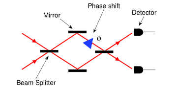
Figure 1: (Color online) Schematic of a Mach-Zehnder interferometer, with relative phase shift $\phi$ resulting from propagation of an input field through its arms.

We consider a Mach-Zehnder interferometer with two input ports $A$ and $B$, see Fig. 1, characterized by bosonic annihilation and creation operators $\hat{a}$ and $\hat{a}^{\dagger}$ and $\hat{b}$ and $\hat{b}^{\dagger}$, respectively. We restrict our investigation to a system with fixed particle number $N$, in which case its properties are conveniently described in terms of the angular momentum operators Sanders and Milburn (1995)

$$\hat{J}_{x} = \frac{\hat{a}^{\dagger}\hat{b}+\hat{b}^{\dagger}\hat{a}}{2},$$ (1)

$$\hat{J}_{y} = \frac{\hat{a}^{\dagger}\hat{b}-\hat{b}^{\dagger}\hat{a}}{2i},$$ (2)

$$\hat{J}_{z} = \frac{\hat{a}^{\dagger}\hat{a}-\hat{b}^{\dagger}\hat{b}}{2},$$ (3)

$$\hat{J}^{2} = \hat{J}_{x}^{2}+\hat{J}_{y}^{2}+\hat{J}_{z}^{2},$$ (4)

which obey the familiar commutation relations $\left[\hat{J}_{i},\hat{J}_{j}\right]=\varepsilon_{ijk}i\hat{J}_{k}$, where $\varepsilon_{ijk}$ is the Levi-Civita symbol, and $\left[\hat{J}^{2},\hat{J}_{i}\right]=0$. Choosing $z$ as the quantization axis we work in the basis of eigenstates common to $\hat{J}^{2}$ and $\hat{J}_{z}$,

$$|j,m\rangle_{z}\equiv|n_{a}\rangle|n_{b}\rangle.$$ (5)

Here $|n_{i}\rangle$ is a Fock state with $n_{i}$ particles in arm $I=A,B$. For brevity we drop the subscript $z$ henceforth. The eigenvalues corresponding to $\hat{J}^{2}$ and $\hat{J}_{z}$ are $j(j+1)$ and $m$ respectively, where

$$j=(n_{a}+n_{b})/2=N/2$$ (6)

and

$$m=(n_{a}-n_{b})/2.$$ (7)

In terms of these operators, the propagation of the input fields through the interferometer – which consists of three unitary transformations describing an input $50/50$ beam-splitter, the relative phase shift $\phi$, and an output $50/50$ beam splitter – reads Sanders and Milburn (1995)

$$|\psi_{\rm out}\rangle = e^{-i(\pi/2)\hat{J}_{x}}e^{i\phi\hat{J}_{z}}e^{i(\pi/2)\hat{J}_{x}}|\psi_{\rm in}\rangle$$ (8)

$$= e^{-i\phi\hat{J}_{y}}|\psi_{\rm in}\rangle.$$ (9)

Our aim is to find input states

$$|\psi_{\rm in}\rangle=\sum_{m=-N/2}^{N/2}\alpha_{m}|j,m\rangle$$ (10)

such that the uncertainty in the estimate of the phase $\phi$ is minimized.

Our restriction in this paper to fixed total particle number leads to considerable analytical and computational simplification, but the more general problem in which the average particle number is conserved is also of interest, and can in principle be carried out with the same techniques.

III Likelihood Function

A number of approaches have been used as measures of the uncertainty in estimate of the relative phase $\phi$. Commonly the standard error propagation formula is used to express this phase uncertainty in terms of the mean square error of a measured observable such as the particle number difference Search and Meystre (2003)

$$\Delta\phi=\Delta\hat{J}_{z}/(d\hat{J}_{z}/d\phi).$$ (11)

Probability operator measures are also used Berry et al. (2001), as well as information theoretical measures such as the Shannon mutual information Bahder and Lopata (2006). In this paper we estimate the relative phase following an operational approach based on Bayes’ theorem Braunstein (1992a); Holland and Burnett (1993); Hradil (1995); Hradil et al. (1996). Consider an experiment in which the probability amplitude of the $i^{\rm th}$ basis state of an $N+1$ dimensional Hilbert space depends on some phase $\phi$,

$$|\psi\rangle=\sum_{i=0}^{N}\alpha_{i}(\phi)|i\rangle.$$ (12)

The probability to measure $|i\rangle$ conditioned on that phase is $P(i|\phi)=|\alpha_{i}(\phi)|^{2}$, with

$$\sum_{i=0}^{N}P(i|\phi)=1.$$ (13)

Bayes’ theorem states that the probability that the phase shift has the value $\phi$, conditioned on the outcome $i$, is

$$P(\phi|i)=\frac{P(\phi)P(i|\phi)}{P(i)},$$ (14)

where $P(\phi)$ is the phase probability distribution prior to the measurement and $P(i)$ is the prior detection probability for the outcome $i$. Following a measurement with outcome $i_{1}$, the phase probability distribution becomes $P(\phi|i_{1})$, which may now be used as the prior phase probability distribution for a second measurement Holland and Burnett (1993), so that

$$P(\phi|i_{1},i_{2})=\frac{P(\phi|i_{1})P(i_{2}|\phi)}{P(i_{2})}=\frac{P(\phi)P(i_{1}|\phi)P(i_{2}|\phi)}{P(i_{1})P(i_{2})}.$$ (15)

Likewise, the phase probability distribution conditioned on the outcome of a sequence of $M$ measurements is

$$P(\phi|i_{1},i_{2},...,i_{M})=\frac{P(\phi)P(i_{1}|\phi)P(i_{2}|\phi)...P(i_{M}|\phi)}{P(i_{1})P(i_{2})...P(i_{M})}.$$ (16)

For a large number of measurements, $M\gg 1$, and assuming that the true phase shift is $\phi=\theta$, the number of times a factor $P(i|\phi)$ appears in the product (16) is approximately $P(i|\theta)M$. This motivates the introduction of a likelihood function for the phase shift to be $\phi$, conditioned on its true value being $\theta$, as Hradil (1995); Hradil et al. (1996)

$$P_{M}(\phi|\theta)=\frac{1}{\cal{N}}\prod_{i=0}^{N}P(i|\phi)^{P(i|\theta)M},$$ (17)

where

$$\mathcal{N}=\int_{-\frac{\pi}{2}}^{\frac{\pi}{2}}d\phi^{\prime}\prod_{i=0}^{N}P(i|\phi^{\prime})^{P(i|\theta)M}$$ (18)

is a normalization constant. The likelihood function $P_{M}(\phi|\theta)$ has the desirable property that it possesses a maximum at the true value, $\theta$, of the phase shift. This is easily shown by taking its derivative

$$\frac{dP_{M}(\phi|\theta)}{d\phi} = \sum\limits_{i=0}^{N}\left[MP(i|\theta)P(i|\phi)^{\left[MP(i|\theta)-1\right]}\frac{dP(i|\phi)}{d\phi}\prod_{k\neq i}^{N}P(k|\phi)^{MP(k|\theta)}\right]$$ (19)

$$= M\left[\prod_{k=0}^{N}P(k|\phi)^{MP(k|\theta)}\right]\sum\limits_{i=0}^{N}\frac{P(i|\theta)}{P(i|\phi)}\frac{dP(i|\phi)}{d\phi}.$$

Evaluating Eq. (19) at $\theta$, together with the normalization condition (13) gives then

$$\frac{dP(\phi|\theta)}{d\phi}\left.\vphantom{\frac{}{}}\right|_{\theta}=M\left[\prod_{k=0}^{N}P(k|\theta)^{MP(k|\theta)}\right]\sum\limits_{i=0}^{N}\frac{dP(i|\phi)}{d\phi}\left.\vphantom{\frac{}{}}\right|_{\theta}=0,$$ (20)

implying an extremum at $\theta$. Taking the second derivative and again using normalization shows this extremum to be a maximum.

In order to estimate the phase uncertainty in the limit of large $M$ we introduce the function

$$K(\phi|\theta)=\log{P(\phi|\theta)}.$$ (21)

Expanding then $K(\phi|\theta)$ around $\phi=\theta$ and accounting for the normalization condition (13) we find that $P(\phi|\theta)$ is approximately given by

$$P(\phi|\theta)\approx e^{K(\theta|\theta)-\frac{(\phi-\theta)^{2}}{2\sigma^{2}}}$$ (22)

where

$$\sigma^{2}=\frac{1}{M\sum_{i=0}^{N}\left(\frac{dP(i|\phi)}{d\phi}|_{\theta}\right)^{2}/P(i|\theta)}=\frac{1}{MF},$$ (23)

and

$$F=\sum_{i=0}^{N}\left(\frac{dP(i|\phi)}{d\phi}\Big{|}_{\theta}\right)^{2}/P(i|\theta)$$ (24)

is the so-called Fisher information, as shown in Appendix A Cover and Thomas (2006). For large $M$ the exponential suppresses strongly those contributions to $P(\phi|\theta)$ for which $\phi\gtrsim\sigma$ so that $P(\phi|\theta)$ becomes Gaussian in that limit Braunstein (1992a). Asymptotically, the likelihood function is therefore completely characterized by its variance, or equivalently by its Fisher information. Equation (23) also shows that the phase uncertainty decreases as the inverse square root of the number of measurements.

The Fisher information plays an important role in information theory as it gives a lower limit to the variance of any estimator via the Cramer-Rao inequality Cover and Thomas (2006)

$${\rm var}(x)\geq\frac{1}{F},$$ (25)

where ${\rm var}(x)$ is the mean square error of the random variable $x$ being estimated and Eq. (25) is the defining relation for the Fisher information. (Note also that the Fisher information of $M^{\prime}$ independent and identically distributed samples is $M^{\prime}$ times the individual Fisher information.) Thus Eq. (22) indicates that the likelihood function $P_{M}(\phi|\theta)$ achieves the Cramer-Rao limit. It permits us to find input states of the interferometer of the form of Eq. (10) that result in an estimate of the phase shift with minimum uncertainty.

To illustrate how the likelihood function may be used to estimate a phase shift experimentally, consider a thought experiment using the Mach-Zehnder interferometer in Fig. 1. Each measurement counts the number of particles $n_{a}$ exiting the interferometer in arm “A”. Due to particle conservation, this is a direct measure of the quantum number $m$. Expanding the exit state of the field as

$$|\psi_{\rm out}(\phi)\rangle=\sum_{m}\alpha_{m}(\phi)|j,m\rangle,$$ (26)

each measurement yields a specific particle number $n^{(i)}_{a}=N/2+m^{(i)}$ with an associated phase probability distribution

$$P(m^{(i)}|\phi)=|\alpha_{m}^{(i)}(\phi)|^{2}.$$ (27)

After $M$ such measurements the conditional phase probability distribution takes the form of Eq. (16), which for sufficiently large $M$ is a good approximation to the likelihood function Eq. (17) — up to the normalization constant as in Eq. (18). The maximum of this conditional phase probability distribution is an estimate of the phase shift and its variance gives the uncertainty.

An important consideration is the number of measurements needed for the conditional phase probability distribution, Eq. (16), to be an accurate representation of the likelihood function. This matter is not addressed in this paper where we use throughout the assymptotic form of the likelihood function, but has been investigated by Braunstein Braunstein (1992b).

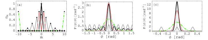
Figure 2: (Color online) (a) Probability amplitudes $\alpha_{m}$ for the twin-Fock state (solid black line), the external N00N state (green dot-dashed line), the internal N00N state Eq. (31) (solid gray line) and the di-Fock state $|\psi_{\rm di}(q=1)\rangle$ (red dotted line). Corresponding likelihood functions for (b) ($M=1)$ and (c) ($M=10)$. In the di-Fock state secondary peaks are already almost completely absent for $M=1$, thus concentrating more probability density around $\phi=0$. Secondary features are however suppressed for larger values of $M$ in all cases, indicating that the twin-Fock state results in a slightly smaller phase uncertainty.

IV Results

This section summarizes results of a numerical search for optimum input states of the interferometer. This search employed the global optimization protocol of simulated annealing Bohachevsky et al. (1986); Press et al. (1999), whose main features are summarized in Appendix B.

To set the stage for this discussion, we first recall that several states have previously been proposed as good candidates for Heisenberg limited interferometry. One such state is the balanced twin-Fock input state Kim et al. (1998); Pezzé and Smerzi (2006)

$$|\psi_{\rm tw}\rangle=|j,0\rangle\equiv|N/2\rangle_{a}|N/2\rangle_{b},$$ (28)

a state that we use as a benchmark in the following discussion. It was suggested in Refs. Yurke (1986); Pezzé and Smerzi (2006) that improvements over that state can be achieved by using instead the state

$$|\psi_{\rm di}(q)\rangle=1/\sqrt{2}\left(|j,q\rangle+|j,-q\rangle\right),$$ (29)

with $q=1$. This state, which we refer to as a di-Fock state in the following, presents the advantage of suppressing secondary peaks in the likelihood function, thus concentrating more probability density around the true value of the phase shift.

It has also been proposed that Heisenberg limited phase sensitivity can be achieved with the so-called N00N state Bollinger et al. (1996)

$$|\psi_{\rm N00N}\rangle\equiv|\psi_{\rm di}(q=j)\rangle = 1/\sqrt{2}\left(|j,j\rangle+|j,-j\rangle\right)$$

$$= 1/\sqrt{2}\left(|N\rangle_{a}|0\rangle_{b}+|0\rangle_{a}|N\rangle_{b}\right).$$

Some disagreement exists in the current literature regarding the phase sensitivity of N00N states, with some authors claiming that it in fact obeys shot noise limited sensitivity Pezzé and Smerzi (2006). Mitchell et al. Mitchell et al. (2004) as well as Walther et al. Walther et al. (2004) have pointed out that $N00N$ states may be used to produce super-resolving phase oscillations, with a period of $2\pi/N$, in interferometric measurements. In agreement with this we will show that similar oscillations occur in the likelihood function, if Eq. (30) describes the state of the system after the first beam splitter. To be explicit we distinguish between external N00N states for which Eq. (LABEL:noon) is the state before the first beam splitter, and internal N00N states for which Eq. (LABEL:noon) is the state after the first beam splitter. The internal N00N state is equivalent to using an input state

$$e^{-i\hat{J}_{x}\pi/2}|\psi_{\rm N00N}\rangle.$$ (31)

It can also be achieved by using as an input the state $|N\rangle_{a}|0\rangle_{b}$ and replacing the first beam splitter with a non-linear beamsplitter with appropriate interaction time, as shown in Mølmer and Sørensen (1999).

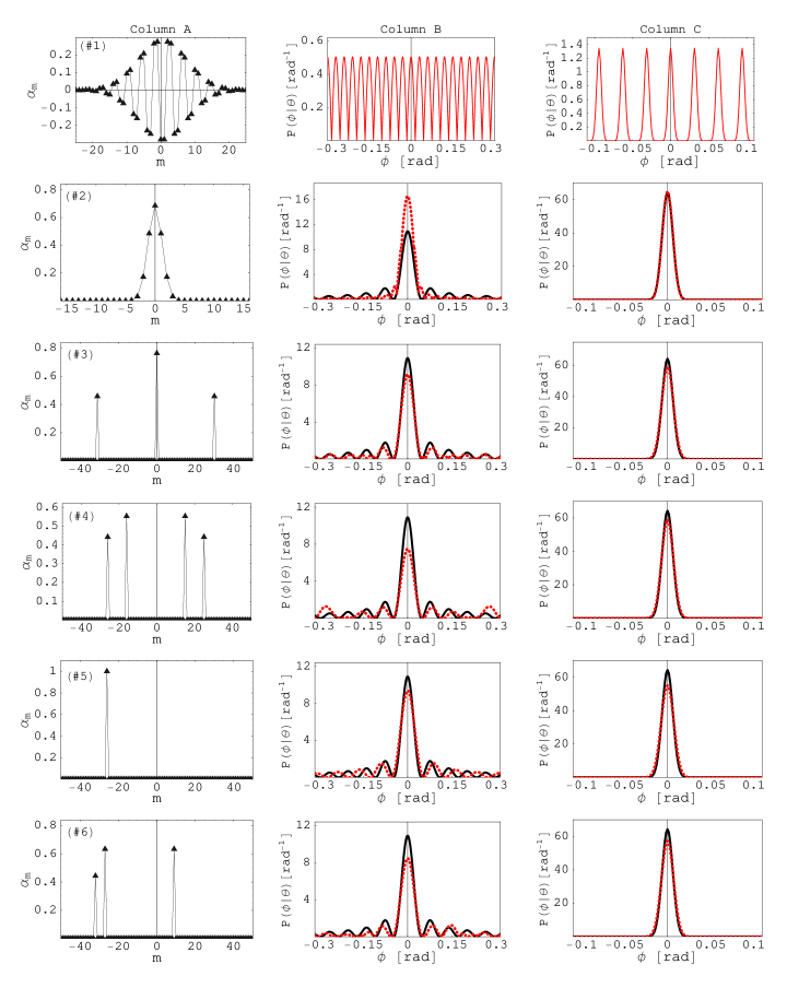
Figure 3: (Color online) Column A: probability amplitudes for several possible input states with $N=100$ particles. Column B: Corresponding likelihood functions for $M=1$ (dotted red line), compared to the result for the benchmark twin-Fock input (solid black line). Column C: Likelihood functions for ($M=10$).

Figure 2(a) shows the probability amplitudes $\alpha_{m}$ of the basis states $|j,m\rangle$ for the input states of Eqs. (28)-(29), as well as the external N00N and internal N00N states, for a system with $N=20$ particles, and a relative phase $\theta=0$ between the two arms of the interferometer. The solid black line corresponds to the twin-Fock input, the dotted red line to the input state $|\psi_{\rm di}(q=1)\rangle$, the green dot-dashed line to the external N00N state and the gray solid line to the internal N00N state . The corresponding likelihood functions for $M=1$ are plotted in Fig. 2 (b). Apart from the internal N00N state the probability density is concentrated close to $\phi=0$ in all cases, but the di-Fock state seems more favorable as it results in a narrow distribution with no significant secondary peaks. However, this apparent advantage rapidly disappears for larger $M$, in which case the secondary peaks associated with the twin-Fock state are suppressed, leading to a slightly narrower distribution. Note the distribution corresponding to the external N00N state remains considerably wider than the other candidates, indicating a larger uncertainty in the phase estimate. The likelihood function of the internal N00N state rapidly oscillates with a period of $2\pi/N$ radians. This is consistent with the $N$-fold increase in phase oscillations observed in Walther et al. (2004); Mitchell et al. (2004).

Figure 3 illustrates some of the large number of possible input states numerically obtained from the simulated annealing algorithm for a system of $N=100$ particles. Column A plots the probability amplitudes $\alpha_{m}$ of the input states; column B shows the corresponding likelihood functions with $M=1$ (broken red broken lines) and compares them to the likelihood function of the benchmark twin-Fock input (solid black lines); column C plots the situation for $M=10$ measurements. A remarkable feature of these results is that while these input states are very markedly different, their likelihood functions become almost indistinguishable for large $M$. Surprisingly perhaps the optimization procedure clearly shows the existence of a large number of local minima resulting in almost identical likelihood functions.

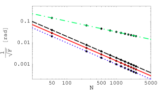
Figure 4: (Color online) Scaling of the inverse square root Fisher information, $\sigma=1/\sqrt{F}$ with particle number for the state in row 1 of Fig. 3 (blue dotted line), twin-Fock state (solid red line), the “gaussian state” (black dashed line) and the external N00N state (green dot-dashed line). The points are calculated using Eq. (24) while the lines correspond to least square fits, with the values external N00N state: $\sigma=1.0/N^{1/2}$, “gaussian”: $\sigma=1.9/N$, twin-Fock: $\sigma=1.4/N$ and state in row 1 of Fig. 3: $\sigma=1.0/N$. Note the log-log scale.

To demonstrate that all states identified by the simulated annealing algorithm indeed result in approximate Heisenberg limited phase sensitivity, Fig. 4 shows a log-log plot of the inverse square root Fisher information, $1/\sqrt{F}$, as a function of particle number over a range of $50\leq N\leq 2500$. The solid red line is for twin-Fock states, the green dot-dashed line for external N00N states, the dotted blue line for the uppermost state in Fig. 3, and the dashed black line for the state in row 2 of Fig. 3. For clarity we refer to the latter state as a ”gaussian state” in the following. All lines are least square fits of the equation

$$\sigma=\frac{C}{N^{\beta}},$$ (32)

where $C$ and $\beta$ are fit parameters.

Table 1 summarizes the results of this fit for the states of Fig. 3, the number referring to the row number in the figure. Up to differences of a few percent in the overall proportionality constant $C$, all of these states clearly satisfy the $1/N$ scaling characteristic of Heisenberg limited sensitivity, the only notable exception being the external N00N state, which (in agreement with Pezzé and Smerzi Pezzé and Smerzi (2006)) is shot-noise limited. On the other hand, the inverse square root Fisher information of the internal $N00N$ state does scale with the Heisenberg limit. Despite this, the rapid oscillations in the likelihood function seen in Fig. 2(b) and (c) allow a phase estimate only modulo $2\pi/N$. The consequent ambiguities imply that the internal N00N state may not be useful for phase estimation when using the current Bayesian analysis unless one has a priori knowledge that the phase shift lies within a particular phase-bin of width $2\pi/N$. We now discuss the candidates obtained by search algorithms in turn.

The state with the highest Fisher information that we found, an apparent global optimum, is shown in row 1 of Fig. 3. The envelope of its probability amplitudes $\alpha_{i}$ is a Gaussian with width $w=\sqrt{N}$. Despite the high Fisher information of that state, though, it produces a significant ambiguity in the determination of the phase estimate as secondary peaks persist even for $M=10$, as seen in column C. A feature not apparent on the scale in this figure is that the central peak is the absolute maximum and becomes increasingly dominant for increased $M$. Yet, as in the case of the internal N00N state, the persistence of secondary peaks for relatively large sequences of measurements indicates that it may not be the most useful state in practice.

In the case of the “gaussian state”, second row of Fig. 3, the probability amplitudes $\alpha_{m}$ have a Gaussian distribution around the state $|j,m=0\rangle$,

$$\alpha_{m}=\exp{\left[-m^{2}/\sigma^{\prime 2}\right]}/\cal{N^{\prime}},$$

where $\cal{N}^{\prime}$ is a normalization constant, and the standard deviation is $\sigma^{\prime}=1.7$ for the example at hand. That state results in Heisenberg limited sensitivity for $0<\sigma^{\prime}\lesssim j$, with

$$\frac{1}{\sqrt{F}}\approx\frac{\sigma^{\prime}}{N}.$$ (33)

The limit $\sigma^{\prime}\rightarrow 0$ corresponding to the twin-Fock state.

State	$1/\sqrt{F}=C/N^{\beta}$
$|j,0\rangle$	$1.4/N$
External N00N state	$1.0/N^{1/2}$
Internal N00N state	$1.0/N$
$|\psi_{di}(q=1)\rangle$	$2.0/N$
#1	$1.0/N$
#2	$1.9/N$
#3	$1.5/N$
#4	$1.5/N$
#5	$1.7/N$
#6	$1.6/N$

Table 1: Scaling of the phase uncertainty as a function of the particle number $N$ for the the twin state, the external- and internal N00N states, the di-Fock state, and the input states of Fig. 3.

The state described in the third row of Fig. 3 is an example of a state we refer to as a tri-Fock state, and it has the form

$$|\psi_{\rm tri}(q)\rangle=\left(\alpha_{-}|j,-q\rangle+\alpha_{0}|j,0\rangle+\alpha_{+}|j,q\rangle\right)/\cal{N}^{\prime},$$ (34)

where $\cal{N}^{\prime}$ is a normalization constant. We find numerically that it results in Heisenberg limited sensitivity for any value of $q$.

The fourth row in Fig. 3 describes a state that is a superposition of four Fock states. For the $N=100$ particles considered in our simulations, and the state in row one of Fig. 3 aside, we have found states with superpositions containing up to $\sim 8$ Fock states that result in Heisenberg- limited sensitivity.

We also found that di-Fock states, Eq. (29), with arbitrary $q$ generally result in Heisenberg limited or near Heisenberg limited scaling for $q$ as large as $q\lesssim 0.98j$. For larger $q$ the state approaches the shot-noise limited external N00N state.

Several general trends can be noted in the results of our search. First, we find that the scaling of Eq. (32) depends only weakly on the relative probability amplitudes $\alpha_{M}$ of the Fock states involved. Changing the relative amplitudes of these coefficients by factors as large as 3 typically results in changes in the coefficient $C$ by a few percent only. The Gaussian state is a notable exception to this trend, and obeys instead the scaling equation (33).

Second, we found no inherent symmetry in the input states that result in the Heisenberg limit. This is illustrated by the states of rows 5-6 in Fig. 3. For example, the state of row 5 is an unbalanced twin-Fock state of the form

$$|\psi_{\rm tw}\rangle=|j,\gamma j\rangle,$$ (35)

where $\gamma$ is some fraction. We found numerically that the state resulted in Heisenberg limited sensitivity for $0.02\lesssim\gamma\lesssim 0.98$.

All states shown in Fig. 3 have real amplitudes. Allowing for complex amplitudes of the same magnitudes retains Heisenberg limited or near Heisenberg limited scaling, with $\beta\gtrsim 0.95$ in Eq. (32) and the coefficient $C$ changed by only a few percent. Again the effect is more pronounced in the Gaussian state, where the change in $C$ can be up to a factor of $\sim 2$. This is because that state has neighboring states occupied, and the number statistics of these states influence each other even for small phase shifts.

Due to the existence of numerous input states resulting in nearly identical uncertainties within the measurement scheme presented here, a more relevant criterion for the selection of an appropriate input state is likely to be its ease of experimental realization. We address this point in some more detail in the next section for the case of the ”gaussian state.”

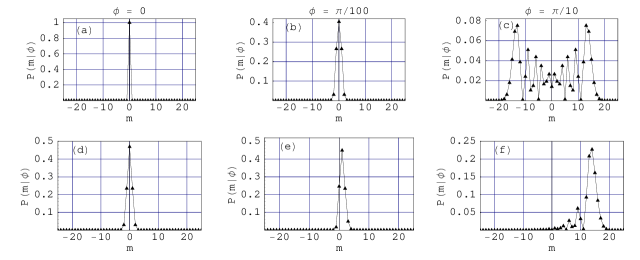
Figure 5: (Color online) Number statistics for phase shifts of $\phi=0$, $\phi=\pi/100$ and $\phi=\pi/10$ in a system with $N=100$ particles for (a)-(c) a twin-Fock input state and (d)-(f) a ”gaussian” input state. The twin-Fock state populates number states symmetrically around $m=0$, leading to an expectation value of $\langle\hat{J}_{z}\rangle=0$ for all values of $\phi$. This is not the case for a gaussian state.

V The Gaussian state

The “gaussian” input state is a promising candidate for Heisenberg limited interferometry for two reasons: (1) there is a simple experimental scheme available to generate it; (2) as we show below, the expectation value of $\hat{J}_{z}$ is phase dependent in that case (as opposed to the situation for twin-Fock input states) providing an alternative phase estimate to the direct measurement of the likelihood function, while still allowing Heisenberg limited sensitivity.

V.1 Number statistics

As mentioned in section III, the likelihood function can be experimentally reconstructed by multiplying the phase probability distributions $P(i|\phi)$ associated with a sequence of measurement outcomes. This is the approach that was adopted in the simulations carried out in Refs. Holland and Burnett (1993); Kim et al. (1998) for twin-Fock input states. In that case however the average particle number difference remains zero for all relative phase shifts between the interferometer arms, and is therefore not a useful observable. The same is true for the majority of the states that we identified in our numerical optimization search. One way to circumvent this difficulty is to measure instead the variance of $\hat{J}_{z}$, an approach that still results in Heisenberg limited estimates. However, as was pointed out in Ref. Kim et al. (1998) for the case of the twin-Fock state, the signal to noise ratio is then small, $\langle\hat{J}_{z}^{2}\rangle/\sqrt{\langle\hat{J}_{z}^{4}\rangle-\langle\hat{J}_{z}^{2}\rangle^{2}}=\sqrt{2}$.

One advantage of using a gaussian input state instead is that $\langle\hat{J}_{z}\rangle$ now depends on the relative phase $\phi$. This is illustrated in Fig. 5(a)-(c), which shows the probability distribution $P(m|\phi)$ at the exit of the interferometer for twin-Fock and gaussian input states, and for phase shifts $\phi=0$, $\phi=\pi/100$ and $\phi=\pi/10$. The expectation value of $\hat{J}_{z}$ for the Gaussian state is clearly not equal to zero for non-zero phase shifts, and may therefore be used directly to estimate that shift. The uncertainty in $\hat{J}_{z}$, evaluated via the standard error propagation formula Eq. (11), is shown in Fig. 6 as a function of the number of interfering particles. Least square fits indicate that the uncertainties are Heisenberg limited, with $\Delta\phi=2.0/N$ for the gaussian state and similarly $\Delta\phi=2.4/N$ in the case of a tri-Fock state with $q=1$.

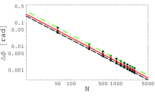
Figure 6: (Color online) Scaling of the uncertainty in the estimate of the relative phase from a measurement of average particle number difference. The dashed black line is for a Gaussian state and the red solid line of a tri-Fock state, Eq. (34), with $q=1$, and the green dot-dashed line represents the state engineered as described in section V(B). The points are numerically determined while the lines correspond to least square fits. Note the log-log scale.

V.2 Input state engineering

We have seen that the constraints on the relative phases of the complex probability amplitudes $\alpha_{i}$ of the input states are surprisingly weak when estimating phase shifts $\phi$ via a reconstruction of the likelihood function. However, the number statistics of the field after passage through the interferometer depend critically on these relative phases. For example, if in the Gaussian state of Fig. 3 the components $|j,-1\rangle$ and $|j,+1\rangle$ are $\pi/2$ radians out of phase with $|j,0\rangle$, the output state $|\psi_{\rm out}\rangle$ will be populated symmetrically around $|j,0\rangle$ independently of $\phi$, so that $\langle\hat{J}_{z}\rangle=0$ for all $\phi$. Hence, some care must be taken in preparing the input states $|\psi_{\rm in}\rangle$.

It is possible to generate a gaussian input state from an initial twin-Fock state, Eq. (28), by subjecting it to the Hamiltonian

$$H_{x}=\hbar g\hat{J}_{x},$$ (36)

where $g$ is a coupling constant, for a time $\tau=3\pi/4Ng$. The resulting state is precisely the state shown in row 2 of Fig. 3, but with the probability amplitudes of the components $|j,-1\rangle$ and $|j,+1\rangle$ $\pi/2$ radians out of phase with the component $|j,0\rangle$. These three components can be brought into phase via an additional evolution under the Hamiltonian

$$H_{z}=\hbar\chi\hat{J}_{z}^{2}$$ (37)

for a time $\tau=3\pi/2\chi$. The resulting state allows Heisenberg limited phase estimation by measuring $\langle\hat{J}_{z}\rangle$, with the scaling law $\Delta\phi=3.2/N$ as a function of the particle number $N$. We remark that while the time evolution (37) of the input state brings the three main components of $|\psi_{\rm in}\rangle$ in phase with each other, that is not so for the other, weakly populated number states that comprise it. This results in a somewhat reduced performance compared to Gaussian state with all components in phase.

Hamiltonians of the form Eq. (37) have long been known to act as squeezing operators in interferometers Kitagawa and Ueda (1993). In the case of photons, they can be implemented by inserting an optical Kerr medium into each arm of the interferometer Kitagawa and Yamamoto (1986). In the case of charged particles they arise due to mutual phase modulation from Coulomb interaction between particles in each arm Kitagawa and Ueda (1991). Atomic spins coupled to the polarization of an optical field Smith et al. (2006); Geremia et al. (2006) can lead to similar Hamiltonians for neutral atoms.

VI Conclusion

We have used a global optimization scheme to systematically search for input states of a quantum mechanical Mach-Zehnder interferometer that yield phase estimates with accuracy scaling like the inverse number of particles, the Heisenberg limit. Surprisingly perhaps, we find that a large number of states can achieve that limit. They typically consist of superpositions of a small number of Fock states, with few restrictions on the relative phase of their complex amplitudes on on their symmetry. An input state of particular relevance consists of a gaussian distribution of amplitudes around the state $|N/2\rangle_{a}|N/2\rangle_{b}$, due principally to its relative ease of realization with simple Hamiltonian dynamics.

Appendix A Fisher information

Consider the deviation $\langle\delta A_{\theta}\rangle$ of an observable from its mean value $\langle A(\theta)\rangle$ at a fixed phase $\theta$, as a function of the phase shift $\phi$,

$$\langle\delta A_{\theta}\rangle=\sum\limits_{j}\left(a_{j}-\langle A(\theta)\rangle\right)P(j|\phi).$$ (38)

Then

$$\frac{d\langle\delta A_{\theta}\rangle}{d\phi} = \sum\limits_{j}\left(a_{j}-\langle A(\theta)\rangle\right)\frac{dP(j|\phi)}{d\phi}$$ (39)

$$= \sum\limits_{j}\left(a_{j}-\langle A(\theta)\rangle\right)P(j|\phi)\frac{\log{P(j|\phi)}}{d\phi}.$$ (40)

Regrouping the factors in Eq. (40) and squaring gives

$$\left[\frac{d\langle\delta A_{\theta}\rangle}{d\phi}\right]^{2} = \left[\sum\limits_{j}\left(\left(a_{j}-\langle A(\theta)\rangle\right)\sqrt{P(j|\phi)}\right)\left(\sqrt{P(j|\phi)}\frac{\log{P(j|\phi)}}{d\phi}\right)\right]^{2}$$ (41)

$$\leq \left[\sum\limits_{j}P(j|\phi)\left(\frac{\log{P(j|\phi)}}{d\phi}\right)^{2}\right]\left[\sum\limits_{j}\left(a_{j}-\langle A(\theta)\rangle\right)^{2}P(j|\phi)\right],$$ (42)

where we have used the Schwarz inequality in the last step. Noting that the second term in Eq. (39) vanishes due to normalization we have $d\langle\delta A_{\theta}\rangle/d\phi=d\langle A\rangle/d\phi$. We can then rewrite inequality (42) and evaluate it at $\theta$ to give the desired result:

$$\Delta\phi^{2}=\frac{\Delta A^{2}}{\left[d\langle A\rangle/d\phi\right]^{2}}\geq\frac{1}{\sum\limits_{j}P(j|\theta)\left(\frac{\log{P(j|\phi)}}{d\phi}\arrowvert_{\theta}\right)^{2}}.$$ (43)

This is the Cramer-Roa inequality, Eq. (25), in the current context. The denominator on the right in Eq. (43) defines the Fisher information.

Appendix B Simulated annealing

Simulated annealing Bohachevsky et al. (1986); Press et al. (1999) is a mathematical approach to global optimization simulating the metallurgical process whereby an amorphous compound is successively heated and cooled while gradually lowering the average temperature in an attempt to enlarge the grain size of single crystals in the compound. The protocol is as follows:
1. Initial conditions for the optimization parameters, $\mathbf{x}=(x_{1},x_{2},...x_{r})$ are chosen, usually at random.
2. With each allowed value of $\mathbf{x}$ is associated an pseudo-energy, $E(\mathbf{x})$, which is the quantity to be minimized.
3. A new value, $\mathbf{x}^{\prime}=\mathbf{x}+\mathbf{\Delta x}$, is then generated for the optimization parameters, and the change in energy $\Delta E=E(\mathbf{x}^{\prime})-E(\mathbf{x})$ calculated.
4. The new value of $\mathbf{x}$ always replaces the old if $p=e^{-\Delta E/kT}>1$, or with probability $p$ if $p<1$. Here $k$ is a constant of proportionality analogous to Boltzmann’s constant in statistical mechanics, and $T$ is a pseudo-temperature.
5. The process is repeated.

Accepting new parameter sets for which $p<1$, i.e. uphill steps on the energy manifold, allows the algorithm to explore the whole parameter space instead of converging directly to the closest local minimum.

Two important considerations in this procedure are the method of choosing the next set of parameters $\mathbf{x}^{\prime}$ and the annealing schedule, i.e. the protocol for gradually lowering the temperature with intermittent heating cycles until the system has frozen into, hopefully, a global minimum. Various approaches to these considerations have been discussed in the literature Vanderbilt and Louie (1984); Bohachevsky et al. (1986).

In our implementation the optimization parameters are the set of amplitudes $\alpha_{m}$ of the input state vector Eq. (10) and the energy the inverse square root of the Fisher information. We execute the simulated annealing algorithm not on a single vector $\mathbf{\bar{\alpha}}$, but a population of vectors chosen at random. The pseudo-temperature of the system is set by the average energy of the population,

$$T=\frac{1}{P}\sum\limits_{i=1}^{P}1/\sqrt{F_{i}},$$ (44)

where $P$ is the number of state vectors in the population and $F_{i}$ the Fisher information of the $i^{\rm th}$ state vector. Defining the temperature in this way self-regulates the cooling cycle. If a single global minimum exists, the algorithm will continue sampling until the majority of state vectors have fallen into the global minimum. On the other hand if many local minima of comparable depth exist the algorithm will also continue to sample the parameter space until the majority of state vectors have found such local minima. As more local minima are found the system ”cools down” by itself.

When the state vectors $\bar{\alpha}$ have converged near the minima and the step size $|\Delta\bar{\alpha}|=|\bar{\alpha}^{\prime}-\bar{\alpha}|$ is fixed, all new steps $\bar{\alpha}^{\prime}$ will be uphill, thus halting further convergence. To enable further convergence we therefore half the step size when the number of downhill steps found over a several iterations drops below a threshold.

It may also happen in our approach that the system reaches an equilibrium condition in which the average number of uphill steps accepted become equal to the average number of downhill steps found. To ensure that the system continues to converge towards minima, we lower Boltzmann’s constant by $k\rightarrow 0.9k$ if this point is reached. We take as an indicator that the system is near this point whenever the number of accepted uphill steps is larger than the number of downhill steps in a given iteration cycle.

To summarize the algorithm:

1. Choose initial population at random and calculate pseudo-temperature

2. Find new state vectors $\bar{\alpha}^{\prime}=\bar{\alpha}+\Delta\bar{\alpha}$ and replaces the old if $p=e^{-\Delta E/kT}>1$, or with probability $p$ if $p<1$

3. If the number of uphill steps accepted is greater than number of downhill steps decrease $k\rightarrow 0.9k$.

4. If the number of downhill steps found is less than specified threshold reduce $\Delta\bar{\alpha}\rightarrow 0.5\Delta\bar{\alpha}$.

5. Repeat algorithm

We have implemented searches that assume either real or complex amplitudes. In addition, in some searches we imposed no restrictions on the symmetry of input states, while in others we forced the input states to be either symmetric or anti-symmetric around $|N/2\rangle_{a}|N/2\rangle_{b}$.

In the case of real amplitudes, the initial population was chosen by generating a random number between $[-1,1]$ for each $\alpha_{m}$ and then normalizing the state vector. For complex amplitudes the magnitudes $|\alpha_{m}|$ were chosen at random between 0 and 1 and a complex phase between 0 and 2$\pi$.

We have used two different approaches to specifying the new state vectors $\bar{\alpha}^{\prime}$ during each iteration. In the first one new state vectors were selected by changing each amplitude at random within an interval $\epsilon\alpha_{m}<\alpha^{\prime}_{m}<(1+\epsilon)\alpha_{m}$, with $\epsilon<1$ and then renormalizing the state vector. In the case of complex amplitudes a new phase was also chosen as $\phi_{m}^{\prime}=\phi_{m}+\Delta\phi$ where $-\varepsilon<\Delta\phi<\varepsilon$, while in the case of real amplitudes sign changes were allowed if $|\alpha_{m}|<0.02$ by choosing $-(1+\epsilon)|\alpha_{m}|<\alpha^{\prime}_{m}<(1+\epsilon)|\alpha_{m}|$. In this approach, step (4) in the algorithm described above was rather insensitive to the values chosen for $\epsilon$ and $\varepsilon$. They were therefore taken to have fixed values $\epsilon=0.5$ and $\varepsilon=0.05$.

In the second approach each vector $\mathbf{\bar{\alpha}}$ is specified by a set of angles such that the vector moves on a hyperspherical surface of radius $1$ to ensure normalization. The next vector is chosen in a random direction on the hyper-sphere with the initial step size $\Delta\bar{\theta}=0.1$. It is decreased in successive iterations according to step (5) in the algorithm above.

In the first approach the state vectors in the population settle in many local minima of comparable depths, while in the second approach all state vectors converge to an apparent global minimum which is the state shown in row 1 of column A in Fig. 3.

References

- Grangier et al. (1987) P. Grangier, R. E. Slusher, B. Yurke, and A. LaPorta, Phys. Rev. Lett. 59, 2153 (1987).
- Xiao et al. (1987) M. Xiao, L. A. Wu, and H. J. Kimble, Phys. Rev. Lett. 59, 278 (1987).
- Yurke (1986) B. Yurke, Phys. Rev. Lett. 56, 1515 (1986).
- Holland and Burnett (1993) M. J. Holland and K. Burnett, Phys. Rev. Lett. 71, 1355 (1993).
- Sanders and Milburn (1995) B. C. Sanders and G. J. Milburn, Phys. Rev. Lett. 75, 2944 (1995).
- Kim et al. (1998) T. Kim, O. Pfister, M. J. Holland, J. Noh, and J. L. Hall, Phys. Rev. A 57, 4004 (1998).
- Combes and Wiseman (2005) J. Combes and H. M. Wiseman, J. Opt. B: Quantum Semiclass. Opt 7, 14 (2005).
- Pezzé and Smerzi (2006) L. Pezzé and A. Smerzi, Phys. Rev. A 73, 011801(R) (2006).
- Mølmer and Sørensen (1999) K. Mølmer and A. Sørensen, Phys. Rev. Lett. 82, 1835 (1999).
- Sackett et al. (2000) C. A. Sackett, D. Kielpinski, B. E. King, C. Langer, V. Meyer, C. J. Myatt, M. Rowe, Q. A. Turchette, W. M. Itano, D. J. Wineland, et al., Nature 404, 256 (2000).
- Leibfried et al. (2004) D. Leibfried, M. D. Barret, T. Schaetz, J. Britton, J. Chiaverini, W. M. Itano, J. D. Jost, C. Langer, and D. J. Wineland, Science 304, 1476 (2004).
- Walther et al. (2004) P. Walther, J. Pan, M. Aspelmeyer, R. Ursin, S. Gasparoni, and A. Zeilinger, Nature 429, 158 (2004).
- Mitchell et al. (2004) M. W. Mitchell, J. S. Lundeen, and A. M. Steinberg, Nature 429, 161 (2004).
- Berry et al. (2001) D. W. Berry, H. M. Wiseman, and J. K. Breslin, Phys. Rev. A. 63, 053804 (2001).
- Denot et al. (2006) D. Denot, T. Bschorr, and M. Freyberger, Phys. Rev. A. 73, 013824 (2006).
- Söderholm et al. (2003) J. Söderholm, G. Björk, B. Hessmo, and S. Inoue, Phys. Rev. A 67, 053803 (2003).
- Search and Meystre (2003) C. P. Search and P. Meystre, Phys. Rev. A. 67, 061601(R) (2003).
- Wang and Javanainen (2007) T. Wang and J. Javanainen, Phys. Rev. A 75, 013605 (2007).
- Bahder and Lopata (2006) T. B. Bahder and P. A. Lopata, Phys. Rev. A 74, 051801(R) (2006).
- Braunstein (1992a) S. L. Braunstein, Phys. Rev. Lett. 69, 3598 (1992a).
- Hradil (1995) Z. Hradil, Phys. Rev. A 51, 1870 (1995).
- Hradil et al. (1996) Z. Hradil, R. Myska, J. Perina, M. Zawisky, Y. Hasegawa, and H. Rauch, Phys. Rev. Lett. 76, 4295 (1996).
- Cover and Thomas (2006) T. M. Cover and J. A. Thomas, Elements of Information Theory (Wiley & Sons, Inc., 2006), 2nd ed.
- Braunstein (1992b) S. L. Braunstein, J. Phys. A: Math. Gen. 25, 3813 (1992b).
- Bohachevsky et al. (1986) I. O. Bohachevsky, M. E. Johnson, and M. L. Stein, Technometrics 28, 209 (1986).
- Press et al. (1999) W. H. Press, S. A. Teukolsky, W. T. Vetterling, and B. P. Flannery, Numerical recipes in C. The art of scientific computing (Cambridge University Press, 1999), 2nd ed.
- Bollinger et al. (1996) J. J. Bollinger, W. M. Itano, D. J. Wineland, and D. J. Heinzen, Phys. Rev. A 54, R4649 (1996).
- Kitagawa and Ueda (1993) M. Kitagawa and M. Ueda, Phys. Rev. A 47, 5138 (1993).
- Kitagawa and Yamamoto (1986) M. Kitagawa and Y. Yamamoto, Phys. Rev. A 34, 3974 (1986).
- Kitagawa and Ueda (1991) M. Kitagawa and M. Ueda, Phys. Rev. Lett. 67, 1852 (1991).
- Smith et al. (2006) G. A. Smith, A. Silberfarb, I. H. Deutsch, and P. S. Jessen, Phys. Rev. Lett. 97, 180403 (2006).
- Geremia et al. (2006) J. M. Geremia, J. K. Stockton, and H. Mabuchi, Physical Review A 73, 042112 (2006).
- Vanderbilt and Louie (1984) D. Vanderbilt and S. G. Louie, Journal of computational physics. 56, 259 (1984).