Quantum theory of degenerate $\chi^{(3)}$ two-photon state

Jun Chen, Kim Fook Lee, and Prem Kumar Center for Photonic Communication and Computing, EECS Department
Northwestern University, 2145 Sheridan Road, Evanston, IL 60208-3118

We develop a theory to model the degenerate two-photon state generated by the 50/50 Sagnac-loop source. We start with an interaction Hamiltonian that is capable of describing the interaction among the four optical fields (non-degenerate pump and degenerate signal/idler), which reads:

$\displaystyle H_{I}(t)$ $\displaystyle=$ $\displaystyle\alpha\int dV(E_{s}^{(-)}E_{i}^{(-)}E_{p1}^{(+)}E_{p2}^{(+)}+{\rm H.c.})$ (1)

where $\alpha$ is a material constant that is characteristic of the optical fiber being used. The non-degenerate pump field is taken to be two synchronous pulses (denoted by subscripts $p1$ and $p2$), copolarized and co-propagating down the fiber axis (denoted as z direction here), with central frequencies $\Omega_{p1}$ and $\Omega_{p2}$ and envelope shapes $\overline{E}_{p1}$ and $\overline{E}_{p2}$. Mathematically, they are written as below

$\displaystyle E_{p1}^{(+)}$ $\displaystyle=$ $\displaystyle\int d\omega_{p1}\overline{E}_{p1}(\omega_{p1})\,e^{ik(\omega_{p1})z-i\omega_{p1}t}\,e^{-i\gamma P_{1}z}\,,$ (2)
$\displaystyle E_{p2}^{(+)}$ $\displaystyle=$ $\displaystyle\int d\omega_{p2}\overline{E}_{p2}(\omega_{p2})\,e^{ik(\omega_{p2})z-i\omega_{p2}t}\,e^{-i\gamma P_{2}z}\,,$ (3)

where $\omega_{p1}=\Omega_{p1}+\nu_{p}$ and $\omega_{p2}=\Omega_{p2}+\nu^{\prime}_{p}$ are the frequency arguments for the two pump fields. $\nu_{p}$ ($\nu^{\prime}_{p}$) denotes the frequency component within $p1$’s ($p2$’s) spectrum that deviates from its central frequency $\Omega_{p1}$ ($\Omega_{p2}$) by that amount. The phase tags $e^{-i\gamma P_{1}z}$ and $e^{-i\gamma P_{2}z}$ are induced by $p1$’s and $p2$’s self-phase modulation (SPM) respectively, and are included in a straightforward manner. Note that $P_{1}$ and $P_{2}$ denote the peak powers of $p1$ and $p2$, respectively.

Refer to caption

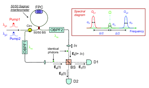
Figure 1: Schematic of the Hong-Ou-Mandel experiment with the 50/50 Sagnac-loop identical photon source. FPC, fibre polarization controller; BS, beam splitter; OBPF, optical bandpass filter; D1, D2, photon-counting detectors. Inset shows the spectral diagram of the non-degenerate pump and degenerate signal/idler fields. $\Omega_{p1}$, pump-1 ($p1$) central frequency; $\Omega_{p2}$, pump-2 ($p2$) central frequency; $\Omega$, signal/idler central frequency; $\sigma_{p}$, pump bandwidth; $\sigma_{0}$, OBPF bandwidth; $\Delta/2$, central frequency difference between P2 and signal/idler (or signal/idler and P1); $\mathbf{E_{s}}$, $\mathbf{E_{i}}$, $\mathbf{E_{1}}$ and $\mathbf{E_{2}}$, electrical fields before and after the BS, see text for details.

The degenerate signal/idler field, with a center frequency at $\Omega$, is quantized according to Grice97 :

$\displaystyle E_{s}^{(-)}$ $\displaystyle=$ βˆ«π‘‘Ο‰s​A​(Ο‰s)​as†​eβˆ’i​[k​(Ο‰s)​zβˆ’Ο‰s​t],differential-dsubscriptπœ”π‘ π΄subscriptπœ”π‘ superscriptsubscriptπ‘Žπ‘ β€ superscript𝑒𝑖delimited-[]π‘˜subscriptπœ”π‘ π‘§subscriptπœ”π‘ π‘‘\displaystyle\int d\omega_{s}\,A(\omega_{s})\,a_{s}^{{\dagger}}\,e^{-i[k(\omega_{s})z-\omega_{s}t]}\,, (4)
$\displaystyle E_{i}^{(-)}$ $\displaystyle=$ βˆ«π‘‘Ο‰i​A​(Ο‰i)​ai†​eβˆ’i​[k​(Ο‰i)​zβˆ’Ο‰i​t],differential-dsubscriptπœ”π‘–π΄subscriptπœ”π‘–superscriptsubscriptπ‘Žπ‘–β€ superscript𝑒𝑖delimited-[]π‘˜subscriptπœ”π‘–π‘§subscriptπœ”π‘–π‘‘\displaystyle\int d\omega_{i}\,A(\omega_{i})\,a_{i}^{{\dagger}}\,e^{-i[k(\omega_{i})z-\omega_{i}t]}\,, (5)

where aj†​(j=s,i)superscriptsubscriptπ‘Žπ‘—β€ π‘—π‘ π‘–a_{j}^{{\dagger}}\,(j=s,i) is the creation operator for the $j$ mode with frequency $\omega_{j}$ and wave-vector magnitude $k(\omega_{j})=\displaystyle\frac{n(\omega_{j})\,\omega_{j}}{c}$. Ο‰s=Ξ©+Ξ½ssubscriptπœ”π‘ Ξ©subscriptπœˆπ‘ \omega_{s}=\Omega+\nu_{s} and $\omega_{i}=\Omega+\nu_{i}$ represent the frequency of signal and idler photon, respectively, where Ξ½ssubscriptπœˆπ‘ \nu_{s} and $\nu_{i}$ are the deviations for each photon’s frequency from their central frequency $\Omega$. $A(\omega_{j})=-i\sqrt{\displaystyle\frac{\hbar\omega_{j}}{2\epsilon_{0}n^{2}(\omega_{j})}}$ is a slowly varying function of frequency and may be taken outside the integral. Now the interaction Hamiltonian may be expressed as

$\displaystyle H_{I}(t)$ $\displaystyle=$ Aβ€‹βˆ«βˆ’L0𝑑zβ€‹βˆ«π‘‘Ο‰sβ€‹βˆ«π‘‘Ο‰i​as†​aiβ€ β€‹βˆ«π‘‘Ο‰p​1β€‹βˆ«π‘‘Ο‰p​2​eβˆ’i​γ​(P1+P2)​z​EΒ―p​1​(Ο‰p​1)​EΒ―p​2​(Ο‰p​2)𝐴superscriptsubscript𝐿0differential-d𝑧differential-dsubscriptπœ”π‘ differential-dsubscriptπœ”π‘–superscriptsubscriptπ‘Žπ‘ β€ superscriptsubscriptπ‘Žπ‘–β€ differential-dsubscriptπœ”π‘1differential-dsubscriptπœ”π‘2superscript𝑒𝑖𝛾subscript𝑃1subscript𝑃2𝑧subscript¯𝐸𝑝1subscriptπœ”π‘1subscript¯𝐸𝑝2subscriptπœ”π‘2\displaystyle A\int_{-L}^{0}dz\int d\omega_{s}\int d\omega_{i}\,a_{s}^{{\dagger}}\,a_{i}^{{\dagger}}\int d\omega_{p1}\int d\omega_{p2}\,e^{-i\gamma(P_{1}+P_{2})z}\,\overline{E}_{p1}(\omega_{p1})\,\overline{E}_{p2}(\omega_{p2}) (6)
exp​{i​[k​(Ο‰p​1)+k​(Ο‰p​2)βˆ’k​(Ο‰s)βˆ’k​(Ο‰i)]​zβˆ’i​(Ο‰p​1+Ο‰p​2βˆ’Ο‰sβˆ’Ο‰i)​t},exp𝑖delimited-[]π‘˜subscriptπœ”π‘1π‘˜subscriptπœ”π‘2π‘˜subscriptπœ”π‘ π‘˜subscriptπœ”π‘–π‘§π‘–subscriptπœ”π‘1subscriptπœ”π‘2subscriptπœ”π‘ subscriptπœ”π‘–π‘‘\displaystyle{\rm exp}\{i[k(\omega_{p1})+k(\omega_{p2})-k(\omega_{s})-k(\omega_{i})]z-i(\omega_{p1}+\omega_{p2}-\omega_{s}-\omega_{i})t\}\,,

where $L$ is the length of the fiber, and $A$ is an overall constant consisting of $\alpha$, $A(\omega_{j})$ and the effective cross-section of the fiber $A_{\rm eff}$.

The state vector at the output of the fiber can be calculated by means of first-order perturbation theory, namely,

$\displaystyle|\Psi\rangle_{\rm out}$ $\displaystyle=$ $\displaystyle|0\rangle+\frac{1}{i\,\hbar}\int_{-\infty}^{\infty}H_{I}(t)\,dt\,|0\rangle\,,$ (7)

where the second term is the two-photon state that we seek, which we denote simply by $|\Psi\rangle$. After taking into account the fact that

βˆ«βˆ’βˆžβˆžeβˆ’i​(Ο‰p​1+Ο‰p​2βˆ’Ο‰sβˆ’Ο‰i)​t​𝑑tsuperscriptsubscriptsuperscript𝑒𝑖subscriptπœ”π‘1subscriptπœ”π‘2subscriptπœ”π‘ subscriptπœ”π‘–π‘‘differential-d𝑑\displaystyle\int_{-\infty}^{\infty}e^{-i(\omega_{p1}+\omega_{p2}-\omega_{s}-\omega_{i})t}dt $\displaystyle=$ 2​π​δ​(Ο‰p​1+Ο‰p​2βˆ’Ο‰sβˆ’Ο‰i),2πœ‹π›Ώsubscriptπœ”π‘1subscriptπœ”π‘2subscriptπœ”π‘ subscriptπœ”π‘–\displaystyle 2\pi\delta(\omega_{p1}+\omega_{p2}-\omega_{s}-\omega_{i})\,, (8)

we arrive at the following expression of the two-photon state:

$\displaystyle|\Psi\rangle$ $\displaystyle=$ 2​π​Aiβ€‹β„β€‹βˆ«βˆ’L0𝑑zβ€‹βˆ«π‘‘Ο‰sβ€‹βˆ«π‘‘Ο‰i​as†​ai†​|0βŸ©β€‹βˆ«π‘‘Ο‰p​1​eβˆ’i​γ​(P1+P2)​z2πœ‹π΄π‘–Planck-constant-over-2-pisuperscriptsubscript𝐿0differential-d𝑧differential-dsubscriptπœ”π‘ differential-dsubscriptπœ”π‘–superscriptsubscriptπ‘Žπ‘ β€ superscriptsubscriptπ‘Žπ‘–β€ ket0differential-dsubscriptπœ”π‘1superscript𝑒𝑖𝛾subscript𝑃1subscript𝑃2𝑧\displaystyle\frac{2\pi A}{i\hbar}\,\int_{-L}^{0}dz\int d\omega_{s}\int d\omega_{i}\,a_{s}^{{\dagger}}\,a_{i}^{{\dagger}}|0\rangle\,\int d\omega_{p1}\,e^{-i\gamma(P_{1}+P_{2})z} (9)
EΒ―p​1​(Ο‰p​1)​EΒ―p​2​(Ο‰s+Ο‰iβˆ’Ο‰p​1)​ei​[k​(Ο‰p​1)+k​(Ο‰s+Ο‰iβˆ’Ο‰p​1)βˆ’k​(Ο‰s)βˆ’k​(Ο‰i)]​zsubscript¯𝐸𝑝1subscriptπœ”π‘1subscript¯𝐸𝑝2subscriptπœ”π‘ subscriptπœ”π‘–subscriptπœ”π‘1superscript𝑒𝑖delimited-[]π‘˜subscriptπœ”π‘1π‘˜subscriptπœ”π‘ subscriptπœ”π‘–subscriptπœ”π‘1π‘˜subscriptπœ”π‘ π‘˜subscriptπœ”π‘–π‘§\displaystyle\overline{E}_{p1}(\omega_{p1})\,\overline{E}_{p2}(\omega_{s}+\omega_{i}-\omega_{p1})\,e^{i[k(\omega_{p1})+k(\omega_{s}+\omega_{i}-\omega_{p1})-k(\omega_{s})-k(\omega_{i})]z}

where we have utilized the $\delta$-function to simplify the integral over $\omega_{p2}$, which also reinforces the energy conservation among the four interacting optical fields.

To further simplify our analysis, we refer to the inset β€œSpectral diagram” shown in Fig.Β 1, which clearly illustrates the various system parameters by their corresponding mathematical symbols. These parameters correspond to the experimental settings schematically depicted in the main part of Fig.Β 1. The two pump pulses are both assumed to be Gaussian-shaped with equal amplitude and equal bandwidth, i.e.,

$\displaystyle\overline{E}_{p1}(\omega)$ $\displaystyle=$ $\displaystyle E_{p}\,e^{-\frac{(\omega-\Omega_{p1})^{2}}{2\sigma_{p}^{2}}}\,,$
$\displaystyle\overline{E}_{p2}(\omega)$ $\displaystyle=$ $\displaystyle E_{p}\,e^{-\frac{(\omega-\Omega_{p2})^{2}}{2\sigma_{p}^{2}}}\,,$ (10)

where $P_{1}=P_{2}\equiv P_{p}\propto E_{p}^{2}\,\sigma_{p}^{2}$ are the peak powers of the two pump pulses, and $\sigma_{p}$ denotes their common optical bandwidth. By using Taylor expansion at the frequency $\Omega$ for the various $k$’s, we obtain

$\displaystyle\Delta k$ $\displaystyle\equiv$ k​(Ο‰p​1)+k​(Ο‰s+Ο‰iβˆ’Ο‰p​1)βˆ’k​(Ο‰s)βˆ’k​(Ο‰i)π‘˜subscriptπœ”π‘1π‘˜subscriptπœ”π‘ subscriptπœ”π‘–subscriptπœ”π‘1π‘˜subscriptπœ”π‘ π‘˜subscriptπœ”π‘–\displaystyle k(\omega_{p1})+k(\omega_{s}+\omega_{i}-\omega_{p1})-k(\omega_{s})-k(\omega_{i}) (11)
$\displaystyle=$ k′′​(Ξ©)​[(Ξ”2βˆ’Ξ½p)2+(Ξ”2βˆ’Ξ½p)​(Ξ½s+Ξ½i)+Ξ½s​νi],superscriptπ‘˜β€²β€²Ξ©delimited-[]superscriptΞ”2subscriptπœˆπ‘2Ξ”2subscriptπœˆπ‘subscriptπœˆπ‘ subscriptπœˆπ‘–subscriptπœˆπ‘ subscriptπœˆπ‘–\displaystyle k^{\prime\prime}(\Omega)\left[\left(\frac{\Delta}{2}-\nu_{p}\right)^{2}+\left(\frac{\Delta}{2}-\nu_{p}\right)\left(\nu_{s}+\nu_{i}\right)+\nu_{s}\,\nu_{i}\right]\,,

where we keep the expansion series to second-order dispersion only, which proves to be sufficient in most cases.

The $\omega_{p1}$-integral in Eq.Β (9) can be rewritten as

Φ​(Ξ½s,Ξ½i,z)Ξ¦subscriptπœˆπ‘ subscriptπœˆπ‘–π‘§\displaystyle\Phi(\nu_{s},\nu_{i},z) $\displaystyle\equiv$ βˆ«π‘‘Ο‰p​1​EΒ―p​1​(Ο‰p​1)​EΒ―p​2​(Ο‰s+Ο‰iβˆ’Ο‰p​1)​ei​Δ​k​zdifferential-dsubscriptπœ”π‘1subscript¯𝐸𝑝1subscriptπœ”π‘1subscript¯𝐸𝑝2subscriptπœ”π‘ subscriptπœ”π‘–subscriptπœ”π‘1superscriptπ‘’π‘–Ξ”π‘˜π‘§\displaystyle\int d\omega_{p1}\overline{E}_{p1}(\omega_{p1})\,\overline{E}_{p2}(\omega_{s}+\omega_{i}-\omega_{p1})\,e^{i\Delta kz} (12)
$\displaystyle=$ Ep2β€‹βˆ«π‘‘Ξ½p​eβˆ’Ξ½p2+(Ξ½s+Ξ½iβˆ’Ξ½p)22​σp2+i​β2​z​[(Ξ”2βˆ’Ξ½p)2+(Ξ”2βˆ’Ξ½p)​(Ξ½s+Ξ½i)+Ξ½s​νi],superscriptsubscript𝐸𝑝2differential-dsubscriptπœˆπ‘superscript𝑒superscriptsubscriptπœˆπ‘2superscriptsubscriptπœˆπ‘ subscriptπœˆπ‘–subscriptπœˆπ‘22superscriptsubscriptπœŽπ‘2𝑖subscript𝛽2𝑧delimited-[]superscriptΞ”2subscriptπœˆπ‘2Ξ”2subscriptπœˆπ‘subscriptπœˆπ‘ subscriptπœˆπ‘–subscriptπœˆπ‘ subscriptπœˆπ‘–\displaystyle E_{p}^{2}\int d\nu_{p}\,e^{-\frac{\nu_{p}^{2}+(\nu_{s}+\nu_{i}-\nu_{p})^{2}}{2\sigma_{p}^{2}}+i\beta_{2}z\left[\left(\frac{\Delta}{2}-\nu_{p}\right)^{2}+\left(\frac{\Delta}{2}-\nu_{p}\right)\left(\nu_{s}+\nu_{i}\right)+\nu_{s}\,\nu_{i}\right]}\,,

where in the last step we have used Eqs.Β (10) and (11), and $\beta_{2}$ is a shorthand for $k^{\prime\prime}(\Omega)$. We are then left with the length integral

Q​(Ξ½s,Ξ½i)𝑄subscriptπœˆπ‘ subscriptπœˆπ‘–\displaystyle Q(\nu_{s},\nu_{i}) $\displaystyle\equiv$ βˆ«βˆ’L0𝑑z​Φ​(Ξ½s,Ξ½i,z)​eβˆ’2​i​γ​Pp​z,superscriptsubscript𝐿0differential-d𝑧Φsubscriptπœˆπ‘ subscriptπœˆπ‘–π‘§superscript𝑒2𝑖𝛾subscript𝑃𝑝𝑧\displaystyle\int_{-L}^{0}dz\,\Phi(\nu_{s},\nu_{i},z)\,e^{-2i\gamma P_{p}z}\,, (13)

and the two-photon state in Eq.Β (9) is reorganized into

$\displaystyle|\Psi\rangle$ $\displaystyle=$ 2​π​Aiβ€‹β„β€‹βˆ«π‘‘Ξ½sβ€‹βˆ«π‘‘Ξ½i​Q​(Ξ½s,Ξ½i)​|Ξ©+Ξ½sβŸ©β€‹|Ξ©+Ξ½i⟩,2πœ‹π΄π‘–Planck-constant-over-2-pidifferential-dsubscriptπœˆπ‘ differential-dsubscriptπœˆπ‘–π‘„subscriptπœˆπ‘ subscriptπœˆπ‘–ketΞ©subscriptπœˆπ‘ ketΞ©subscriptπœˆπ‘–\displaystyle\frac{2\pi A}{i\hbar}\int d\nu_{s}\int d\nu_{i}\,Q(\nu_{s},\nu_{i})|\Omega+\nu_{s}\rangle|\Omega+\nu_{i}\rangle\,, (14)

where $|\omega\rangle$ is a one-photon Fock state populated with a single photon of frequency $\omega$. We remark that the function Q​(Ξ½s,Ξ½i)𝑄subscriptπœˆπ‘ subscriptπœˆπ‘–Q(\nu_{s},\nu_{i}) is completely analogous to $\alpha(\omega_{o}+\omega_{e})\,\Phi(\omega_{o},\omega_{e})$ in Eq. (9) in Ref.Β Grice97 . Similarly, |Q​(Ξ½s,Ξ½i)|2superscript𝑄subscriptπœˆπ‘ subscriptπœˆπ‘–2|Q(\nu_{s},\nu_{i})|^{2} can be interpreted as the probability distribution of the two-photon stateΒ Grice97 . However, the apparent symmetry of Φ​(Ξ½s,Ξ½i,z)Ξ¦subscriptπœˆπ‘ subscriptπœˆπ‘–π‘§\Phi(\nu_{s},\nu_{i},z), and thus Q​(Ξ½s,Ξ½i)𝑄subscriptπœˆπ‘ subscriptπœˆπ‘–Q(\nu_{s},\nu_{i}), with respect to its two frequency arguments results in qualitatively different behavior for the two-photon state from that in Ref.Β Grice97 , which is asymmetric in its frequency arguments.

Further evaluation of Φ​(Ξ½s,Ξ½i,z)Ξ¦subscriptπœˆπ‘ subscriptπœˆπ‘–π‘§\Phi(\nu_{s},\nu_{i},z) is made possible by using the integral formula from Ref.Β Gradshteyn , which deals with Gaussian integrals with complex arguments, resulting in

Φ​(Ξ½s,Ξ½i,z)Ξ¦subscriptπœˆπ‘ subscriptπœˆπ‘–π‘§\displaystyle\Phi(\nu_{s},\nu_{i},z) $\displaystyle=$ π​σp​Ep2​eβˆ’(Ξ½s+Ξ½i)24​σp2​exp​[βˆ’Ξ²22​z2​Δ2​σp24​(1+Ξ²22​z2​σp4)]1+Ξ²22​z2​σp44​exp​{i​β2​z4​[Ξ”2βˆ’(Ξ½sβˆ’Ξ½i)2]}πœ‹subscriptπœŽπ‘superscriptsubscript𝐸𝑝2superscript𝑒superscriptsubscriptπœˆπ‘ subscriptπœˆπ‘–24superscriptsubscriptπœŽπ‘2expdelimited-[]superscriptsubscript𝛽22superscript𝑧2superscriptΞ”2superscriptsubscriptπœŽπ‘241superscriptsubscript𝛽22superscript𝑧2superscriptsubscriptπœŽπ‘441superscriptsubscript𝛽22superscript𝑧2superscriptsubscriptπœŽπ‘4exp𝑖subscript𝛽2𝑧4delimited-[]superscriptΞ”2superscriptsubscriptπœˆπ‘ subscriptπœˆπ‘–2\displaystyle\sqrt{\pi}\,\sigma_{p}\,E_{p}^{2}\,e^{-\frac{(\nu_{s}+\nu_{i})^{2}}{4\sigma_{p}^{2}}}\,\frac{{\rm exp}\left[-\frac{\beta_{2}^{2}\,z^{2}\,\Delta^{2}\,\sigma_{p}^{2}}{4(1+\beta_{2}^{2}\,z^{2}\,\sigma_{p}^{4})}\right]}{\sqrt[4]{1+\beta_{2}^{2}\,z^{2}\,\sigma_{p}^{4}}}\,{\rm exp}\left\{\frac{i\beta_{2}z}{4}\left[\Delta^{2}-(\nu_{s}-\nu_{i})^{2}\right]\right\} (15)
$\displaystyle{\rm exp}\left[\frac{i}{2}\,\arctan(\beta_{2}\,z\,\sigma_{p}^{2})-i\frac{\beta_{2}^{3}\,z^{3}\,\Delta^{2}\,\sigma_{p}^{4}}{4(1+\beta_{2}^{2}\,z^{2}\,\sigma_{p}^{4})}\right]\,,$

where $\Delta\equiv\Omega_{p2}-\Omega_{p1}$ is the central frequency difference between the two pump fields. We have thus formally obtained the expression for the two-photon state, which is given by Eq.Β (14) or its following alternative version:

$\displaystyle|\Psi\rangle$ $\displaystyle=$ 2​π​Aiβ€‹β„β€‹βˆ«π‘‘Ο‰sβ€‹βˆ«π‘‘Ο‰i​Q~​(Ο‰s,Ο‰i)​|Ο‰sβŸ©β€‹|Ο‰i⟩,2πœ‹π΄π‘–Planck-constant-over-2-pidifferential-dsubscriptπœ”π‘ differential-dsubscriptπœ”π‘–~𝑄subscriptπœ”π‘ subscriptπœ”π‘–ketsubscriptπœ”π‘ ketsubscriptπœ”π‘–\displaystyle\frac{2\pi A}{i\hbar}\int d\omega_{s}\int d\omega_{i}\,\widetilde{Q}(\omega_{s},\omega_{i})|\omega_{s}\rangle|\omega_{i}\rangle\,, (16)

where Q~​(Ο‰s,Ο‰i)~𝑄subscriptπœ”π‘ subscriptπœ”π‘–\widetilde{Q}(\omega_{s},\omega_{i}) is equivalent to Q​(Ο‰sβˆ’Ξ©,Ο‰iβˆ’Ξ©)𝑄subscriptπœ”π‘ Ξ©subscriptπœ”π‘–Ξ©Q(\omega_{s}-\Omega,\omega_{i}-\Omega) given by Eq.Β (13).

After obtaining the two-photon state, we are now ready to analyze the experiment shown schematically in Fig.Β 1. A variable delay $\delta\tau$ is inserted in one photon’s path, before the two identical photons are recombined at the 50/50 beam-splitter (BS). As shown in Fig.Β 1, if we denote the electric-field operators before the BS as $E_{s}^{(+)}(t)$ and $E_{i}^{(+)}(t+\delta\tau)$, then the field operators after the BS are given by

$\displaystyle E_{1}^{(+)}(t)$ $\displaystyle=$ $\displaystyle\frac{1}{\sqrt{2}}\left[E_{s}^{(+)}(t)+iE_{i}^{(+)}(t+\delta\tau)\right]\,,$
$\displaystyle E_{2}^{(+)}(t)$ $\displaystyle=$ $\displaystyle\frac{1}{\sqrt{2}}\left[iE_{s}^{(+)}(t)+E_{i}^{(+)}(t+\delta\tau)\right]\,,$ (17)

where the vector nature of the field operators are ignored since they all share the same polarization, and

Es,i(+)​(t)βˆβˆ«π‘‘Ο‰s,i​as,i​(Ο‰s,i)​eβˆ’i​ωs,i​t​eβˆ’(Ο‰s,iβˆ’Ξ©)22​σ02proportional-tosuperscriptsubscript𝐸𝑠𝑖𝑑differential-dsubscriptπœ”π‘ π‘–subscriptπ‘Žπ‘ π‘–subscriptπœ”π‘ π‘–superscript𝑒𝑖subscriptπœ”π‘ π‘–π‘‘superscript𝑒superscriptsubscriptπœ”π‘ π‘–Ξ©22superscriptsubscript𝜎02\displaystyle E_{s,i}^{(+)}(t)\propto\int d\omega_{s,i}\,a_{s,i}(\omega_{s,i})\,e^{-i\omega_{s,i}t}\,e^{-\frac{(\omega_{s,i}-\Omega)^{2}}{2\sigma_{0}^{2}}} (18)

are the electric-field operators before the BS that include the shape of the OBPF, which is assumed to be Gaussian here. The coincidence-count rate registered by detectors D1 and D2 is given byΒ Glauber

$\displaystyle R_{c}(\delta\tau)$ $\displaystyle=$ $\displaystyle\int_{0}^{\infty}dt_{1}\int_{0}^{\infty}dt_{2}\,P_{12}(t_{1},t_{2},\delta\tau)\,,$ (19)

where

$\displaystyle P_{12}(t_{1},t_{2},\delta\tau)$ $\displaystyle=$ $\displaystyle\langle\Psi|E_{1}^{(-)}(t_{1})E_{2}^{(-)}(t_{2})E_{2}^{(+)}(t_{2})E_{1}^{(+)}(t_{1})|\Psi\rangle$ (20)
$\displaystyle=$ $\displaystyle|\langle 0|E_{2}^{(+)}(t_{2})E_{1}^{(+)}(t_{1})|\Psi\rangle|^{2}$

is the probability per pulse for coincidence detection between the two detectors.

Eqs.Β (16), (17), (18), and (20), when plugged into Eq.Β (19), after a simple but lengthy calculation, yield

$\displaystyle R_{c}(\delta\tau)$ $\displaystyle\propto$ βˆ«π‘‘Ο‰sβ€‹βˆ«π‘‘Ο‰i​|F~​(Ο‰s,Ο‰i)|2​[1βˆ’eβˆ’i​(Ο‰iβˆ’Ο‰s)​δ​τ],differential-dsubscriptπœ”π‘ differential-dsubscriptπœ”π‘–superscript~𝐹subscriptπœ”π‘ subscriptπœ”π‘–2delimited-[]1superscript𝑒𝑖subscriptπœ”π‘–subscriptπœ”π‘ π›Ώπœ\displaystyle\int d\omega_{s}\int d\omega_{i}\,|\widetilde{F}(\omega_{s},\omega_{i})|^{2}\,\left[1-e^{-i(\omega_{i}-\omega_{s})\delta\tau}\right]\,,
F~​(Ο‰s,Ο‰i)~𝐹subscriptπœ”π‘ subscriptπœ”π‘–\displaystyle\widetilde{F}(\omega_{s},\omega_{i}) $\displaystyle=$ Q~​(Ο‰s,Ο‰i)​exp​[βˆ’(Ο‰sβˆ’Ξ©)22​σ02βˆ’(Ο‰iβˆ’Ξ©)22​σ02],~𝑄subscriptπœ”π‘ subscriptπœ”π‘–expdelimited-[]superscriptsubscriptπœ”π‘ Ξ©22superscriptsubscript𝜎02superscriptsubscriptπœ”π‘–Ξ©22superscriptsubscript𝜎02\displaystyle\widetilde{Q}(\omega_{s},\omega_{i})\,{\rm exp}\left[-\frac{(\omega_{s}-\Omega)^{2}}{2\sigma_{0}^{2}}-\frac{(\omega_{i}-\Omega)^{2}}{2\sigma_{0}^{2}}\right]\,, (21)

where we have used the fact that F~​(Ο‰s,Ο‰i)=F~​(Ο‰i,Ο‰s)~𝐹subscriptπœ”π‘ subscriptπœ”π‘–~𝐹subscriptπœ”π‘–subscriptπœ”π‘ \widetilde{F}(\omega_{s},\omega_{i})=\widetilde{F}(\omega_{i},\omega_{s}) in obtaining the above results111We remark that, in the case of F~​(Ο‰s,Ο‰i)β‰ F~​(Ο‰i,Ο‰s)~𝐹subscriptπœ”π‘ subscriptπœ”π‘–~𝐹subscriptπœ”π‘–subscriptπœ”π‘ \widetilde{F}(\omega_{s},\omega_{i})\neq\widetilde{F}(\omega_{i},\omega_{s}), we would have obtained Rc​(δ​τ)βˆβˆ«π‘‘Ο‰sβ€‹βˆ«π‘‘Ο‰i​[|F~​(Ο‰s,Ο‰i)|2βˆ’F~​(Ο‰s,Ο‰i)​F~βˆ—β€‹(Ο‰i,Ο‰s)​eβˆ’i​(Ο‰iβˆ’Ο‰s)​δ​τ]proportional-tosubscriptπ‘…π‘π›Ώπœdifferential-dsubscriptπœ”π‘ differential-dsubscriptπœ”π‘–delimited-[]superscript~𝐹subscriptπœ”π‘ subscriptπœ”π‘–2~𝐹subscriptπœ”π‘ subscriptπœ”π‘–superscript~𝐹subscriptπœ”π‘–subscriptπœ”π‘ superscript𝑒𝑖subscriptπœ”π‘–subscriptπœ”π‘ π›ΏπœR_{c}(\delta\tau)\propto\int d\omega_{s}\int d\omega_{i}\,\left[|\widetilde{F}(\omega_{s},\omega_{i})|^{2}-\widetilde{F}(\omega_{s},\omega_{i})\,\widetilde{F}^{*}(\omega_{i},\omega_{s})\,e^{-i(\omega_{i}-\omega_{s})\delta\tau}\right].. Its alternative version, written in terms of the difference-frequency Ξ½ssubscriptπœˆπ‘ \nu_{s} and $\nu_{i}$, reads

$\displaystyle R_{c}(\delta\tau)$ $\displaystyle\propto$ βˆ«π‘‘Ξ½sβ€‹βˆ«π‘‘Ξ½i​|F​(Ξ½s,Ξ½i)|2​[1βˆ’eβˆ’i​(Ξ½iβˆ’Ξ½s)​δ​τ],differential-dsubscriptπœˆπ‘ differential-dsubscriptπœˆπ‘–superscript𝐹subscriptπœˆπ‘ subscriptπœˆπ‘–2delimited-[]1superscript𝑒𝑖subscriptπœˆπ‘–subscriptπœˆπ‘ π›Ώπœ\displaystyle\int d\nu_{s}\int d\nu_{i}\,|F(\nu_{s},\nu_{i})|^{2}\,\left[1-e^{-i(\nu_{i}-\nu_{s})\delta\tau}\right]\,,
F​(Ξ½s,Ξ½i)𝐹subscriptπœˆπ‘ subscriptπœˆπ‘–\displaystyle F(\nu_{s},\nu_{i}) $\displaystyle=$ Q​(Ξ½s,Ξ½i)​exp​(βˆ’Ξ½s2+Ξ½i22​σ02).𝑄subscriptπœˆπ‘ subscriptπœˆπ‘–expsuperscriptsubscriptπœˆπ‘ 2superscriptsubscriptπœˆπ‘–22superscriptsubscript𝜎02\displaystyle Q(\nu_{s},\nu_{i})\,{\rm exp}\left(-\frac{\nu_{s}^{2}+\nu_{i}^{2}}{2\sigma_{0}^{2}}\right)\,. (22)

It turns out that further simplification is possible for the above Gaussian-filter case (by using again the formula from Ref.Β Gradshteyn ), which we explicitly write out as the following:

$\displaystyle R_{c}(\delta\tau)$ $\displaystyle\propto$ $\displaystyle\int_{-L}^{0}dz_{1}\int_{-L}^{0}dz_{2}\,G(z_{1})\,G^{*}(z_{2})\,I(z_{1},z_{2})\,,$ (23)
$\displaystyle G(z)$ $\displaystyle=$ $\displaystyle\frac{{\rm exp}\left[-\frac{\beta_{2}^{2}\,z^{2}\,\Delta^{2}\,\sigma_{p}^{2}}{4(1+\beta_{2}^{2}\,z^{2}\,\sigma_{p}^{4})}\right]}{\sqrt[4]{1+\beta_{2}^{2}\,z^{2}\,\sigma_{p}^{4}}}\,{\rm exp}\left[\frac{i}{2}\,\arctan(\beta_{2}\,z\,\sigma_{p}^{2})\right]$ (24)
$\displaystyle{\rm exp}\left[-i\frac{\beta_{2}^{3}\,z^{3}\,\Delta^{2}\,\sigma_{p}^{4}}{4(1+\beta_{2}^{2}\,z^{2}\,\sigma_{p}^{4})}\right]\,{\rm exp}\left[i\frac{\beta_{2}\,\Delta^{2}\,z}{4}-2i\gamma P_{p}z\right]\,,$
$\displaystyle I(z_{1},z_{2})$ $\displaystyle=$ $\displaystyle\frac{\sqrt{2}\,\pi^{2}\,P_{p}^{2}\,\sigma_{0}^{2}}{\sigma_{p}\,\sqrt{\sigma_{p}^{2}+\sigma_{0}^{2}}}\,\frac{{\rm exp}\left\{\frac{i}{2}\,\arctan\left[-\frac{\beta_{2}\,(z_{1}-z_{2})\,\sigma_{0}^{2}}{2}\right]\right\}}{\sqrt[4]{4+\beta_{2}^{2}\,(z_{1}-z_{2})^{2}\,\sigma_{0}^{4}}}$ (25)
$\displaystyle\left\{1-{\rm exp}\left[-\frac{2\,\delta\tau^{2}\,\sigma_{0}^{2}}{4+\beta_{2}^{2}\,(z_{1}-z_{2})^{2}\,\sigma_{0}^{4}}+i\frac{\beta_{2}\,(z_{1}-z_{2})\,\delta\tau^{2}\,\sigma_{0}^{4}}{4+\beta_{2}^{2}\,(z_{1}-z_{2})^{2}\,\sigma_{0}^{4}}\right]\right\}\,.$

One can, for instance, generalize the above result to investigate the effect that the filter has on the Hong-Ou-Mandel (HOM) dip. Due to its experimental relevance, we shall write out explicitly the formula that describes the case when the previously Gaussian-shaped OBPFs are replaced with two identical super-Gaussian filters, which reads

$\displaystyle R_{c}(\delta\tau)$ $\displaystyle\propto$ π​Pp2Οƒp2β€‹βˆ«βˆ’L0𝑑z1β€‹βˆ«βˆ’L0𝑑z2β€‹βˆ«π‘‘Ξ½sβ€‹βˆ«π‘‘Ξ½i​G​(z1)​Gβˆ—β€‹(z2)​eβˆ’(Ξ½s+Ξ½i)22​σp2​eβˆ’Ξ½s4+Ξ½i4Οƒ04πœ‹superscriptsubscript𝑃𝑝2superscriptsubscriptπœŽπ‘2superscriptsubscript𝐿0differential-dsubscript𝑧1superscriptsubscript𝐿0differential-dsubscript𝑧2differential-dsubscriptπœˆπ‘ differential-dsubscriptπœˆπ‘–πΊsubscript𝑧1superscript𝐺subscript𝑧2superscript𝑒superscriptsubscriptπœˆπ‘ subscriptπœˆπ‘–22superscriptsubscriptπœŽπ‘2superscript𝑒superscriptsubscriptπœˆπ‘ 4superscriptsubscriptπœˆπ‘–4superscriptsubscript𝜎04\displaystyle\frac{\pi\,P_{p}^{2}}{\sigma_{p}^{2}}\int_{-L}^{0}dz_{1}\int_{-L}^{0}dz_{2}\int d\nu_{s}\int d\nu_{i}\,G(z_{1})\,G^{*}(z_{2})\,e^{-\frac{(\nu_{s}+\nu_{i})^{2}}{2\sigma_{p}^{2}}}\,e^{-\frac{\nu_{s}^{4}+\nu_{i}^{4}}{\sigma_{0}^{4}}} (26)
exp​[βˆ’i​β24​(Ξ½sβˆ’Ξ½i)2​(z1βˆ’z2)]​[1βˆ’eβˆ’i​(Ξ½iβˆ’Ξ½s)​δ​τ],expdelimited-[]𝑖subscript𝛽24superscriptsubscriptπœˆπ‘ subscriptπœˆπ‘–2subscript𝑧1subscript𝑧2delimited-[]1superscript𝑒𝑖subscriptπœˆπ‘–subscriptπœˆπ‘ π›Ώπœ\displaystyle{\rm exp}\left[-i\frac{\beta_{2}}{4}(\nu_{s}-\nu_{i})^{2}(z_{1}-z_{2})\right]\,\left[1-e^{-i(\nu_{i}-\nu_{s})\delta\tau}\right]\,,

where $G(z)$ is given by Eq.Β (24).

Refer to caption

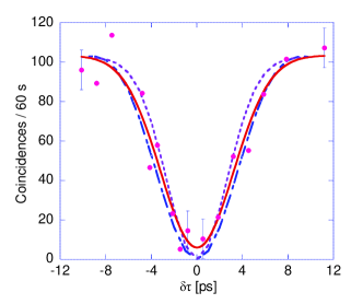
Figure 2: Theoretical predictions vs. experimental results. Pink filled circles, experimental data; red solid curve, least-square fitting for the data; purple dotted curve, theory fitting from Eq.Β (23) for Gaussian OBPFs; blue dot-dashed curve, theory fitting from Eq.Β (26) for super-Gaussian OBPFs. Realistic values for the experimental parameters used in generating these curves are: $L=300$ m, $\beta_{2}=-0.116\,{\rm ps}^{2}/{\rm km}$, $\gamma=1.8\times 10^{-3}\,{\rm W}^{-1}\,{\rm m}^{-1}$, $P_{p}=0.36$ W, $c=3\times 10^{8}$ m/s, $\lambda_{p1}=1555.92$ nm, $\lambda_{p2}=1545.95$ nm, pump FWHM = 0.8 nm, signal/idler FWHM = 0.8 nm.

We then generate two curves, from both Eq.Β (23) and Eq.Β (26), to fit the experimental data obtained in the main text. The fitting results are shown in Fig.Β 2. As can be seen from the figure, both curves (blue dot-dashed and purple dotted) fit the experimental data remarkably well. The super-Gaussian fit appears to give a wider dip width ($\sim 8.0$ ps FWHM) as compared to the Gaussian fit’s result (FWHM dip width $\sim 6.4$ ps), which is commensurate with the fact that a super-Gaussian filter is spectrally narrower (and thus temporally wider) than its Gaussian counterpart with the same FWHM. A least-square Gaussian fit to the data (the red solid curve in Fig.Β 2), generated by the data-processing program, suggests that the HOM-dip visibility is $\sim 94.3\%$. It has a FWHM dip width of about 7.2 ps, which is right in between the previous two fitting values. This may be explained by the fact that the real OBPF employed in the experiment is constructed by a cascade of a Gaussian filter and a super-Gaussian one, making its transmission spectrum somewhere in between. In contrast, the two theoretical fits agree on the ideally attainable dip visibility of 100%. This result also coincides with the theoretical understanding from Ref.Β Grice97 that, as long as the two-photon probability distribution function222The term is used loosely here to refers to F​(Ξ½s,Ξ½i)𝐹subscriptπœˆπ‘ subscriptπœˆπ‘–F(\nu_{s},\nu_{i}) in our $\chi^{(3)}$ case. is symmetric with respect to its two frequency arguments, the HOM dip can achieve a maximum visibility of 100%.

Refer to caption

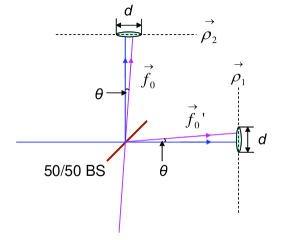
Figure 3: Schematic drawing for investigating one of the possible scenarios for the less-than-unity HOM-dip visibility: spatial mode mismatch. See text for details.

There are many reasons that could explain the missing 5.7% visibility. For example, one might wonder whether higher-order dispersion plays a role. But a straightforward Taylor expansion of the various $k$’s at the central frequency $\Omega$ [similar to Eq.Β (11)] to higher-order terms dismisses this hypothesis. In fact, the $\Delta k$ quantity is always symmetric with respect to Ξ½ssubscriptπœˆπ‘ \nu_{s} and $\nu_{i}$ in our $\chi^{(3)}$ two-photon state due to the isotropic nature of the fiber. However, a little mismatch between the two OBPFs’ spectrum will result in asymmetry of two arguments in F​(Ξ½s,Ξ½i)𝐹subscriptπœˆπ‘ subscriptπœˆπ‘–F(\nu_{s},\nu_{i}), and will certainly cause a degradation of the HOM-dip visibility. Other candidates include: (i) The real-life BS’s performance deviates from an ideal 50/50 BS, i.e., $R+T=1$ and Rβ‰ T𝑅𝑇R\neq T. This gives rises to a corrective factor of $\displaystyle\frac{2\,R\,T}{R^{2}+T^{2}}$ to the dip visibilityΒ Hong . When put in the measured values $(R=0.474,\,T=0.526)$, it gives a 99.4% corrective coefficient. (ii) There might be some remaining $\Psi_{2002}$ component due to the non-ideal alignment of the 50/50 Sagnac loop, which leads to degradation of the dip visibilityΒ Halder . (iii) The existence of other unsuppressed noise photons, such as Raman photons and single-pump FWM photons, could also degrade the attainable dip visibility. (iv) The spatial modes of the two photons are not exactly matched at the BS. A simple calculation, as we will carry out explicitly below, shows that a small angular mismatch between the two photons’ paths distinguishes between the coincidence-generating amplitudes (TT and RR). As a result, they are not completely cancelled after the BS, which correspond to the remaining coincidences at the HOM dip. An angular mismatch as small as $3\times 10^{-5}$ rad is required to bring the dip visibility down to 94.3%. The details of the calculation go as follows. Suppose at the BS the two photons intersect at a small angle $\theta$, as depicted in Fig.Β 3. The two amplitudes can each be written in the Fourier-optic language as:

$\displaystyle\psi_{\rm TT}$ $\displaystyle=$ $\displaystyle\frac{4}{\pi d^{2}}e^{i2\pi\vec{f}_{0}\cdot\vec{\rho}_{2}}\,,$
$\displaystyle\psi_{\rm RR}$ $\displaystyle=$ $\displaystyle\frac{4}{\pi d^{2}}e^{i2\pi\vec{f}^{\prime}_{0}\cdot\vec{\rho}_{1}}\,.$ (27)

Here $d$ is the diameter of the lenses used to couple light into fibre, $\vec{\rho}_{1,2}$ represent the two-dimensional coordinates at the lens planes (perpendicular to the paper), and $|\vec{f}_{0}|=|\vec{f}^{\prime}_{0}|=\frac{\sin\theta}{\lambda}$ are the projected wave-vector magnitudes in the lens planes for the two off-axis waves. The overlap between the two amplitudes, which is proportional to the HOM-dip visibilityΒ Rhode , is given by

$\displaystyle\int d\vec{\rho}_{1}\int d\vec{\rho}_{2}\,\Theta\left(\frac{2\vec{\rho}_{1}}{d}\right)\,\Theta\left(\frac{2\vec{\rho}_{2}}{d}\right)\,\left(\frac{4}{\pi d}\right)^{2}e^{-i2\pi\vec{f}_{0}\cdot\vec{\rho}_{2}}\,e^{i2\pi\vec{f}^{\prime}_{0}\cdot\vec{\rho}_{1}}$ $\displaystyle=$ $\displaystyle\left[\frac{J_{1}(\pi d|\sin\theta|/\lambda)}{\pi d|\sin\theta|/(2\lambda)}\right]^{2}$ (28)

where $\Theta(\vec{x})$ (it obtains the value 1 when $|\vec{x}|\leq 1$ and everywhere else zero) represents the effective areas of the lenses, and $J_{1}(x)$ is the first-order Bessel function. When we put in realistic values for $d=5$ mm and $\lambda=1.55$ $\mu$m, and demand that Eq.Β (28) yields 0.943, we obtain a numerical solution for $\theta\simeq\sin\theta\simeq 30\,\mu$rad. From the above calculation, we can thus see that spatial mode mismatching has the highest likelihood of contributing to the missing 5.7% HOM-dip visibility.

References

  • (1) W. P. Grice and I. A. Walmsley, β€œSpectral information and distinguishability in type-II down-conversion with a broadband pump”, Phys. Rev. A 56, 1627 (1997).
  • (2) I. S. Gradshteyn and I. M. Ryzhik, Table of integrals, series, and products, 6th ed., San Diego, CA: Academic Press 2000, where the formula of interest is (3.923).
  • (3) R. J. Glauber, β€œThe Quantum Theory of Optical Coherence”, Phys. Rev. 130, 2529 (1963).
  • (4) C. K. Hong, Z. Y. Ou, and L. Mandel, β€œMeasurement of subpicosecond time intervals between two photons by interference”, Phys. Rev. Lett. 59, 2044 (1987).
  • (5) P. P. Rhode and T. C. Ralph, β€œFrequency and temporal effects in linear optical quantum computing”, Phys. Rev. A 71, 032320 (2005).
  • (6) M. Halder, S. Tanzilli, H. de Riedmatten, A. Beveratos, H. Zbinden and N. Gisin, β€œPhoton-bunching measurement after two 25-km-long optical fibers”, Phys. Rev. A 71, 042335 (2005).