Light scattering from ultracold atoms in optical lattices as an optical probe of quantum statistics

Abstract

We study off-resonant collective light scattering from ultracold atoms trapped in an optical lattice. Scattering from different atomic quantum states creates different quantum states of the scattered light, which can be distinguished by measurements of the spatial intensity distribution, quadrature variances, photon statistics, or spectral measurements. In particular, angle-resolved intensity measurements reflect global statistics of atoms (total number of radiating atoms) as well as local statistical quantities (single-site statistics even without an optical access to a single site) and pair correlations between different sites. As a striking example we consider scattering from transversally illuminated atoms into an optical cavity mode. For the Mott insulator state, similar to classical diffraction, the number of photons scattered into a cavity is zero due to destructive interference, while for the superfluid state it is nonzero and proportional to the number of atoms. Moreover, we demonstrate that light scattering into a standing-wave cavity has a nontrivial angle dependence, including the appearance of narrow features at angles, where classical diffraction predicts zero. The measurement procedure corresponds to the quantum non-demolition (QND) measurement of various atomic variables by observing light.

I Introduction

Ever since the first generation of Bose-Einstein condensates (BEC), it has been a central task to study quantum properties of such degenerate gases. Surprisingly, it turned out that many properties are well explained by the Gross-Pitaevskii equation, which is a an effective nonlinear single-particle equation and allows to calculate the evolution of the average atomic density and phase. The density can be observed by simple absorption images after expansion, and the phase can be mapped onto density modulations in interferometric setups. The limited validity of such mean-field descriptions became apparent with the advent of optical lattices Jaksch et al. (1998); Greiner et al. (2002), where one has quantum phase transitions between states of similar average density but radically different quantum fluctuations.

The majority of methods to characterize quantum properties of degenerate gases are based on matter-wave interference between atoms released from a trap in time-of-flight measurements Greiner et al. (2002); Fölling et al. (2005); Altman et al. (2004), which destroys the system. Recently, a method of “Bragg spectroscopy” based on stimulated scattering of matter waves by laser pulses was applied to homogeneous BECs Stenger et al. (1999); Blakie et al. (2002) and atoms in lattices Roth and Burnett (2003); Stöferle et al. (2004); Menotti et al. (2003); Rey et al. (2005). In this case, the measured quantities (e.g. structure factor), which carry information about density fluctuations, are also accessible via matter-wave interference. Although the scattered light and stimulated matter waves can be entangled and mutually carry the statistical information Moore et al. (1999); Pu et al. (2003), the laser fields are simply considered as a tool to stimulate matter waves.

In contrast to those works, the nondestructive methods based on measurements of light fields only, without destroying atoms, were proposed in Refs. You et al. (1995); Idziaszek et al. (2000); Müstecaplioglu and You (2000, 2001); Javanainen (1995); Javanainen and Ruostekoski (1995); Cirac et al. (1994a, b); Saito and Ueda (1999); Prataviera and de Oliveira (2004) for homogeneous BECs in traps and optical lattices Javanainen and Ruostekoski (2003). Here the average amplitude of the scattered light is solely determined by the average atomic density, while the photon number and other higher order field expectation values contain quantum statistical properties of atoms.

In this paper, we show that this is of even greater significance for atoms in lattices, where different quantum phases show qualitatively distinct light scattering. Here we extend the preliminary results presented in our previous letter, Ref. PRL . In particular, linear scattering can create entangled states of light and manybody atomic states, exhibiting a nontrivial connection of the field amplitude and intensity. As a practical consequence, we demonstrate the possibility to distinguish between different quantum phases, e.g., Mott insulator (MI) and superfluid (SF), by measuring properties of a scattered off-resonant beam. This possibility is exhibited in several different ways involving simple intensity measurements, or more involved measurements of quadrature variances, photon statistics, as well as phase-sensitive or spectral measurements. A careful analysis of the scattered light provides information about global statistics (related to atom number at a lattice region illuminated by the probe), local quantities (reflecting statistics at a single site even without an optical single-site access), and pair correlations between different sites.

Note that we consider off-resonant and almost nondestructive light scattering, corresponding to the quantum non-demolition (QND) measurements of various atom-number functions. In principle, it can be repeatedly or even continuously applied to the same sample. This is very different from noise spectroscopy in absorption images Fölling et al. (2005) where observations of quantum fluctuations of the atomic density were recently reported.

For homogeneous BECs You et al. (1995); Idziaszek et al. (2000); Müstecaplioglu and You (2000, 2001); Javanainen (1995); Javanainen and Ruostekoski (1995); Cirac et al. (1994a, b); Saito and Ueda (1999); Prataviera and de Oliveira (2004), the scattered light was shown to consist of two contributions: the strong classical part insensitive to atomic fluctuations, and weaker one, which carries information about atom statistics. For a large atom number, the classical part completely dominates the second one, which, in some papers, even led to a conclusion about the impossibility of distinguishing between different atomic states by intensity measurements, and, hence, to a necessity to measure photon statistics.

In our work, we show that light scattering from atoms in optical lattices has essentially different and advantageous characteristics in contrast to scattering from homogeneous BECs. For example, the problem of suppressing the strong classical part of scattering has a natural solution: in the directions of classical diffraction minima, the expectation value of the light amplitude is zero, while the intensity (photon number) is nonzero and therefore directly reflects density fluctuations. Furthermore, in an optical lattice, the signal is sensitive not only to the periodic density distribution, but also to the periodic distribution of density fluctuations, giving an access to even very small nonlocal pair correlations, which is possible by measuring light in the directions of diffraction maxima.

As free space light scattering from a small sample can be weak, it might be selectively enhanced by a cavity. The corresponding light scattering from an optical lattice exhibits a complicated angle dependence and narrow angle-resolved features appear at angles, where classical diffraction cannot exist. In experiments, such a nontrivial angle dependence can help in the separation between the signal reflecting atom statistics from a technical noise.

Joining the paradigms of two broad fields of quantum physics, cavity quantum electrodynamics (QED) and ultracold gases, will enable new investigations of both light and matter at ultimate quantum levels, which only recently became experimentally possible Bourdel et al. (2006); Teper et al. (2006); Reichel . Here we predict effects accessible in such novel setups.

Experimentally, diffraction (Bragg scattering) of light from classical atoms in optical lattices was considered, for example, in Refs. Birkl et al. (1995); Weidemüller et al. (1995); Slama et al. (2006). In our work, we are essentially focused on the properties of scattering from ultracold lattice atoms with quantized center-of-mass motion.

The paper is organized as follows. In Sec. II, a general theoretical model of light scattering from atoms in an optical lattice is developed taking into account atom tunneling between neighboring sites. In Sec. III, we significantly reduce the model to the case of a deep lattice and give a classical analogy of light diffraction on a quantum lattice. Section IV presents a relation between atom statistics and different characteristics of scattered light: intensity and amplitude, quadratures, photon statistics, and phase-sensitive and spectral characteristics. Properties of different atomic states are summarized in Sec. V.

In Sec. VI, we present a simple example of the model developed: light scattering from a lattice in an optical cavity pumped orthogonally to the axis. The main results are discussed in Sec. VII and summarized in Sec. VIII.

II General model

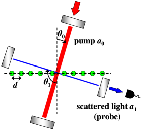
Figure 1: (Color online) Setup. Atoms in a lattice are illuminated by a pump wave at angle $\theta_{0}$; scattered (probe) light is collected by a cavity at angle $\theta_{1}$ and measured by a detector.

We consider an ensemble of $N$ two-level atoms in an optical lattice with $M$ sites. Except the presence of a trapping lattice potential, atoms are illuminated by and scatter field modes at different directions. A possible experimental realization is shown in Fig. 1. Here, a lattice is illuminated by a “pump” beam, whereas measurements are carried out in one of the scattered modes, which is treated as a “probe.” Note that different experimental setups are possible: the modes can be either in free space, or selected by traveling- or standing-wave cavities, or even correspond to different modes of the same cavity. For definiteness, we will consider the case, where mode functions are determined by cavities, whose axes directions can be varied with respect to the lattice axis (the simplest case of two standing-wave cavities at angles $\theta_{0}$ and $\theta_{1}$ is shown in Fig. 1). Instead of varying the angles, the mode wavelengths can be varied with respect to the wavelength of a trapping beam. We also assume, that not all $M$ lattice sites are necessarily illuminated by additional modes, but some region with $K\leq M$ sites.

The manybody Hamiltonian in the second quantized form is given by

$$H=H_{f}+H_{a},$$ (1a)

$$H_{f}=\sum_{l}{\hbar\omega_{l}a^{\dagger}_{l}a_{l}}-i\hbar\sum_{l}{(\eta^{*}_{l}a_{l}-\eta_{l}a^{\dagger}_{l})},$$ (1b)

$$H_{a}=\int{d^{3}{\bf r}\Psi^{\dagger}({\bf r})H_{a1}\Psi({\bf r})}$$

$$+\frac{2\pi a_{s}\hbar^{2}}{m}\int{d^{3}{\bf r}\Psi^{\dagger}({\bf r})\Psi^{\dagger}({\bf r})\Psi({\bf r})\Psi({\bf r})}.$$ (1c)

In the field part of the Hamiltonian $H_{f}$, $a_{l}$ are the annihilation operators of light modes with the frequencies $\omega_{l}$, wave vectors ${\bf k}_{l}$, and mode functions $u_{l}({\bf r})$, which can be pumped by coherent fields with amplitudes $\eta_{l}$. In the atom part, $H_{a}$, $\Psi({\bf r})$ is the atomic matter-field operator, $a_{s}$ is the $s$-wave scattering length characterizing the direct interatomic interaction, and $H_{a1}$ is the atomic part of the single-particle Hamiltonian $H_{1}$, which in the rotating-wave and dipole approximation has a form

$$H_{1}=H_{f}+H_{a1},$$ (2a)

$$H_{a1}=\frac{{\bf p}^{2}}{2m_{a}}+\frac{\hbar\omega_{a}}{2}\sigma_{z}-i\hbar g_{0}\sum_{l}{[\sigma^{+}a_{l}u_{l}({\bf r})-\text{H. c.}}]$$ (2b)

Here, ${\bf p}$ and ${\bf r}$ are the momentum and position operators of an atom of mass $m_{a}$ and resonance frequency $\omega_{a}$, $\sigma^{+}$, $\sigma^{-}$, and $\sigma_{z}$ are the raising, lowering, and population difference operators, $g_{0}$ is the atom–light coupling constant.

We will consider essentially nonresonant interaction where the light-atom detunings $\Delta_{la}=\omega_{l}-\omega_{a}$ are much larger than the spontaneous emission rate and Rabi frequencies $g_{0}a_{l}$. Thus, in the Heisenberg equations obtained from the single-atom Hamiltonian $H_{1}$ (2), $\sigma_{z}$ can be set to $-1$ (approximation of linear dipoles). Moreover, the polarization $\sigma^{-}$ can be adiabatically eliminated and expressed via the fields $a_{l}$. An effective single-particle Hamiltonian that gives the corresponding Heisenberg equation for $a_{l}$ can be written as $H_{1\text{eff}}=H_{f}+H_{a1}$ with

$$H_{a1}=\frac{{\bf p}^{2}}{2m_{a}}+V_{\text{cl}}({\bf r})+\hbar g^{2}_{0}\sum_{l,m}{\frac{u_{l}^{*}({\bf r})u_{m}({\bf r})a^{\dagger}_{l}a_{m}}{\Delta_{ma}}}.$$ (3)

Here, we have also added a classical trapping potential of the lattice, $V_{\text{cl}}({\bf r})$, corresponds to a strong classical standing wave. This potential can be, of course, derived from one of the modes $a_{l}=a_{\text{cl}}$ [in this case $V_{\text{cl}}({\bf r})=\hbar g^{2}_{0}|a_{\text{cl}}u_{\text{cl}}({\bf r})|^{2}/\Delta_{\text{cl}a}$], and it can scatter light into other modes. Nevertheless, at this point we will consider $V_{\text{cl}}({\bf r})$ as an independent potential, which does not affect light scattering of other modes that can be significantly detuned from $a_{\text{cl}}$ [i.e. the interference terms between $a_{\text{cl}}$ and other modes are not considered in the last term of Eq. (3)]. The later inclusion of the light scattered by the trapping wave will not constitute a difficulty, due to the linearity of dipoles assumed in this model.

We will consider scattering of weak modes from the atoms in a deep lattice. So, the fields $a_{l}$ are assumed much weaker than the field forming the potential $V_{\text{cl}}({\bf r})$. To derive the generalized Bose–Hubbard Hamiltonian we expand the field operator $\Psi({\bf r})$ in Eq. (1), using localized Wannier functions corresponding to $V_{\text{cl}}({\bf r})$ and keeping only the lowest vibrational state at each site: $\Psi({\bf r})=\sum_{i=1}^{M}{b_{i}w({\bf r}-{\bf r}_{i})}$, where $b_{i}$ is the annihilation operator of an atom at the site $i$ with the coordinate ${\bf r}_{i}$. Substituting this expansion in Eq. (1) with $H_{a1}$ (3), we get

$$H=H_{f}+\sum_{i,j=1}^{M}{J_{i,j}^{\text{cl}}b_{i}^{\dagger}b_{j}}+\hbar g^{2}_{0}\sum_{l,m}{\frac{a^{\dagger}_{l}a_{m}}{\Delta_{ma}}}\left(\sum_{i,j=1}^{K}{J_{i,j}^{lm}b_{i}^{\dagger}b_{j}}\right)$$

$$+\frac{U}{2}\sum_{i=1}^{M}{b_{i}^{\dagger}b_{i}(b_{i}^{\dagger}b_{i}-1)},$$ (4)

where the coefficients $J_{ij}^{\text{cl}}$ correspond to the quantum motion of atoms in the classical potential and are typical for the Bose–Hubbard Hamiltonian Jaksch et al. (1998):

$$J_{i,j}^{\text{cl}}=\int{d{\bf r}}w({\bf r}-{\bf r}_{i})\left(-\frac{\hbar^{2}\nabla^{2}}{2m}+V_{\text{cl}}({\bf r})\right)w({\bf r}-{\bf r}_{j}).$$ (5)

However, in contrast to the usual Bose–Hubbard model, one has new terms depending on the coefficients $J_{ij}^{lm}$, which describe an additional contribution arising from the presence of light modes:

$$J_{i,j}^{lm}=\int{d{\bf r}}w({\bf r}-{\bf r}_{i})u_{l}^{*}({\bf r})u_{m}({\bf r})w({\bf r}-{\bf r}_{j}).$$ (6)

In the last term of Eq. (II), only the on-site interaction was taken into account and $U=4\pi a_{s}\hbar^{2}/m_{a}\int{d{\bf r}|w({\bf r})|^{4}}$.

As a usual approximation, we consider atom tunneling being possible only to the nearest neighbor sites. Thus, coefficients (5) do not depend on the site indices ($J_{i,i}^{\text{cl}}=J_{0}^{\text{cl}}$ and $J_{i,i\pm 1}^{\text{cl}}=J^{\text{cl}}$), while coefficients (6) are still index-dependent. The Hamiltonian (II) then reads

$$H=H_{f}+J_{0}^{\text{cl}}\hat{N}+J^{\text{cl}}\hat{B}+\hbar g^{2}_{0}\sum_{l,m}{\frac{a^{\dagger}_{l}a_{m}}{\Delta_{ma}}}\left(\sum_{i=1}^{K}{J_{i,i}^{lm}\hat{n}_{i}}\right)$$

$$+\hbar g^{2}_{0}\sum_{l,m}{\frac{a^{\dagger}_{l}a_{m}}{\Delta_{ma}}}\left(\sum_{<i,j>}^{K}{J_{i,j}^{lm}b_{i}^{\dagger}b_{j}}\right)+\frac{U}{2}\sum_{i=1}^{M}{\hat{n}_{i}(\hat{n}_{i}-1)},$$ (7)

where $<i,j>$ denotes the sum over neighboring pairs, $\hat{n}_{i}=b_{i}^{\dagger}b_{i}$ is the atom number operator at the $i$-th site, and $\hat{B}=\sum_{i=1}^{M}{b^{\dagger}_{i}b_{i+1}}+{\text{H.c.}}$ While the total atom number determined by $\hat{N}=\sum_{i=1}^{M}{\hat{n}_{i}}$ is conserved, the atom number at the illuminated sites, determined by $\hat{N}_{K}=\sum_{i=1}^{K}{\hat{n}_{i}}$, is not necessarily a conserved quantity.

The Heisenberg equations for $a_{l}$ and $b_{i}$ can be obtained from the Hamiltonian (II) as

$$\dot{a}_{l}=-i\left(\omega_{l}+\frac{g_{0}^{2}}{\Delta_{la}}\sum_{i=1}^{K}{J_{i,i}^{ll}\hat{n}_{i}}+\frac{g_{0}^{2}}{\Delta_{la}}\sum_{<i,j>}^{K}{J_{i,j}^{ll}b_{i}^{\dagger}b_{j}}\right)a_{l}$$

$$-ig_{0}^{2}\sum_{m\neq l}\frac{a_{m}}{\Delta_{ma}}\left(\sum_{i=1}^{K}{J_{i,i}^{lm}\hat{n}_{i}}\right)$$

$$-ig_{0}^{2}\sum_{m\neq l}\frac{a_{m}}{\Delta_{ma}}\left(\sum_{<i,j>}^{K}{J_{i,j}^{lm}b_{i}^{\dagger}b_{j}}\right)+\eta_{l}$$ (8a)

$$\dot{b}_{i}=-\frac{i}{\hbar}\left(J_{0}^{\text{cl}}+\hbar g_{0}^{2}\sum_{l,m}{\frac{a^{\dagger}_{l}a_{m}}{\Delta_{ma}}J_{i,i}^{lm}}+U\hat{n}_{i}\right)b_{i}$$

$$-\frac{i}{\hbar}\left(J^{\text{cl}}+\hbar g_{0}^{2}\sum_{l,m}{\frac{a^{\dagger}_{l}a_{m}}{\Delta_{ma}}J_{i,i+1}^{lm}}\right)b_{i+1}$$

$$-\frac{i}{\hbar}\left(J^{\text{cl}}+\hbar g_{0}^{2}\sum_{l,m}{\frac{a^{\dagger}_{l}a_{m}}{\Delta_{ma}}J_{i,i-1}^{lm}}\right)b_{i-1}.$$ (8b)

In Eq. (8a) for the electromagnetic fields $a_{l}$, two last terms in the parentheses correspond to the phase shift of the light mode due to nonresonant dispersion (the second term) and due to tunneling to neighboring sites (the third one). The second term in Eq. (8a) describes scattering of all modes into $a_{l}$, while the forth term takes into account corrections to such scattering associated with tunneling due to the presence of additional light fields. In Eq. (8b) for the matter field operators $b_{i}$, the first term gives the phase of the matter-field at the site $i$, the second and third terms describe the coupling to neighboring sites.

It is important to underline that except for the direct coupling between neighboring sites, which is usual for the standard Bose–Hubbard model, Eqs. (8) also take into account long-range correlations between sites, which do not decrease with the distance and are provided by the common light modes $a_{l}$ that are determined by the whole set of matter-field operators $b_{i}$. Such nonlocal correlations between the operators $b_{i}$, which are introduced by the general Eqs. (8), can give rise to new many-body effects beyond predictions of the standard Bose-Hubbard model Maschler and Ritsch (2005).

III Scattering from a deep lattice and classical analogy

We will significantly reduce the general model described by the Hamiltonian (II) and Heisenberg equations (8). In contrast to our paper Maschler and Ritsch (2005) and works on so-called “Bragg spectroscopy” Roth and Burnett (2003); Stöferle et al. (2004); Menotti et al. (2003); Rey et al. (2005), we will not consider excitations of the lattice by light and stimulation of matter waves. The focus of the present paper is a study of properties of light scattered from the atoms in a prescribed quantum state, which is not necessarily the ground one. The main result is the demonstration of the possibility to distinguish between different atomic quantum states of different statistics by measuring light only.

We consider a deep lattice formed by a strong classical potential $V_{\text{cl}}({\bf r})$, so that the overlap between Wannier functions in Eqs. (5) and (6) is small. Thus, we can neglect the contribution of tunneling to the scattered light by putting $J^{\text{cl}}=0$ and $J_{i,j}^{lm}=0$ for $i\neq j$. Under this approximation, the matter-wave dynamics is not essential for light scattering. In experiments, such situation can be realized because the time scale of light measurements can be much faster than the time scale of atomic tunneling. One of the well-known advantages of the optical lattices is their extremely high tunability. Thus, tuning the lattice potential, tunneling can be made very slow Jaksch et al. (1998). On the other hand, the rate of the photon escape from the cavity depends on the cavity relaxation rate and photon number, while the letter is determined by various parameters as atom-field detuning, pump amplitude, and atom number. In modern experimental setups, all of these parameters, especially the ultracold atom number, can be tuned in a very broad range. Moreover, even with no tunneling, various atomic quantum states with essentially different statistics can be realized until the atoms will decay to the ground state. Since in this paper we do not require the atoms to be in a ground state, light scattering can reflect different atomic statistics even for negligible tunneling.

In a deep lattice, the on-site coefficients $J_{i,i}^{lm}$ (6) can be approximated as $J_{i,i}^{lm}=u_{l}^{*}({\bf r}_{i})u_{m}({\bf r}_{i})$ neglecting details of the atomic localization. Such details are accessible even from the classical consideration Birkl et al. (1995); Weidemüller et al. (1995); Slama et al. (2006). In this paper, we will focus on essentially quantum aspects of the problem.

For simplicity, we will consider scattering of a single mode $a_{0}$ (“pump”), considered as a given operator, into another mode $a_{1}$ with the relaxation rate $\kappa$ included phenomenologically. The Heisenberg equation (8a) for the scattered light $a_{1}$ then reads

$$\dot{a}_{1}=-i\left[\omega_{1}+\frac{g_{0}^{2}}{\Delta_{1a}}\sum_{i=1}^{K}{|u_{1}({\bf r}_{i})|^{2}\hat{n}_{i}}\right]a_{1}$$

$$-i\frac{g_{0}^{2}a_{0}}{\Delta_{0a}}\left[\sum_{i=1}^{K}{u_{1}^{*}({\bf r}_{i})u_{0}({\bf r}_{i})\hat{n}_{i}}\right]-\kappa a_{1}+\eta_{1},$$ (9)

where we do not add the Langevin noise term, since we will be interested in normal ordered quantities only. In the Heisenberg equation for the matter–field operators $b_{i}$ (8b), only the first term is nonzero. This term affects only the phase of the matter field, but not the atom number operators $\hat{n}_{i}=b^{\dagger}_{i}b_{i}$. Hence, though the the matter–field phase still depends on the common light mode, the operators $\hat{n}_{i}$, appearing in Eq. (III), are constant in time.

We assume that the dispersion shift of the cavity mode $g_{0}^{2}/\Delta_{1a}\sum_{i=1}^{K}{|u_{1}({\bf r}_{i})|^{2}\hat{n}_{i}}$ is much smaller than $\kappa$ or detuning between the pump and scattered light $\Delta_{01}=\omega_{0}-\omega_{1}$. Thus, a stationary solution of Eq. (III) has a form

$$a_{1}=C\hat{D},\qquad C\equiv-\frac{ig_{0}^{2}a_{0}}{\Delta_{0a}(\kappa-i\Delta_{01})},$$ (10a)

$$\hat{D}\equiv\sum_{i=1}^{K}{u_{1}^{*}({\bf r}_{i})u_{0}({\bf r}_{i})\hat{n}_{i}},$$ (10b)

where we have also assumed no additional pumping ($\eta_{1}=0$) and replaced the operators $a_{0,1}(t)$ by their slowly varying envelopes $\tilde{a}_{0,1}(t)$ [$a_{0,1}(t)=\tilde{a}_{0,1}\exp(-i\omega_{0}t)$] skipping in the following notations all tilde signs.

Expressing the light operators in terms of the atomic ones in Eq. (10) is a central result here, which we will use to study the properties of the scattered field. The dependence of the light Heisenberg operators on the atomic operators reflects the entanglement between light and matter during the light-matter interaction. We will assume the pump mode to be in the coherent state, which enables us to consider the quantity $a_{0}$ as a c-number.

In the following, we will consider a 1D lattice of the period $d$ with atoms trapped at $x_{m}=md$ ($m=1,2,..,M$). The result for the field operator $a_{1}$ (10a) with the operator $\hat{D}$ (10b) has an analogy in classical diffraction. For scattering of a traveling wave $a_{0}$ in the direction of a traveling wave $a_{1}$ from a lattice with $\langle\hat{n}_{i}\rangle=n$ at each site, the expectation value of the field is given by

$$\langle a_{1}\rangle=C\langle\hat{D}\rangle=C\sum_{m=1}^{K}{e^{im\delta k_{x}d}\langle\hat{n}_{m}\rangle}$$

$$=Cne^{i(K+1)\alpha_{-}/2}\frac{\sin{(K\alpha_{-}/2})}{\sin{(\alpha_{-}/2})},$$ (11)

where $\alpha_{-}=\delta k_{x}d$, and $\delta k_{x}=({\bf k}_{0}-{\bf k}_{1})_{x}=k(\sin\theta_{0}-\sin\theta_{1})$ is the projection of the difference between two wave vectors on the lattice direction, $\theta_{0,1}$ are the angles between wave vectors and a vector normal to the lattice direction (cf. Fig. 1), $k=\omega/c$ for $\omega_{0}=\omega_{1}=\omega$.

Equation (III) simply describes classical diffraction of the traveling wave $a_{0}$ on a diffraction grating formed by equally spaced atoms with positions of diffraction maxima and minima (i.e. scattering angles $\theta_{1}$) determined by the parameter $\alpha_{-}$ depending on the geometry of incident and scattered waves and diffraction grating through $\theta_{0}$, $|{\bf k}_{0,1}|$, and $d$. A more general form of the operator $\hat{D}$ given by Eq. (10b) describes also diffraction of a standing wave $a_{0}$ into another mode $a_{1}$, which can be formed, for example, by a standing–wave or ring optical cavity.

Equation (III) shows that the expectation value of the scattered field is sensitive only to the mean number of atoms per site $n$ and reflects a direct analogy of light scattering from a classical diffraction grating. Nevertheless, the photon number (intensity) and photon statistics of the field $a_{1}$ are sensitive to higher moments of the number operators $\hat{n}_{i}$ as well as to the quantum correlations between different lattice sites, which determines quantum statistical properties of ultracold atoms in an optical lattice and will be considered in the next sections.

IV Relation between quantum statistics of atoms and characteristics of scattered light

IV.1 Probing quantum statistics by intensity and amplitude measurements

According to Eq. (10a), the expectation value of the photon number $a_{1}^{\dagger}a_{1}$ is proportional to the expectation value of the operator $\hat{D}^{*}\hat{D}$. We introduce coefficients $A_{i}(\theta_{0},\theta_{1})$ responsible for the geometry of the problem:

$$\hat{D}=\sum_{i=1}^{K}{A_{i}\hat{n}_{i}},\quad A_{i}(\theta_{0},\theta_{1})\equiv u_{1}^{*}({\bf r}_{i})u_{0}({\bf r}_{i}),$$

$$A(\theta_{0},\theta_{1})\equiv\sum_{i=1}^{K}{A_{i}(\theta_{0},\theta_{1})},$$ (12)

where $u_{0,1}({\bf r}_{m})=\exp(imk_{0,1x}d+\phi_{0,1m})$ for traveling waves, and $u_{0,1}({\bf r}_{m})=\cos(mk_{0,1x}d+\phi_{0,1m})$ for standing waves ($m=1,2,...M$), $k_{0,1x}=|{\bf k}_{0,1}|\sin\theta_{0,1}$, $\theta_{0,1}$ are the angles between mode wave vectors and a vector normal to the lattice axis; in the plane-wave approximation, additional phases $\phi_{0,1m}$ are $m$-independent.

The expectation values of $\hat{D}$ and $\hat{D}^{*}\hat{D}$ then read

$$\langle\hat{D}\rangle=\sum_{i=1}^{K}{A_{i}\langle\hat{n}_{i}}\rangle=nA,$$ (13a)

$$\langle\hat{D}^{*}\hat{D}\rangle=\sum_{i,j=1}^{K}{A_{i}^{*}A_{j}\langle\hat{n}_{i}\hat{n}_{j}\rangle}$$ (13b)

$$=\langle\hat{n}_{a}\hat{n}_{b}\rangle|A|^{2}+(\langle\hat{n}^{2}\rangle-\langle\hat{n}_{a}\hat{n}_{b}\rangle)\sum_{i=1}^{K}{|A_{i}|^{2}},$$ (13c)

$$R(\theta_{0},\theta_{1})\equiv\langle\hat{D}^{*}\hat{D}\rangle-|\langle\hat{D}\rangle|^{2}=$$

$$(\langle\hat{n}_{a}\hat{n}_{b}\rangle-n^{2})|A|^{2}+(\langle\hat{n}^{2}\rangle-\langle\hat{n}_{a}\hat{n}_{b}\rangle)\sum_{i=1}^{K}{|A_{i}|^{2}}$$ (13d)

$$=\langle\delta\hat{n}_{a}\delta\hat{n}_{b}\rangle|A|^{2}+(\langle\delta\hat{n}^{2}\rangle-\langle\delta\hat{n}_{a}\delta\hat{n}_{b}\rangle)\sum_{i=1}^{K}{|A_{i}|^{2}}.$$ (13e)

In Eqs. (13) we have used the following assumptions about the atomic quantum state $|\Psi\rangle$: (i) the expectation values of the atom number at all sites are the same, $\langle\hat{n}_{i}\rangle=n$ (thus, the expectation value of atom number at $K$ sites is $\langle\hat{N}_{K}\rangle=N_{K}\equiv nK$), (ii) the nonlocal pair correlations between atom numbers at different sites $\langle\hat{n}_{i}\hat{n}_{j}\rangle$ are equal to each other for any $i\neq j$ and will be denoted as $\langle\hat{n}_{a}\hat{n}_{b}\rangle$ (with $a\neq b$). The latter assumption is valid for a deep lattice. We also introduced the fluctuation operators $\delta\hat{n}_{i}=\hat{n}_{i}-n$, which gives $\langle\delta\hat{n}^{2}\rangle$ equal to the variance $(\Delta n_{i})^{2}=\langle\hat{n}_{i}^{2}\rangle-n^{2}$.

Equation (13a) reflects the fact that the expectation value of the field amplitude (10a) is sensitive only to the mean atom numbers and displays the angle dependence of classical diffraction given by the factor $A(\theta_{0},\theta_{1})$, which depends on the mode angles and displays pronounced diffraction maxima and minima. Equation (13b) shows that the number of scattered photons (intensity) at some angle is determined by the density–density correlations. In the simplest case of two traveling waves, the prefactors $A_{i}^{*}A_{j}=\exp[{i\delta k_{x}(x_{j}-x_{i})]}$ with $\delta k_{x}=k_{0x}-k_{1x}$. In this case, Eq. (13b) gives the so-called structure factor (function), which was considered in the works on light scattering from homogeneous BEC Javanainen (1995); Javanainen and Ruostekoski (1995). Here we essentially focus on optical lattices. Moreover, it will be shown, that the more general Eq. (13b), which includes scattering of standing waves, contains new measurable features different from those of a usual structure factor.

Equation (13c) shows, that the angle dependence of the scattered intensity consists of two contributions. The first term has an angle dependence $|A(\theta_{0},\theta_{1})|^{2}$ identical to that of the expectation value of the field amplitude squared (13a). The second term is proportional to the quantity $\langle\hat{n}^{2}\rangle-\langle\hat{n}_{a}\hat{n}_{b}\rangle$ giving quantum fluctuations and has a completely different angle dependence $\sum_{i=1}^{K}{|A_{i}|^{2}}$. The expression (13c) has a form similar to the one considered in papers You et al. (1995); Müstecaplioglu and You (2000, 2001) on light scattering from a homogeneous BEC, where the scattered intensity consisted of two parts: “coherent” (i.e. depending on the average density) and “incoherent” one (i.e. depending on the density fluctuations). Nevertheless, in the present case of a periodic lattice, this similarity would be exact only in a particular case where there are no nonlocal pair correlations $\langle\hat{n}_{a}\hat{n}_{b}\rangle=n_{a}n_{b}=n^{2}$ ($\langle\delta\hat{n}_{a}\delta\hat{n}_{b}\rangle=0$), which in general is not true and leads to observable difference between states with and without pair correlations.

Further insight into a physical role of nonlocal pair correlations can be obtained from Eqs. (13d) and (13e) for the “noise quantity” $R(\theta_{0},\theta_{1})\equiv\langle\hat{D}^{*}\hat{D}\rangle-|\langle\hat{D}\rangle|^{2}$, where we have subtracted the classical (averaged) contribution $|\langle\hat{D}\rangle|^{2}$ to the intensity $\langle\hat{D}^{*}\hat{D}\rangle$. Equation (13e) shows that, in the noise quantity, a term with the classical angular distribution $|A(\theta_{0},\theta_{1})|^{2}$ appears only if the pair correlations are nonzero. The physical meaning of this result is that, in an optical lattice, it is not only the density distribution that displays spatial periodic structure leading to diffraction scattering, but also the distribution of number fluctuations themselves. In the framework of our assumption about equal pair correlations, the spatial distribution of fluctuations $\langle\delta\hat{n}_{a}\delta\hat{n}_{b}\rangle$ can be either the same as the density distribution (with a lattice period $d$) or zero. In the former case, pair correlations contribute to the first term in Eqs. (13d) and (13e) with classical distribution $|A(\theta_{0},\theta_{1})|^{2}$, in the latter case, $\langle\delta\hat{n}_{a}\delta\hat{n}_{b}\rangle=0$, and the only signal in the noise quantity is due to on-site fluctuations $\langle\delta\hat{n}^{2}\rangle$ with a different angle dependence $\sum_{i=1}^{K}{|A_{i}|^{2}}$. Note that, in general, the spatial distribution of fluctuations can be different from that of the average density and can have a period proportional to the lattice period $d$. This will lead to additional peaks in the angular distribution of the noise quantity (13d), (13e). The generalization of those formulas is straightforward.

Even with spatially incoherent pump $a_{0}$, the intensity of the scattered mode $a_{1}^{\dagger}a_{1}$ is sensitive to the on-site atom statistics. To model this situation, the quantum expectation value $\langle\hat{D}^{*}\hat{D}\rangle$ (13b) should be additionally averaged over random phases $\phi_{0,1m}$ appearing in the definition of mode functions in Eq. (IV.1). In Eq. (13b), only terms with $i=j$ will then survive and the final result reads

$$\langle\hat{D}^{*}\hat{D}\rangle_{\text{inc}}=p_{0}K\langle\hat{n}^{2}\rangle,$$ (14)

where $p_{0}$ is equal to 1 for two traveling waves, 1/2 for a configuration with one standing wave, and 1/4, when both modes $a_{0,1}$ are standing waves.

IV.2 Quadrature measurements

The photon number $a_{1}^{\dagger}a_{1}$ is determined by the expectation value $\langle\hat{D}^{*}\hat{D}\rangle$, whereas $\langle\hat{D}\rangle$ gives the field $\langle a_{1}\rangle$ (10a). While photon numbers can be directly measured, a field $\langle a_{1}\rangle$ measurement requires a homodyne scheme. Such a measurement then makes $\langle\hat{D}\rangle$ experimentally accessible. Actually for a quantum field only the expectation values of quadratures of $a_{1}$ that are Hermitian operators and can be measured. Using Eq. (10a) and the commutation relation $[a_{1},a_{1}^{\dagger}]=1$, the quadrature operator $X_{\phi}$ and its variance $(\Delta X_{\phi})^{2}$ can be written as

$$X_{\phi}\equiv\frac{1}{2}\left(a_{1}e^{-i\phi}+a_{1}^{\dagger}e^{i\phi}\right)=|C|\hat{X}^{D}_{\phi-\phi_{C}},$$ (15a)

$$X_{\phi}^{2}=\frac{1}{4}+|C|^{2}(\hat{X}^{D}_{\phi-\phi_{C}})^{2},$$ (15b)

$$(\Delta X_{\phi})^{2}\equiv\langle X_{\phi}^{2}\rangle-\langle X_{\phi}\rangle^{2}=\frac{1}{4}+|C|^{2}(\Delta X^{D}_{\phi-\phi_{C}})^{2},$$ (15c)

where $C=|C|\exp({i\phi_{C}})$ and the quadratures of $\hat{D}$ are

$$\hat{X}_{\beta}^{D}\equiv\frac{1}{2}\left(\hat{D}e^{-i\beta}+\hat{D}^{*}e^{i\beta}\right),$$ (16a)

$$(\Delta X_{\beta}^{D})^{2}\equiv\langle(\hat{X}_{\beta}^{D})^{2}\rangle-\langle\hat{X}_{\beta}^{D}\rangle^{2}.$$ (16b)

In Eqs. (15), the phase $\phi$ is related to the homodyne reference phase, while $\phi_{C}$ is determined by the phase of the pump $a_{0}$ and parameters of the field–matter system [cf. Eq. (10a)]. Hence, the phase $\beta=\phi-\phi_{C}$ entering Eqs. (15) can be controlled by varying the phase difference between the pump and homodyne fields.

Using Eq. (IV.1), the quadrature operator $\hat{X}_{\beta}^{D}$ reads

$$\hat{X}_{\beta}^{D}=\sum_{i=1}^{K}{A_{i}^{\beta}\hat{n}_{i}},\quad A_{i}^{\beta}(\theta_{0},\theta_{1})\equiv|A_{i}|\cos{(\phi_{A_{i}}-\beta)},$$

$$A^{\beta}(\theta_{0},\theta_{1})\equiv\sum_{i=1}^{K}{A_{i}^{\beta}(\theta_{0},\theta_{1})},$$ (17)

where $A_{i}=|A_{i}|\exp(i\phi_{A_{i}})$, and we defined new quantities $A_{i}^{\beta}(\theta_{0},\theta_{1})$ and $A^{\beta}(\theta_{0},\theta_{1})$.

Since Eq. (IV.2) for $\hat{X}_{\beta}^{D}$ and Eq. (IV.1) for $\hat{D}$ have a similar structure, the Eqs. (13) for the quantities $\langle\hat{D}\rangle$, $\langle\hat{D}^{*}\hat{D}\rangle$, and $R$ can be rewritten for the quantities $\langle\hat{X}_{\beta}^{D}\rangle$, $\langle(\hat{X}_{\beta}^{D})^{2}\rangle$, and $(\Delta X_{\beta}^{D})^{2}$, respectively, with the change of parameters $A_{i}(\theta_{0},\theta_{1})$ and $A(\theta_{0},\theta_{1})$ to $A_{i}^{\beta}(\theta_{0},\theta_{1})$ and $A^{\beta}(\theta_{0},\theta_{1})$. Thus, the above discussion of Eqs. (13) can be repeated in terms of the quadrature operators with the only difference that coefficients $A_{i}^{\beta}(\theta_{0},\theta_{1})$ and $A^{\beta}(\theta_{0},\theta_{1})$ now depend also on the homodyne phase. An advantage of this reformulation is that the expectation value of the non-Hermitian operator $a_{1}$, which determines $\langle\hat{D}\rangle$, is now replaced by the expectation value of the Hermitian operator $X_{\phi}$, which is consistent with a procedure of measuring quadratures of the quantum field $a_{1}$. The well-known relations between intracavity and outcoupled fields can be found, e.g., in Ref. Walls for linear systems, which is the case in our work.

IV.3 Photon number fluctuations

While the intensity of the scattered light is sensitive to the second moments of the number operators $\hat{n}_{i}$, quantum statistics of the field reflexes the forth-order moments. The variance $(\Delta n_{\text{ph}})^{2}$ of the photon number $n_{\text{ph}}=a_{1}^{\dagger}a_{1}$ is given by

$$(\Delta n_{\text{ph}})^{2}=\langle n_{\text{ph}}^{2}\rangle-\langle n_{\text{ph}}\rangle^{2}=:(\Delta n_{\text{ph}}^{2}):+\langle n_{\text{ph}}\rangle$$

$$=|C|^{4}(\langle\hat{D}^{*2}\hat{D}^{2}\rangle-\langle\hat{D}^{*}\hat{D}\rangle^{2})+|C|^{2}\langle\hat{D}^{*}\hat{D}\rangle,$$ (18)

where $:(\Delta n_{\text{ph}}^{2}):=\langle a_{1}^{{\dagger}2}a_{1}^{2}\rangle-\langle a_{1}^{{\dagger}}a_{1}\rangle^{2}=|C|^{4}(\langle\hat{D}^{*2}\hat{D}^{2}\rangle-\langle\hat{D}^{*}\hat{D}\rangle^{2})$ is a normal ordered photon-number variance. Thus, the problem is reduced to measurements of the photon number $|C|^{2}\langle\hat{D}^{*}\hat{D}\rangle$ and quantity $|C|^{4}\langle\hat{D}^{*2}\hat{D}^{2}\rangle$, which after straightforward calculations is given by

$$\langle\hat{D}^{*2}\hat{D}^{2}\rangle=\left|\sum_{i=1}^{K}A_{i}\right|^{4}\langle n_{a}n_{b}n_{c}n_{d}\rangle+2\left[\left(\sum_{i=1}^{K}|A_{i}|^{2}A_{i}\right)\sum_{i=1}^{K}A_{i}^{*}+\text{c.c.}\right](2\langle n_{a}n_{b}n_{c}n_{d}\rangle-3\langle n_{a}^{2}n_{b}n_{c}\rangle+\langle n_{a}^{3}n_{b}\rangle)$$

$$+\left[\left(\sum_{i=1}^{K}A_{i}^{2}\right)\left(\sum_{i=1}^{K}A_{i}^{*}\right)^{2}+\text{c.c.}\right](-\langle n_{a}n_{b}n_{c}n_{d}\rangle+\langle n_{a}^{2}n_{b}n_{c}\rangle)+2\left(\sum_{i=1}^{K}|A_{i}|^{2}\right)^{2}(\langle n_{a}n_{b}n_{c}n_{d}\rangle-2\langle n_{a}^{2}n_{b}n_{c}\rangle+\langle n_{a}^{2}n_{b}^{2}\rangle)$$

$$+\left|\sum_{i=1}^{K}A_{i}^{2}\right|^{2}(\langle n_{a}n_{b}n_{c}n_{d}\rangle-2\langle n_{a}^{2}n_{b}n_{c}\rangle+\langle n_{a}^{2}n_{b}^{2}\rangle)+4\left|\sum_{i=1}^{K}A_{i}\right|^{2}\sum_{i=1}^{K}|A_{i}|^{2}(-\langle n_{a}n_{b}n_{c}n_{d}\rangle+\langle n_{a}^{2}n_{b}n_{c}\rangle)$$

$$+\sum_{i=1}^{K}|A_{i}|^{4}(-6\langle n_{a}n_{b}n_{c}n_{d}\rangle+12\langle n_{a}^{2}n_{b}n_{c}\rangle-4\langle n_{a}^{3}n_{b}\rangle-3\langle n_{a}^{2}n_{b}^{2}\rangle+\langle n^{4}\rangle),\quad$$ (19)

where we assumed again that correlations do not depend on site indices, and sites with the indices $a$, $b$, $c$, and $d$ are different. In Eq. (IV.3), each prefactor containing geometrical coefficients $A_{i}$ (IV.1) determines different angle dependences of a corresponding term.

Thus, varying the geometry of a problem (e.g. angles of two modes, wavelengths of the modes or that of trapping potential determining the lattice period), one has access to different statistical quantities characterizing the quantum state of ultracold atoms.

IV.4 Phase-sensitive and spectral measurements

In the derivation of Eq. (10), we have neglected the term $g_{0}^{2}/\Delta_{1a}\sum_{i=1}^{K}{|u_{1}({\bf r}_{i})|^{2}\hat{n}_{i}}$ in Eq. (III) related to the refractive index of atoms for the scattered light. This term is normally very small at large detunings. However, if the scattered mode is confined in a very good optical resonator, the light experiences a very long effective path within the atoms, and this term shifts the phase of the scattered light. In a steady state approximation it amounts to the dispersion shift of a cavity mode.

Equation (III) shows that even in the absence of the pump field ($a_{0}=0$), quantum fluctuations of the atom number enter the phase via operators $\hat{n}_{i}$ of $K$ illuminated sites, which depend on the atomic quantum state. In the simplest case of a traveling wave, $|u_{1}({\bf r}_{i})|=1$, and the operator $\sum_{i=1}^{K}{\hat{n}_{i}}=\hat{N}_{K}$ is the number of atoms at $K$ sites. As will be discussed below, in the Mott insulator state, the expectation value of this quantity $N_{K}=\langle\hat{N}_{K}\rangle$ does not fluctuate. In the superfluid state with $K=M$, $N_{M}$ is equal to the total number of atoms $N$, and also is fixed. However for $K<M$, $N_{K}$ fluctuates strongly and, as will be discussed, for $K\ll M$ corresponds to a coherent state with $\langle\hat{N}_{K}^{2}\rangle=\langle\hat{N}_{K}\rangle^{2}+\langle\hat{N}_{K}\rangle$. Those statistical properties of the atomic states are reflected in the phase of the light field. In particular, measurements of the dispersion shift of a cavity mode will show a frequency distribution reflecting the distribution of atom numbers.

This also opens an alternative spectral method of determining the quantum state of the atoms in a cavity with two degenerate modes. Let us consider the mode $a_{0}$ as a dynamical quantity obeying an equation as Eq. (III), which can be obtained from the set of Eq. (8a), while the second degenerate mode is called $a_{1}$. The atoms lead to the collective normal-mode splitting of two cavity modes as recently experimentally observed Klinner et al. (2006). If the coupling coefficient between two degenerate modes, which is equal to $g_{0}^{2}/\Delta_{0a}\hat{D}$ [cf. Eq. (III) and the definition of the operator $\hat{D}$ in Eq. (IV.1)], exceeds the cavity relaxation rate $\kappa$, a spectral doublet instead of single maximum can be observed in the spectrum of the output light.

It is quite expected that the collective strong coupling between the modes and thus the spectral splitting depends on the number of atoms in a lattice. Interestingly, from the equations for $a_{0}$ and $a_{1}$, it can be shown, that parameters of the normal-mode splitting (e.g. splitting frequency, linewidths) also depend on the atomic quantum state. So, spectral mode-splitting measurements also can be used to distinguish between atomic quantum phases and allow a nondestructive measurement of a quantum phase transition dynamics. In the following we will, however, restrict our study to single frequency measurements and leave a more detailed analysis of phase- and frequency-sensitive phenomena to other works WeArxiv07 .

V Quantum statistical properties of typical atomic distributions

Let us briefly summarize some key statistical properties of typical states of $N$ atoms at $M$ lattice sites, i.e: the Mott insulator state (MI), superfluid state (SF), and a multisite coherent-state approximation to the SF state (cf. Table 1).

	MI	SF	Coherent
$|\Psi\rangle$	$\displaystyle\prod_{i=1}^{M}|n_{i}\rangle_{i}$	$\displaystyle\frac{1}{\sqrt{M^{N}N!}}(\sum_{i=1}^{M}b_{i}^{\dagger})^{N}|0\rangle$	$\displaystyle e^{-\frac{N}{2}}\prod_{i=1}^{M}{e^{\sqrt{\frac{N}{M}}b_{i}^{\dagger}}}|0\rangle_{i}$
$\langle\hat{n}_{i}^{2}\rangle$	$n^{2}$	$n^{2}(1-1/N)+n$	$n^{2}+n$
$\left(\Delta n_{i}\right)^{2}$	0	$n(1-1/M)$	$n$
$\langle\hat{N}_{K}^{2}\rangle$	$N_{K}^{2}$	$N_{K}^{2}(1-1/N)+N_{K}$	$N_{K}^{2}+N_{K}$
$(\Delta N_{K})^{2}$	0	$N_{K}(1-K/M)$	$N_{K}$
$\langle\hat{n}_{a}\hat{n}_{b}\rangle$	$n^{2}$	$n^{2}(1-1/N)$	$n^{2}$
$\langle\delta\hat{n}_{a}\delta\hat{n}_{b}\rangle$	0	$-N/M^{2}$	0

Table 1: Statistical quantities of typical atomic states.

The MI state represents a simple product of local Fock states at each site with precisely $n_{i}$ atoms at a site $i$. As a consequence, atom numbers at each site $\hat{n}_{i}$ (as well as the number of atoms at $K$ sites $\hat{N}_{K}$) do not fluctuate, and there is no quantum correlations between sites.

Similarly to the pair correlations, all two-, three-, and four-site quantities in Eq. (IV.3) factorize. From the light–scattering point of view, this is the most classical atomic state, which corresponds to periodically ordered pointlike atoms. We will further consider the commensurate filling with $n_{i}=N/M$ atoms at each site, neglecting possible random vacancies. This can be made if one has some additional information that quantum fluctuations dominate over other, thermal or technical, sources of noise.

The SF state corresponds to a BEC where each atom is in the zero quasi-momentum Bloch–state of the lowest band and is equally delocalized over all sites. Hence, the atom numbers at a given site (and the number of atoms at $K<M$ sites) fluctuate. As a consequence of the total atom number conservation, the numbers of particles at two different sites $a\neq b$ are anticorrelated. All two-, three-, and four-site quantities in Eq. (IV.3) also do not factorize.

The expectation values in the SF state can be calculated using normal ordering and the following relations:

$$b_{i}|\Psi_{\text{SF}}(N,M)\rangle=\sqrt{\frac{N}{M}}|\Psi_{\text{SF}}(N-1,M)\rangle,$$

$$\langle\Psi_{\text{SF}}|b_{i}^{{\dagger}m}b_{i}^{m}|\Psi_{\text{SF}}\rangle=\frac{N(N-1)...(N-m+1)}{M^{m}},$$

where the first equation relates SFs with $N$ and $N-1$ atoms.

We will introduce another, coherent, quantum state, which is often considered as an approximation to the SF state, and represents a product of local coherent states at each site. In this approximate state, the numbers of particles at a given site and at any $K\leq M$ sites fluctuate. Moreover, the total number of particles at $M$ sites is also a fluctuating quantity, which is a disadvantage of this approximation. Similarly to the MI state, correlations between several different sites are absent. In the coherent state, one has

$$b_{i}|\Psi_{\text{Coh}}(N,M)\rangle=\sqrt{\frac{N}{M}}|\Psi_{\text{Coh}}(N,M)\rangle,$$

$$\langle\Psi_{\text{Coh}}|b_{i}^{{\dagger}m}b_{i}^{m}|\Psi_{\text{Coh}}\rangle=\frac{N^{m}}{M^{m}}.$$

Comparing properties of the SF and coherent states in Table 1, we can state that under the approximation $N,M\rightarrow\infty$, but finite $N/M$, the coherent state is a good approximation for local one-site quantities and correlations between different sites. Moreover, if $K\ll M$, the SF expectation values related to the nonlocal $\hat{N}_{K}$ operator are also well approximated by corresponding quantities in the coherent state. Nevertheless, if the number of sites $K$ is of the order of $M$, the coherent-state approximation fails for those quantities.

One can prove even a more general statement for the functions $\langle\hat{D}^{*}\hat{D}\rangle$ (13) and $\langle\hat{D}^{*2}\hat{D}^{2}\rangle$ (IV.3), which determine the intensity and statistics of light and are the most important quantities in this work. If the number of sites illuminated by light, $K$, is much smaller than the total number of lattice sites $M$, the coherent-state is a good approximation for calculating characteristics of scattered light in the limit $N,M\rightarrow\infty$, but finite $N/M$. If, in opposite, the number of sites interacting with light is of the order of the total number of sites in the lattice, this approximation, in general, gives wrong results. As will be shown, it fails for light scattering in the directions of diffraction maxima. The proof of the statement is based on the consideration of the orders of sums in Eqs. (13), (IV.3), which contain geometrical coefficients $A_{i}$ and are proportional to the powers of $K$, whereas factors containing atom fluctuations have powers of $M$ in denominators.

Thus, light scattering from the region of a SF optical lattice with $K\ll M$ sites is equivalent to the light scattering from the atoms in the coherent state (in absolute values both $K$ and $M$ can be very large). Moreover, in the directions outside diffraction maxima, the coherent-state approximation works well even in the case where any number of sites is illuminated.

In the following, discussing all states, we will use the notations $n=N/M$ for the atomic “density” (expectation value of the particle number at each site) and $N_{K}=KN/M=nK$ for the expectation value of the particle number at $K$ sites. These two parameters fully characterize light scattering in the MI and coherent states, while all three parameters $N$, $M$, and $K$ are necessary to characterize scattering in the SF phase. For definitiveness, we will discuss a case with large values of $N$, $M$, and $K$ where difference between odd and even number of lattice sites vanishes. Nevertheless, note that physical problems including BECs with large atom number loaded into lattices with small site numbers are also of great importance Cennini et al. (2005); albiez . Results for this case, can be obtained from expressions of this section and Eqs. (13) and (IV.3).

VI Example: 1D optical lattice in a transversally pumped cavity

Before considering a general angular distribution of scattered light, we would like to present the most striking prediction of our model describing the difference between atomic quantum states, observable by light scattering. Let us consider a configuration of Fig. 1 where the pump (traveling or standing wave) is orthogonal to the lattice ($\theta_{0}=0$), and the scattered light is collected along the lattice axis ($\theta_{1}=\pi/2$) by a standing- or traveling-wave cavity. This geometry coincides with the one considered in the context of cavity cooling Domokos et al. (2004); Black et al. (2005); Asbóth et al. (2005) and lattices in optical cavities Maschler and Ritsch (2005). Atoms are assumed to be trapped at each lattice site ($d=\lambda/2$) at field antinodes.

In this case, the operator $\hat{D}$ (IV.1) is reduced to $\sum_{k=1}^{K}(-1)^{k+1}\hat{n}_{k}$, which, independently on an atomic state, gives zero for the expectation value of the field amplitude proportional to $\langle\hat{D}\rangle$ (here we assume even $K$). This corresponds to the classical destructive interference between atoms separated by $\lambda/2$. In contrast, the photon number in a cavity $a_{1}^{\dagger}a_{1}$ is proportional to $\langle\hat{D}^{*}\hat{D}\rangle=(\langle\hat{n}^{2}\rangle-\langle\hat{n}_{a}\hat{n}_{b}\rangle)K$ [cf. Eq. (13c)], which is determined by statistics of a particular state, and is equal to zero for the MI state and to $N_{K}$ for the SF state.

Thus, atoms in a MI state scatter no photons into a cavity, while a SF scatters number of photons proportional to the atom number:

$$\quad\langle a_{1}\rangle_{\text{MI}} = \langle a_{1}\rangle_{\text{SF}}=0,\quad\text{but}$$

$$\langle a_{1}^{\dagger}a_{1}\rangle_{\text{MI}} = 0,\quad\langle a_{1}^{\dagger}a_{1}\rangle_{\text{SF}}=|C|^{2}N_{K}.$$

Hence, already the mean photon number provides information about a quantum state of ultracold atoms.

The photon number fluctuations $(\Delta n_{\text{ph}})^{2}$ (IV.3) are also different for various states. In the MI state, the variance $(\Delta|D|^{2})^{2}=\langle\hat{D}^{*2}\hat{D}^{2}\rangle-\langle\hat{D}^{*}\hat{D}\rangle^{2}$ is zero, $(\Delta|D|^{2})^{2}_{\text{MI}}=0$, whereas in the SF state, Eq. (IV.3) gives a very strong noise $(\Delta|D|^{2})^{2}_{\text{SF}}=2N_{K}^{2}$ (in highest order of $N_{K}$).

Nonlinear light-matter dynamics in a cavity can lead to a new self-organized phase Domokos and Ritsch (2002); Black et al. (2005) where all atoms occupy only each second site leading to doubling of the lattice period, $d=\lambda$. The operator $\hat{D}$ (IV.1) is then reduced to $\sum_{k=1}^{K}\hat{n}_{k}=\hat{N}_{K}$. Thus, if the final self-organized state is a MI with $d=\lambda$, the photon number in a cavity is $\langle a_{1}^{\dagger}a_{1}\rangle_{\text{Self-org}}=|C|^{2}N_{K}^{2}$, which is proportional to the atom number squared and has a superradiant character. This result coincides with the theory of self-organization with classical center-of-mass motion Domokos and Ritsch (2002).

VII Results and Discussion

In the following we will compare light scattering from atoms in the following states: MI, SF with all sites illuminated ($K=M$ using the notation SF_M), and partially illuminated SF under the approximation $N,M\rightarrow\infty$, finite $n=N/M$, $K\ll M$, which will be denoted as the “coherent” taking into account the equivalence proved in Sec. V. The results for the SF_K state with any $K$ can be obtained from the general Eqs. (13) and (IV.3). We will restrict ourselves to the case of plane waves. Distinguishing between atomic states using light modes with more complicated spatial profiles can be analyzed by general expressions of Sec. IV.

VII.1 Two traveling waves and discussion of essential physics

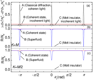
Figure 2: (Color online) Intensity angular distributions for two traveling waves, the pump is transverse to the lattice ($\theta_{0}=0$). (a) Intensity of classical diffraction of coherent light (curve A), isotropic intensity of incoherent light scattering, Eq. (14), for coherent atomic state (line B) and MI state (line C); (b) noise quantity, Eq. (23), for coherent atomic state (constant value 1, line A), SF with all sites illuminated $K=M$ (curve B), and MI (constant value 0, line C); (c) the same as in (b) but for partially illuminated SF with $K=M/2$. $N=M=30$.

For two traveling waves, which can be free-space modes or fixed by ring cavities, the geometrical coefficients (IV.1) are $A_{m}=\exp(im\alpha_{-})$ ($\alpha_{-}=k_{0x}d\sin\theta_{0}-k_{1x}d\sin\theta_{1}$), and Eq. (13e) for the noise quantity is reduced to

$$R=\langle\delta\hat{n}_{a}\delta\hat{n}_{b}\rangle\frac{\sin^{2}{(K\alpha_{-}/2})}{\sin^{2}{(\alpha_{-}/2})}+(\langle\delta\hat{n}^{2}\rangle-\langle\delta\hat{n}_{a}\delta\hat{n}_{b}\rangle)K,$$ (22)

where the first term has the angle dependence of classical diffraction (III), and the angle dependence in the second term in Eq. (13e) is reduced to a constant (isotropic) one, $K$. In the MI and coherent states, where pair correlations $\langle\delta\hat{n}_{a}\delta\hat{n}_{b}\rangle$ are absent, the first term is zero. In the MI state, on-site density fluctuations $\langle\delta\hat{n}^{2}\rangle$ are also zero giving the zero value of the noise quantity (22), while in the coherent state, it is the on-site fluctuations $\langle\delta\hat{n}^{2}\rangle=n$ that give isotropic contribution to $R$. Thus, we have

$$R_{\text{MI}}=0,$$ (23a)

$$R_{\text{Coh}}=nK=N_{K},$$ (23b)

$$R_{\text{SF}_{K}}=-\frac{N}{M^{2}}\frac{\sin^{2}{(K\alpha_{-}/2})}{\sin^{2}{(\alpha_{-}/2})}+\frac{N}{M}K.$$ (23c)

It is important to note, that in the SF state (23c), even in a large optical lattice with $N,M\rightarrow\infty$, very small pair correlations $\langle\delta\hat{n}_{a}\delta\hat{n}_{b}\rangle=-N/M^{2}$ can give a significant angle-dependent contribution to the noise quantity, which occurs near a diffraction maximum ($\alpha_{-}=2\pi l,l=0,1,..$), where the geometrical factor is equal to $K^{2}$, and if the number of the illuminated sites $K$ is of the order of $M$. This demonstrates the importance of nonlocal correlations and invalidity of the coherent-state approximation under those conditions. Outside the diffraction maximum, where the geometrical factor is small, pair correlations do not play any role and the coherent-state approximation works well even for all sites illuminated.

Figure 2 shows several angle dependences of the scattered light in the case of two traveling waves. As an example, in all figures, we will consider atoms at each lattice sites providing $d=\lambda_{0,1}/2$. In Fig. 2(a), the angular distribution of classical diffraction $|\langle D\rangle|^{2}$ (curve A) is shown. In the case of $d=\lambda_{0,1}/2$ and the pump being orthogonal to the lattice ($\theta_{0}=0$), only the zero-order diffraction maxima at $\theta_{1}=0,\pi$ are possible in the classical picture. Corresponding noise quantities $R$ for the coherent (constant lines A) and SF_K (curves B) states are displayed in Figs. 2(b) and 2(c) (in MI, the noise is zero, which is displayed by lines C). According to Eq. (23), the intensity fluctuations are isotropic for the coherent atomic state, while there is suppression of intensity noise under scattering from the SF. The suppression occurs in the regions of diffraction maxima. For all sites illuminated, $K=M$ [cf. Fig. 2(b)], the suppression is total, while for $K=M/2$ it is only partial [cf. Fig. 2(c)]. Outside the maxima, the dependence for SF_K is well approximated by that for the coherent state for any $K$.

It is important to underline, that in a broad range of angles, the number of scattered photons from the SF (or coherent) state is nonzero, even if the expectation value of the electromagnetic field vanishes, which manifests the appearance of nonclassical entanglement between the light and manybody atomic system. Moreover, in contrast to MI state, atoms in SF state scatter photons at angles, where the classical diffraction does not exist.

For example, in a simple configuration considered in Sec. VI where the pump is orthogonal to the lattices ($\theta_{0}=0$), and the scattered light is collected by a cavity along the lattice axis ($\theta_{1}=\pi/2$), the atoms in the MI state scatter no photons as in classical diffraction minimum. In contrast, atoms in the SF_K state scatter the number of photons $a_{1}^{\dagger}a_{1}=|C|^{2}\langle\hat{D}^{*}\hat{D}\rangle=|C|^{2}N_{K}$, proportional to the number of the atoms illuminated [cf. Eq. (23) and Fig. 2(b) at the angle $\theta_{1}=\pi/2$].

For two traveling waves, the expression for $\hat{D}$ (IV.1), in a diffraction maximum where all atoms radiate in phase with each other and $\alpha_{-}=2\pi l$, is reduced to the operator $\hat{N}_{K}$. Thus, the quantity $\langle\hat{D}\rangle=N_{K}=nK$ is the expectation value of the atom number at $K$ sites and proportional to the average atom number at a single site. The intensity of the light scattered into a diffraction maximum is determined by $\langle\hat{D}^{*}\hat{D}\rangle=\langle N_{K}^{2}\rangle$, while noise $R=(\Delta N_{K})^{2}$ gives the atom number variance at $K$ sites. The latter statement corresponds to Figs. 2(b) and 2(c) displaying the total noise suppression in SF_M state, where the total atom number at all sites $K=M$ does not fluctuate, while for $K<M$, $N_{K}$ is a fluctuating quantity and the noise suppression is only partial.

At the angle of a classical diffraction “minimum” (for $K\gg 1$ this is approximately valid for any angle outside narrow regions of maxima), the expectation value of the field amplitude is zero, as well as the first terms in Eqs. (13c), (13d), (13e), and both the intensity $\langle\hat{D}^{*}\hat{D}\rangle$ and noise $R$ are proportional to the quantity $\langle\hat{n}^{2}\rangle-\langle\hat{n}_{a}\hat{n}_{b}\rangle$ giving the difference between local and nonlocal fluctuations. For two traveling waves, the coefficient of proportionality is isotropic and equal to $K$ [cf. Eq. (22)].

For scattering of incoherent light (14), the intensity is proportional to the local quantity $\langle\hat{n}^{2}\rangle$ and is shown in Fig. 2(a) for MI (curve C) and coherent, almost the same as in SF, (curve B) states. This quantity can be also obtained under coherent scattering of two traveling waves, if one tunes the angles such that the geometrical factor of the first term in Eq. (22) is equal to $K$. Practically, this variant is easy to achieve only for a diffraction pattern with diffraction maxima, which are not too narrow.

Hence, in an optical experiment, both global statistical quantities related to $K\leq M$ sites, local quantities reflecting statistics at a single site, and pair correlations can be obtained. It is important, that local statistics can be determined by global measurements, i.e., an optical access to a single site is not necessary.

Therefore, light scattering gives a possibility to distinguish different quantum states of ultracold atoms. As demonstrated by Eq. (23) and Fig. 2, MI and SF_M states are distinguishable in diffraction “minima” and in incoherent light, while they are indistinguishable (for traveling waves) in maxima, because the total atom number contributing to the maximum does not fluctuate. The SF_M and coherent states can be distinguished in diffraction maxima only. The MI and coherent states can be distinguished in any angle of the scattering pattern.

Measurements of the noise quantity discussed or, alternatively, related quantities for quadratures (16) or photon number variance (IV.3), give the values, which are different in orders of the emitter number $N_{K}$ for different quantum states. Nevertheless, for large $N_{K}$, there could be practical problems in the subtraction of large values in a diffraction maximum to get the noise contribution. In some papers, a similar problem even led to a conclusion about state indistinguishability by intensity measurements in BEC Idziaszek et al. (2000); Cirac et al. (1994a, b) and, hence, to a necessity to measure photon statistics. A rather involved method to suppress the strong classical part of scattering using a dark-state resonance in BEC was proposed in Ref. Müstecaplioglu and You (2001). In contrast to homogeneous ensembles, in optical lattices, this problem has a natural solution: measurements outside diffraction maxima are free of the strong classical-like part and thus directly reflect density fluctuations.

VII.2 Physical interpretation and role of the entanglement between light and matter

The classical analogy of the difference in light scattering from different atomic states consists in various density fluctuations in different states. In particular, classical density fluctuations would also lead to impossibility of obtaining a perfect diffraction minimum, where contributions from all sites should precisely cancel each other.

Scattering at diffraction maxima can be treated as superradiant one, since the intensity of the scattered light is proportional to the number of phase-synchronized emitters squared $N_{K}^{2}$. In diffraction minima, destructive interference leads to the total (subradiant) suppression of coherent radiation for MI state; whereas for SF_K state, the intensity is nonzero and proportional to the number of emitters $N_{K}$, which is analogous to the emission of independent (non-phase-synchronized) atoms.

Nevertheless, the quantum treatment gives a deeper insight into the problem.

The expression for the SF state in Table 1 can be rewritten in the following from:

$$|\Psi_{\text{SF}}\rangle=\frac{1}{(\sqrt{M})^{N}}\sum_{q_{i}}\sqrt{\frac{N!}{q_{1}!q_{2}!...q_{M}!}}|q_{1},q_{2},..q_{M}\rangle,$$

where the sum is taken over all $q_{i}$ such that $\sum_{i}^{M}q_{i}=N$. It shows that the SF state is a quantum superposition of all possible multisite Fock states corresponding to all possible distributions of $N$ atoms at $M$ lattice sites. Under the light–matter interaction, the Fock states corresponding to different atomic distributions become entangled to scattered light of different phases and amplitudes OptCom ; Andras .

For example, in a simple case of two atoms at two sites, $|\Psi_{\text{SF}}\rangle=1/2|2,0\rangle+1/\sqrt{2}|1,1\rangle+1/2|0,2\rangle$. In the example configuration of Sec. VI, where the orthogonal pump illuminates lattice sites separated by $\lambda/2$ (diffraction minimum), the wave function of the whole light-matter system reads

$$|\Psi_{\text{matter-light}}\rangle=1/2|2,0\rangle|\gamma\rangle+1/\sqrt{2}|1,1\rangle|0\rangle$$

$$+1/2|0,2\rangle|-\gamma\rangle.$$

Here, if we assume that the distribution $|2,0\rangle$ is entangled to the coherent state of light $|\gamma\rangle$, the distribution $|0,2\rangle$ will be entangled to the similar light state with the opposite phase $|-\gamma\rangle$, and the distribution $|1,1\rangle$ will be entangled to the vacuum field $|0\rangle$, because the fields emitted by two atoms cancel each other.

In contrast to the classical case, light fields entangled to various atomic distributions do not interfere with each other, which is due to the orthogonality of the Fock states, providing a sort of which-path information. This leads to a difference from the classical (or MI with the only Fock state $|1,1\rangle$) case and nonzero expectation value of the photon number even in the diffraction minimum ($|\gamma|^{2}/2$ in the above example). The absence of interference gives also an insight into the similarity of scattering from the SF state to the scattering from independent (non-phase-synchronized) atoms, where interference is also absent.

We would like to mention that light measurements considered here correspond to the QND measurements Brune of atomic variables observing light. Considering the Hamiltonian (II) with neglected tunneling, it is straightforward to show that for the “probe observable” (i.e. measured light $a_{1}^{\dagger}a_{1}$) and “signal observable” $\hat{D}$ (10b), all four conditions of the QND scheme summarized in Ref. Brune are fulfilled. Thus, observing light one can determine various atomic functions corresponding to the geometry-dependent operator $\hat{D}$ (10b) in a QND way. For example, the total atom number or atom number at some lattice region can be nondestructively measured in a diffraction maximum, while the difference between atom numbers at odd and even sites can be nondestructively determined in a diffraction minimum.

VII.3 Standing waves

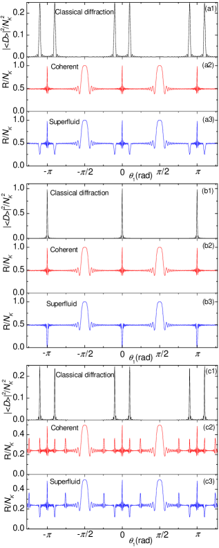
Figure 3: (Color online) Intensity angular distributions for scattering into a standing-wave cavity. (a) Traveling-wave pump at $\theta_{0}=0.1\pi$; (b) traveling or standing-wave pump at $\theta_{0}=0$; (c) standing-wave pump at $\theta_{0}=0.1\pi$. Intensities of classical diffraction are shown in Figs. (a1), (b1), and (c1); noise quantities for coherent state are shown in Figs. (a2), (b2), and (c2) and for SF in Figs. (a3), (b3), and (c3). $N=M=K=30$.

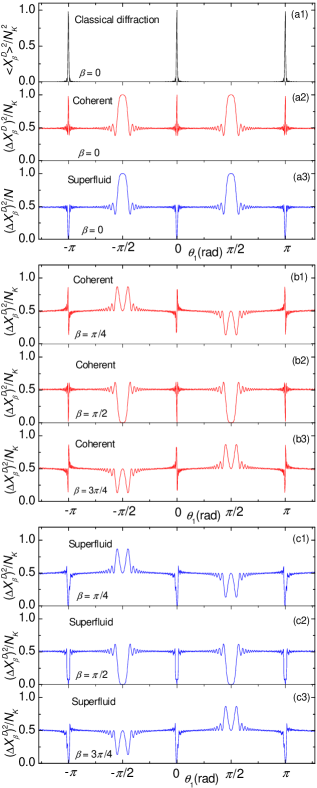
Figure 4: (Color online) Quadrature angular distributions for two traveling waves. (a) Quadrature for classical diffraction (a1), quadrature variance for coherent (a2) and SF (a3) states, pump-homodyne phase difference $\beta=0$; (b) quadrature variance for coherent state for $\beta=\pi/4$ (b1), $\beta=\pi/2$ (b2), $\beta=3\pi/4$ (b3); (c) quadrature variance for SF for $\beta=\pi/4$ (c1), $\beta=\pi/2$ (c2), $\beta=3\pi/4$ (c3). $\theta_{0}=0$, $N=M=K=30$.

If at least one of the modes is a standing wave, the angle dependence of the noise becomes richer. In an experiment, this configuration corresponds to a case where the scattered light is collected by a standing-wave cavity, whose axis can by tuned with respect to the lattice axis Maschler and Ritsch (2005). Except for the appearance of new classical diffraction maxima represented by the first terms in Eqs. (13c), (13d), (13e), which depend on the phase parameters $\alpha_{\pm}=k_{0x}d\sin\theta_{0}\pm k_{1x}d\sin\theta_{1}$, the angle dependence of the second term is also not an isotropic one, as it was for two traveling waves. This second, “noise,” term includes a sum of the geometrical coefficients squared, which is equivalent to the effective doubling of the lattice period (or doubling of the light frequency) and leads to the appearance of new spatial harmonics in the light angular distribution. Such period doubling leads to the appearance of the peaks in the noise distribution at the angles, where classical diffraction does not exists.

In Fig. 3(a), angular distributions of the scattered light are shown for a traveling-wave pump, which is almost orthogonal to a lattice ($\theta_{0}=0.1\pi$), while the probe is a standing wave. Classical diffraction pattern [cf. Fig. 3(a1)] is determined by $|A|^{2}$ through the parameters $\alpha_{\pm}$ and shows zero-order diffraction maxima in transmission ($\theta_{1}=\theta_{0}$ and its counterpart due to the presence of the standing-wave cavity at $\theta_{1}=\pi+\theta_{0}$) and reflection ($\theta_{1}=\pi-\theta_{0}$ and the counterpart at $-\theta_{0}$). The intensity noise for atoms in the coherent state [cf. Fig. 3(a2)] is determined by $\sum_{i=1}^{K}{|A_{i}|^{2}}$ through another parameter $2\alpha_{1}=2k_{1x}d\sin\theta_{1}$ and has different characteristic features at $\theta_{1}=0,\pi$, and $\pm\pi/2$. It is the latter feature that corresponds to the effective frequency doubling and appears at an angle, where classical diffraction has a minimum. In the case of SF_M state [cf. Fig. 3(a3)], pair correlations in Eqs. (13d) and (13e) are nonzero, hence, both geometrical factors contribute to the noise distribution, which has the features at angles characteristic to both classical scattering and the light noise of the coherent-state case. Outside the characteristic features, the noise distribution is isotropic and takes a nonzero value similar to the case of two traveling waves [cf. Fig. 2]. Figure 3(b) shows a simpler situation, where the pump is precisely orthogonal to the lattices ($\theta_{0}=0$).

In Fig. 3(c), a situation similar to Fig. 3(a) is shown for the case where both the pump and probe are standing waves. While classical diffraction still depends on the parameters $\alpha_{\pm}$, the factor $\sum_{i=1}^{K}{|A_{i}|^{2}}$ determining the intensity noise depends on four parameters $2\alpha_{0,1}=2k_{0,1x}d\sin\theta_{0,1}$ and $2\alpha_{\pm}$. Thus, in the light noise from a lattice in the coherent and SF states, the features are placed at the positions of classical zero-order diffraction maxima and the angles, which would correspond to the classical scattering from a lattice with a doubled period $d=\lambda$, where the appearance of first-order diffraction maxima is possible. Similar to Fig. 3(a), features at $\theta_{1}=0,\pi$, and $\pi/2$ also exist. In the case $\theta_{0}=0$, the angular distribution for two standing waves is identical to that of one standing wave shown in Fig. 3(b).

In the SF_M state, there are two types of diffraction maxima. In the first one, the noise can be completely suppressed due to the total atom number conservation, similarly to the case of traveling waves. This occurs, if the condition of the maximum is fulfilled for both of two traveling waves forming a single standing wave [cf. Fig. 3(b)]. In the second type, even for $K=M$, only partial noise suppression is possible, since only one of the traveling waves is in a maximum, while another one, being in a minimum, produces the noise [cf. Figs. 3(a) and 3(c)]. In contrast to two traveling modes, in the second type of maxima, one can distinguish between SF_M and MI states, since MI produces no noise in any direction.

VII.4 Quadratures and photon statistics

An analysis of the angular distribution of the quadrature variance $(\Delta X_{\beta}^{D})^{2}$ (16b) shows, that even for two traveling waves, new peaks due to effective period doubling appear [see Fig. 4(a)]. Additionally, the amplitude of noise features can be varied by the phase difference between the pump and homodyne beams $\beta$, which is shown in Figs. 4(b) for the coherent and in Fig. 4(c) SF_M states. In the coherent state, all peaks are very sensitive to $\beta$. In the SF_M state, the noise suppression at diffraction maxima is insensitive to variations of $\beta$, whereas other peaks are $\beta$-dependent. The relation of $(\Delta X_{\beta}^{D})^{2}$ to the quadrature variance of the light field is given by Eq. (15c).

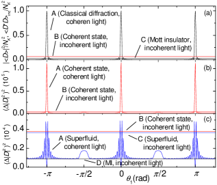
Figure 5: (Color online) Angular distributions of photon-number variances for two traveling waves. (a) Intensity of classical diffraction (curve A), isotropic intensity of incoherent light scattering, Eq. (14), for coherent atomic state (line B) and MI state (line C); (b) normal ordered photon-number variance for coherent atomic state under scattering of coherent, Eq. (VII.4) (curve A), and incoherent (line B) light; (c) normal ordered photon-number variance for SF state under scattering of coherent, Eq. (VII.4) (curve A), and incoherent (line C) light, variance for coherent (line B) and MI (curve D) states under scattering of incoherent light. Normal ordered photon-number variance for MI state under scattering of coherent light is zero for all angles. $\theta_{0}=0$, $N=M=K=30$.

The angle dependence of the variance $(\Delta|D|^{2})^{2}=\langle\hat{D}^{*2}\hat{D}^{2}\rangle-\langle\hat{D}^{*}\hat{D}\rangle^{2}$, which is proportional to the normal ordered photon-number variance and determines the light statistics (IV.3), also shows anisotropic features due to frequency doubling even for two traveling waves (Fig. 5). In this case, Eq. (IV.3) is reduced to

$$\langle\hat{D}^{*2}\hat{D}^{2}\rangle=\left(\frac{\sin(K\alpha_{-}/2)}{\sin(\alpha_{-}/2)}\right)^{4}\langle n_{a}n_{b}n_{c}n_{d}\rangle+2\left(\frac{\sin(K\alpha_{-}/2)}{\sin(\alpha_{-}/2)}\right)^{3}\frac{\cos(K\alpha_{-}/2)}{\cos(\alpha_{-}/2)}(\langle n_{a}^{2}n_{b}n_{c}\rangle-\langle n_{a}n_{b}n_{c}n_{d}\rangle)$$

$$-4\left(\frac{\sin(K\alpha_{-}/2)}{\sin(\alpha_{-}/2)}\right)^{2}[(K-2)\langle n_{a}n_{b}n_{c}n_{d}\rangle-(K-3)\langle n_{a}^{2}n_{b}n_{c}\rangle-\langle n_{a}^{3}n_{b}\rangle]$$

$$+\left(\frac{\sin K\alpha_{-}}{\sin\alpha_{-}}\right)^{2}(\langle n_{a}n_{b}n_{c}n_{d}\rangle-2\langle n_{a}^{2}n_{b}n_{c}\rangle+\langle n_{a}^{2}n_{b}^{2}\rangle)+2K^{2}(\langle n_{a}n_{b}n_{c}n_{d}\rangle-2\langle n_{a}^{2}n_{b}n_{c}\rangle+\langle n_{a}^{2}n_{b}^{2}\rangle)$$

$$+K(-6\langle n_{a}n_{b}n_{c}n_{d}\rangle+12\langle n_{a}^{2}n_{b}n_{c}\rangle-4\langle n_{a}^{3}n_{b}\rangle-3\langle n_{a}^{2}n_{b}^{2}\rangle+\langle n^{4}\rangle),$$ (24)

where the first four terms has features at angles typical to classical diffraction, the fourth term is also responsible for the doubled-frequency feature, and the last two terms contribute to the isotropic component.

For the coherent state, the light scattered into a diffraction maximum displays a very strong noise (equal to $4N_{K}^{3}+6N_{K}^{2}+N_{k}$ because $\langle\hat{D}^{*2}\hat{D}^{2}\rangle=N_{K}^{4}+6N_{K}^{3}+7N_{K}^{2}+N_{k}$ and $\langle\hat{D}^{*}\hat{D}\rangle=N_{K}^{2}+N_{K}$), which is much stronger than the isotropic component ($N_{K}^{2}$ in highest order of $N_{K}$) and the features at $\theta_{1}=\pm\pi/2$ ($2N_{K}^{2}$ in highest order of $N_{K}$) [Fig. 5(b)]. In SF_M state, the noise at maxima can be suppressed, while at other angles, in highest order of $N_{K}$, it is equal to that of the coherent state [Fig.5(c)]. In MI state, the variance $(\Delta|D|^{2})^{2}$ is zero for all angles. Conclusions about state distinguishing by measuring light statistics are very similar to those drown from the intensity and amplitude measurements, which have been discussed in Sec. VIIA, including scattering of incoherent light (see Fig. 5 and the discussion of Fig. 2).

In experiments, the nontrivial angle dependence of the noise can help in the separation of the light noise reflecting atom statistics from technical imperfections.

VIII Conclusions

We studied off-resonant collective light scattering from ultracold atoms trapped in an optical lattice. Measuring the light field allows to characterize the quantum state of atoms in a nondestructive way and in particular distinguish between different atomic states. The scattered light differs in intensity, quadrature variances, and photon statistics. A measurement of the intensity angular distribution provides information about atom number fluctuations in a finite lattice region, local quantum statistics at single sites, and pair correlations. Note that even local statistics can be determined by global measurements without an optical access to particular sites. Alternatively to angle-resolved measurements, variations of the mode wavelengths with respect to the wavelength of a trapping beam can be considered.

Light scattering as a diagnostic tool has particular advantages for optical lattices in contrast to scattering from a homogeneous BEC. Here one has a natural way to suppress the strong classical scattering background by looking at the directions of diffraction minima. In these directions the expectation value of the field amplitude vanishes while the intensity (photon number) is nonzero and directly reflects quantum fluctuations. Furthermore, in an optical lattice, the signal is sensitive not only to the periodic density distribution, but also to the periodic density fluctuations, giving an access to even very small nonlocal pair correlations. These can be obtained by measuring light at diffraction maxima.

As the most striking example, we considered light scattering from a 1D lattice in a transversally pumped optical cavity as in a setup involving collective cavity cooling Domokos and Ritsch (2002); Black et al. (2005); Elsässer et al. (2004); Slama et al. (2005). The number of photons scattered into the cavity is zero for the Mott insulator phase but proportional to the atom number in the superfluid phase. Both states have almost the same average density but different quantum uncertainties. So the superfluid state is a quantum superposition of different Fock states corresponding to all possible distributions of $N$ atoms at $M$ sites. Under illumination by a coherent light, various Fock states become entangled to scattered light states with different amplitudes and phases. In contrast to classical scattering, where the atoms are described by c-number center-of-mass positions Eichmann et al. (1993), for a quantum description of the atomic motion the light field amplitudes corresponding to different atomic distributions do not interfere. This is due to the orthogonality of Fock states forming the superfluid providing a sort of which way information.

In the example configuration, the cavity-field amplitude is determined by the atom number operators $\hat{n}_{i}=b^{\dagger}_{i}b_{i}$. Hence, the expectation value of the field amplitude is sensitive to the average density only. In contrast, the intracavity photon number reflects the second moments of atom number operators (e.g. density-density correlations), while photon statistics reflects the forth moments.

Let’s emphasize that other physical systems are possible, where the light amplitude depends on the matter-field amplitudes $b_{i}$, while the intensity is sensitive to density operators $\hat{n}_{i}$. The latter situation is typical to configurations, where two or more atomic subsystems exist and can interact with each other, in particular, through light fields. The examples are matter-wave superradiance and amplification, where two or more momentum states of cold atoms were observed Inouye et al. (1999); Moore et al. (1999); Pu et al. (2003); Trifonov (2005), and interaction between two BECs with different internal Zeng et al. (1995); Ruostekoski and Walls (1997); Search and Berman (2001); Search (2001) or motional Ruostekoski et al. (1998) atomic states. In the framework of our paper, matter-field amplitudes $b_{i}$ can also contribute to light amplitudes $a_{l}$, if the tunneling between lattice sites is important, which we have considered in the general model in Sec. II. In the rest of the paper, the lattice was assumed deep leading to negligible tunneling.

In general, a variety of optical effects can be sensitive to a quantum state of an ultracold matter, if the density operators enter measurable quantities nonlinearly, such that the expectation value of those quantities cannot be simply expressed through expectation values of density operators. For instance, the $\chi^{(3)}$ nonlinearity Hiroshima and Yamamoto (1996) and refractive index of a gas, where nonlocal field effects are important Morice et al. (1995), were shown to depend on atom statistics. In this paper, we focused on such nonlinear quantities as intensity, quadrature variances, and photon statistics of scattered light meystre . Phase-sensitive and spectral characteristics mentioned in Sec. IV.D reflect the dependence of the dispersion of a medium on the quantum state of matter WeArxiv07 ; ICAP . Moreover, such dispersion effects (e.g. cavity-mode shift) will reflect atom statistics not only in light intensity, but even in light amplitudes $\langle a_{l}\rangle$.

So far we have neglected the dynamic back action of scattered field on atoms. This can be well justified in a deep lattice where the momentum transfer is by far not enough to change the atomic vibrational state as long as not too many photons are scattered. Even without energy transfer the information one gets from the light will induce measurement back-action. This should have intriguing consequences for multiple consecutive measurements on the light scattered from optical lattices.