$\stackrel{{\scriptstyle\rm\textstyle DSF-57/97}}{{\rm\textstyle quant-ph/9802030}}$
Time–Dependent Invariants and Green Functions in the Probability Representation of Quantum Mechanics

Abstract

In the probability representation of quantum mechanics, quantum states are represented by a classical probability distribution, the marginal distribution function (MDF), whose time dependence is governed by a classical evolution equation. We find and explicitly solve, for a wide class of Hamiltonians, new equations for the Green’s function of such an equation, the so–called classical propagator. We elucidate the connection of the classical propagator to the quantum propagator for the density matrix and to the Green’s function of the Schrödinger equation. Within the new description of quantum mechanics we give a definition of coherence solely in terms of properties of the MDF and we test the new definition recovering well known results. As an application, the forced parametric oscillator is considered . Its classical and quantum propagator are found, together with the MDF for coherent and Fock states.

Introduction

Quantum states are usually described in terms of wave functions [1] (for pure states) or by means of the density matrix [2], [3] (for mixed states). Nonetheless, since the beginning of quantum mechanics there have been attempts of understanding the notion of quantum states in terms of a classical approach [4, 5]. Due to the Heisenberg principle, it is not possible to introduce a joint distribution function for both coordinates and momenta, while these joint probability distributions are the main tool to describe physical states in classical statistical mechanics. It is such kind of problems which has brought to the introduction of the so called quasi–probability distribution functions, such as the Wigner function [6], the Husimi function [7] and the Glauber–Sudarshan function [8], [9], later on unified into a one–parametric family [10]. Despite their wide use in quantum theory and their fundamental rôle in clarifying the link among classical and quantum aspects, these quasi–probability distributions cannot play the rôle of classical distributions since, either they allow for negative values (like the Wigner function) or they do not describe distributions of measurable variables. A formulation of quantum mechanics which is very similar to the classical stochastic approach has been presented by Moyal [11]. But, the evolution equation suggested by Moyal was an equation for a quasi–probability distribution function (the Wigner function) and not for the probability.

In [12, 13] it was recently suggested to consider quantum dynamics as a classical stochastic process described namely by a probability distribution: the so called marginal distribution function (which was discussed in a general context in [10]), associated to the position coordinate, $X$, taking values in an ensemble of reference frames in the phase space. Such a classical probability distribution is shown to completely describe quantum states [14, 15]. The approach of [12]-[15] was developed both for quadrature observables [16]-[19] and for spin [20].

Within this approach the notion of “measuring a quantum state” provides the usual “optical tomography approach” [21, 22, 23] and its extension called the “symplectic tomography” formalism [14, 15]. Both allow for an explicit link between the MDF and the Wigner function or the density matrix, in other representations. In this way, starting from the evolution equation for the density matrix, an evolution equation of the Fokker-Plank type for the marginal distribution function is obtained [12, 13]. Such an equation allows for an independent definition of the marginal distribution function. Thus it may be assumed as the starting point for an alternative but equivalent formulation of quantum mechanics in what we call the probability representation, or classical-like description of quantum mechanics. In such a scheme, it plays the same rôle that the Schrödinger equation plays in the usual approach to quantum mechanics. Since the MDF may be interpreted as a classical probability distribution, the Green’s function connected to its evolution equation is called the classical propagator. In [16] the classical propagator for a wide class of Hamiltonians and its relation to the quantum propagator for the density matrix are found. This establishes an important bridge among the probability representation of quantum mechanics and other formulations such as the path integral approach.

The present work deals with two different problems. On one side we extend the emerging new description of quantum mechanics; on the other, we verify the formalism by applying it to a concrete, non–trivial case of physical interest, which is the forced parametric oscillator. A short report on the new results which we are going to present is already contained in [24]. From the point of view of the general formalism, we find new equations which connect the classical propagator of a quantum system to its integrals of motion. Also, we give a new definition of coherence, solely in terms of properties of the MDF, which relates the coherent marginal distribution function to invariants of the quantum system. In this regard let us note that the general approach to time-dependent invariants in quantum mechanics and their relation to the wave function were elucidated by Lewis and Riesenfeld in [25], while the connection among integrals of the motion and the quantum propagator was found in [26, 27]. In [28] the relation of time-dependent invariants to the Schwinger action principle was established, and in [29] the relation with the Nöther theorem was discussed.

Let us come to the forced parametric oscillator. This is a phenomenologically interesting model as it yields a good description of physical systems, like for example ions in a Paul trap. For such a system the symplectic tomography was already discussed in [18] while the endoscopy scheme for measuring states was suggested in [30]. The trapped ion may be in different nonclassical states like nonlinear coherent states [31]. A general analysis of such states may be found in [32]. Here we try a complete description of the model in the framework of the new scheme.

In section 1 we review the formulation of quantum mechanics in the probability representation. We introduce the marginal distribution function, together with its evolution equation. Then, we discuss the relation among the classical and quantum propagators and we specialize to the case of quadratic Hamiltonians. In section 2 we find two new equations for the classical propagator which is shown to be eigenfunction of a certain time-dependent invariant. We solve these equations for quadratic Hamiltonians and obtain the classical propagator as a function of time-dependent invariants of the system. This is an important step towards the characterization of the quantum system, as it yields both the quantum propagator for the density matrix (which we use to test the scheme by comparing our results to well known results achieved by usual methods) and the time-dependence of the MDF, once it is known at $t=0$. In section 3 we give a characterization of coherence directly in terms of the MDF, and we test the new approach by explicitly finding the coherent marginal distribution for the forced parametric oscillator both in the new framework and by means of more conventional methods. Finally we find the MDF for Fock states and we show a few significant plots.

I The Probability Representation of Quantum Mechanics

In ref. [14] an operator $\hat{X}$ is discussed as a generic linear combination of position and momentum operators

$$\hat{X}=\mu\hat{q}+\nu\hat{p}$$ (I.1)

where $\mu,~{}\nu,$ are real parameters and $\hat{X}$ is hermitian, hence observable. The physical meaning of $\mu,\nu$ is that they describe an ensemble of rotated and scaled reference frames, in classical phase space, in which the position $X$ may be measured. In the above mentioned paper it is shown that the quantum state of a system is completely determined if the classical probability distribution, $w(X,\mu,\nu)$, for the variable $X$, is given in an ensemble of reference frames in the classical phase space. Such a function, also known as the marginal distribution function, belongs to a broad class of distributions which are determined as the Fourier transform of a characteristic function [10]. For the particular case of the variable (I.1), considered in [12]-[15], the scheme of [10] gives

$$w(X,\mu,\nu)={1\over 2\pi}\int dke^{-ikX}<e^{ik\hat{X}}>~{},$$ (I.2)

where $<\hat{A}>=\mbox{\rm Tr}(\hat{\rho}\hat{A})$, and $\hat{\rho}$ is the density operator. In [10] it was shown that, whenever $\hat{X}$ is an observable, $w(X,\mu,\nu)$ is indeed a probability distribution, as it is positive definite and satisfies the normalization condition

$$\int w(X,\mu,\nu)dX=1~{}.$$ (I.3)

The definition of the MDF allows us to express it in terms of the density matrix

$$w(X,\mu,\nu)={1\over 2\pi\nu}\int\rho(Z,Z^{\prime})\exp\left[-i{Z-Z^{\prime}\over\nu}\left(X-\mu{Z+Z^{\prime}\over 2}\right)\right]dZdZ^{\prime}~{}.$$ (I.4)

Recalling the relation among the Wigner function and the density matrix, (I.4) may be rewritten as a relation among $w$ and the Wigner function ,

$$w(X,\mu,\nu)=\int\exp[-ik(X-\mu q+\nu p)]W(q,p){dk~{}dp~{}dq\over(2\pi)^{2}}~{}.$$ (I.5)

Although the general class of distribution functions of the kind (I.2) was introduced, as a function of the density matrix, already by Cahill and Glauber in [10], they didn’t analyze the possibility of a new approach to quantum mechanics, in terms of such distribution functions, mainly because the invertibility of (I.4) was not investigated. An important step in this direction is represented by [31] where Vogel and Risken have shown that for a particular choice of the parameters $\mu$ and $\nu$ (the homodyne quadrature) the marginal distribution determines completely the Wigner function via Radon transform, namely they prove that (I.5) may be inverted for the Wigner function. In the same spirit, it was shown in [12, 13] that the relation among $w$ and the density matrix can be inverted for $\rho$ yielding

$$\rho(X,X^{\prime})={1\over 2\pi}\int w(Y,\mu,X-X^{\prime})\exp\left[i\left(Y-\mu{X+X^{\prime}\over 2}\right)\right]d\mu dY~{}.$$ (I.6)

and, because of such a relation, the marginal distribution function satisfies an evolution equation

$$\partial_{t}w+\hat{O}w=0~{},$$ (I.7)

where $\hat{O}$ is a finite or infinite operator polynomial in $\hat{q}$, $\hat{p}$ (also depending on $\mu,~{}\nu$), determined by the Hamiltonian. Hence, we make our previous statements more precise, by saying that the MDF (the classical probability associated to the random variable $X$) contains the same information on a quantum system as the density matrix. The MDF may be defined through (I.7) independently from the density matrix, hence it represents the starting point for an alternative (but equivalent) approach to quantum mechanics, while (I.7) may be thought of as the analogue of the Schrödinger equation. Eq. (I.7) can be formally integrated to give

$$w(X,\mu,\nu,t)=\int\Pi(X,\mu,\nu,0,X^{\prime},\mu^{\prime},\nu^{\prime},t)w(X^{\prime},\mu^{\prime},\nu^{\prime},0)dX^{\prime}d\mu^{\prime}d\nu^{\prime}~{},$$ (I.8)

where $\Pi(X,\mu,\nu,0,X^{\prime},\mu^{\prime},\nu^{\prime},t)$ is the Green’s function for the evolution equation (I.7). This is what we call the classical propagator. It can be interpreted as the classical transition probability density from an initial position $X^{\prime}$ in the ensemble of reference frames of the classical phase space, to the position $X$ [13].

Let us now elucidate the connection of the classical propagator with the quantum propagator (Green function) for the density matrix $\rho(X,X^{\prime},t)$. Details may be found in [16, 19]. For a pure state with wave function $\Psi(X,t)$, we have

$$\rho(X,X^{\prime},t)=\Psi(X,t)\Psi^{*}(X^{\prime},t).$$ (I.9)

Since the wave function at time $t$ is connected to the one at initial time by the Green’s function of the Schrödinger equation $G(X,X^{\prime},t)$

$$\Psi(X,t)=\int\Psi(X^{\prime},0)G(X,X^{\prime},t)dX^{\prime}$$ (I.10)

we have for the density matrix

$$\rho(X,X^{\prime},t)=\int K(X,X^{\prime},Y,Y^{\prime},t)\rho(Y,Y^{\prime},0)dYdY^{\prime}$$ (I.11)

with

$$K(X,X^{\prime},Y,Y^{\prime},t)=G(X,Y,t)G^{*}(X^{\prime},Y^{\prime},t).$$ (I.12)

The function $K(X,X^{\prime},Y,Y^{\prime},t)$ is what is called the quantum propagator for the density matrix. Using the relation between the density matrix and the MDF (I.6) we finally find

$$K(X,X^{\prime},Z,Z^{\prime},t) = {1\over(2\pi)^{2}}$$ (I.13)

$$\times \int{1\over\nu^{\prime}}\exp\left\{i\left(Y-\mu{X+X^{\prime}\over 2}\right)-i{Z-Z^{\prime}\over\nu^{\prime}}Y^{\prime}+i{Z^{2}+Z^{\prime 2}\over 2\nu^{\prime}}\mu^{\prime}\right\}$$ (I.14)

$$\times \Pi(Y,\mu,X-X^{\prime},0,Y^{\prime},\mu^{\prime},\nu^{\prime},t)d\mu d\mu^{\prime}dYdY^{\prime}d\nu^{\prime}~{}.$$ (I.15)

Then, once the classical propagator is known, the quantum propagator for the density matrix can be found. In the next sections, after finding the classical propagator, we will give an explicit example of this kind of calculation, for the driven parametric oscillator. We will also compare our results to analogous calculations obtained with the method of path integrals [33].

II The classical propagator

In this section we address the problem of finding the classical propagator, in the framework of the time-dependent invariants method. We consider Hamiltonians of the form

$$\hat{H}=\frac{\hat{p}^{2}}{2}+V(\hat{q})$$ (II.1)

where $V(q)$ is a generic potential energy. In this case the evolution equation for the MDF, Eq. (I.7), takes the form [12, 13, 16]

$$\dot{w}-\mu{\partial\over\partial\nu}w-i\left[V\left(\frac{-1}{\partial/\partial x}\frac{\partial}{\partial\mu}-i\frac{\nu}{2}\frac{\partial}{\partial x}\right)-V\left(\frac{-1}{\partial/\partial x}\frac{\partial}{\partial\mu}+i\frac{\nu}{2}\frac{\partial}{\partial x}\right)\right]w=0.$$ (II.2)

Restoring the proper units, the Planck constant $\hbar$ will appear in Eq. (II.2) so that the equation, even if classical-like, gives a quantum description of the system evolution, so replacing the Schrödinger equation in our scheme. It can be shown [19] that in classical statistical mechanics the distribution $w(X,\mu,\nu)$ may be also introduced and the classical Boltzmann equation can be rewritten for this distribution. Then the classical limit of (II.2) is the Boltzmann equation. The classical propagator obeys an evolution equation which follows from (II.2)

$$\frac{\partial\Pi}{\partial t_{2}}-\mu{\partial\over\partial\nu}\Pi-i\left[V\left(\frac{-1}{\partial/\partial x}\frac{\partial}{\partial\mu}-i\frac{\nu}{2}\frac{\partial}{\partial x}\right)-V\left(\frac{-1}{\partial/\partial x}\frac{\partial}{\partial\mu}+i\frac{\nu}{2}\frac{\partial}{\partial x}\right)\right]\Pi$$ (II.3)

$$=\delta(t_{2}-t_{1})\delta(X^{\prime}-X)\delta(\mu^{\prime}-\mu)\delta(\nu^{\prime}-\nu),$$ (II.4)

with initial condition

$$\Pi(X,\mu,\nu,0,X^{\prime},\mu^{\prime},\nu^{\prime},0)=\delta(X^{\prime}-X)\delta(\mu^{\prime}-\mu)\delta(\nu^{\prime}-\nu)~{}.$$ (II.5)

To be definite, let us consider the Hamiltonian describing the forced parametric oscillator. This is of the form described by (II.1), and it includes many other quadratic Hamiltonians as limiting cases. The potential, $V(q)$, is given by

$$V(q)={\omega^{2}(t)\over 2}q^{2}-f(t)q,$$ (II.6)

that is

$$H={p^{2}\over 2}+{\omega^{2}(t)\over 2}q^{2}-f(t)q~{}.$$ (II.7)

We leave $\omega$ free to be real or imaginary, to allow the description of repulsive oscillators as well. The evolution equation for the marginal distribution $w$, is obtained by the general expression (II.2), replacing the potential by (II.6). We have

$$\dot{w}-\mu{\partial\over\partial\nu}w+\left(\omega^{2}(t)\nu{\partial\over\partial\mu}+f(t)\nu{\partial\over\partial X}\right)w=0~{}.$$ (II.8)

The equation for the propagator may be obtained analogously.

The solution to (II.4) was previously argued to be expressible in terms of the integrals of the motion of the system [19]. We show here a derivation of this result, which is essentially an extension of previous techniques [25, 26, 27, 29, 28]. In the mentioned papers the time-dependent invariants of a given system were shown to be in connection with the wave function and with the Green function of the Schrödinger equation. The integrals of the motion, $I(t)$ are defined by the equation

$${\partial\over\partial t}I(t)+i[H,I(t)]=0~{},$$ (II.9)

where $H$ is the Hamiltonian of the system. We may think of time-dependent invariants as the evolution in time of the initial coordinates and momenta, $q$ and $p$. Then we express them as

$$I(t)=\Lambda(t)Q+\Delta(t)$$ (II.10)

with $Q=(p,q)$ and $\Lambda,\Delta$ to be determined. For the oscillator any integral of the motion may be expressed as a function of the two operators $A(t)=UaU^{-1}$ and $A^{{\dagger}}(t)=Ua^{\dagger}U^{-1}$, where $U$ is the evolution operator obtained by the Schrödinger equation. Of course, they are integrals of the motion in their turn. We have

$$A(t) = {i\over\sqrt{2}}(\epsilon(t)p-\dot{\epsilon}(t)q)+\beta(t)$$ (II.11)

$$A^{{\dagger}}(t) = -{i\over\sqrt{2}}(\epsilon^{*}(t)p-\dot{\epsilon}^{*}(t)q)+\beta^{*}(t),$$ (II.12)

with $\epsilon$ satisfying

$$\ddot{\epsilon}+\omega^{2}(t)\epsilon = 0$$ (II.13)

$$\dot{\epsilon}\epsilon^{*}-\dot{\epsilon}^{*}\epsilon = 2i$$ (II.14)

and initial conditions $\epsilon(0)=1$, $\dot{\epsilon}(0)=i$. It can be checked that

$$[A,A^{{\dagger}}]=1$$ (II.15)

The function $\beta(t)$ is determined by consistency with (II.9) to be

$$\beta(t)=-{i\over\sqrt{2}}\int_{0}^{t}dt^{\prime}~{}\epsilon(t^{\prime})f(t^{\prime})~{}.$$ (II.16)

The integral of the motion

$$I(t)=\pmatrix{I_{p}\cr I_{q}}=\pmatrix{\Lambda_{11}&\Lambda_{12}\cr\Lambda_{21}&\Lambda_{22}}\pmatrix{p\cr q}+\pmatrix{\Delta_{1}\cr\Delta_{2}}$$ (II.17)

can be given in terms of $A$ and $A^{{\dagger}}$ as

$$I_{p} = {A-A^{{\dagger}}\over\sqrt{2}i}$$ (II.18)

$$I_{q} = {A+A^{{\dagger}}\over\sqrt{2}}~{}.$$ (II.19)

The matrix Lambda and the vector $\Delta$ are then determined by comparing (II.17) with (II.19). We obtain

$$\Lambda={1\over 2}\pmatrix{\epsilon+\epsilon^{*}&-(\dot{\epsilon}+\dot{\epsilon}^{*})\cr i(\epsilon-\epsilon^{*})&-i(\dot{\epsilon}-\dot{\epsilon}^{*})}$$ (II.20)

and

$$\Delta={1\over\sqrt{2}}\pmatrix{i(\beta-\beta^{*})\cr\beta+\beta^{*}}.$$ (II.21)

In [26, 27] it was shown that the Green function $G(q,q^{\prime},t)$ is a solution of the system

$$I_{q}G(q,q^{\prime},t) = {\hat{q}^{\prime}}G(q,q^{\prime},t)$$ (II.22)

$$I_{p}G(q,q^{\prime},t) = -{\hat{p}^{\prime}}G(q,q^{\prime},t),$$ (II.23)

where the first equation means that the Green’s function is an eigenfunction of the invariant $I_{q}$ at each value of $t$, with eigenvalue the initial position, $q^{\prime}$, of the system. These results were derived by applying the evolution operator $U(t)$ to the identities

$${\hat{q}}\delta(q-q^{\prime}) = {\hat{q}}^{\prime}\delta(q-q^{\prime})$$ (II.24)

$${\hat{p}}\delta(q-q^{\prime}) = -{\hat{p}^{\prime}}\delta(q-q^{\prime})~{},$$ (II.25)

where $G(q,q^{\prime},0)=\delta(q-q^{\prime})$. Equations (II.22) and (II.23) may be trivially generalized to equations for the quantum propagator of the density matrix $K(X,X^{\prime},Y,Y^{\prime},t)$. Thus in principle we can find analogous relations for the classical propagator $\Pi$, inverting the relation (I.15). This procedure, although mathematically well posed is in practice difficult to pursue. We will use instead a formal procedure which goes along the same lines of the derivation for the Green’s function.

Assuming the existence of an evolution operator, $\tilde{U}$, for the equation (II.8), and recalling that $\Pi(X,\mu,\nu,0,X^{\prime},\mu^{\prime},\nu^{\prime},0)=\delta(X-X^{\prime})\delta(\mu-\mu^{\prime})\delta(\nu-\nu^{\prime})$, we find

$${\tilde{I}}_{q}\Pi(X,\mu,\nu,0,X^{\prime},\mu^{\prime},\nu^{\prime},t) = {\tilde{q}^{\prime}}\Pi(X,\mu,\nu,0,X^{\prime},\mu^{\prime},\nu^{\prime},t)$$ (II.26)

$${\tilde{I}}_{p}\Pi(X,\mu,\nu,0,X^{\prime},\mu^{\prime},\nu^{\prime},t) = -{\tilde{p}^{\prime}}\Pi(X,\mu,\nu,0,X^{\prime},\mu^{\prime},\nu^{\prime},t)~{}.$$ (II.27)

Let us explain the notation. We mean with $\tilde{q}^{\prime}$ and $\tilde{p}^{\prime}$ the operators which represent the action which is induced on $w(X,\mu,\nu,t)$ when acting on the density matrix with $\hat{q}^{\prime}$ and $\hat{p}^{\prime}$, due to (I.6). Analogously ${\tilde{I}}_{q}$ and ${\tilde{I}}_{p}$ represent the action which is induced on $w(X,\mu,\nu,t)$ when acting on the density matrix with $\hat{I}_{q}$ and $\hat{I}_{p}$. The operators ${\tilde{I}}_{q}$ and ${\tilde{I}}_{p}$ are formally connected to $\tilde{q}$ and $\tilde{p}$ through the evolution operator $\tilde{U}$. They are given by

$$\tilde{q}^{\prime} = -\left(\frac{\partial}{\partial X^{\prime}}\right)^{-1}\frac{\partial}{\partial\mu^{\prime}}-i\frac{\nu^{\prime}}{2}\frac{\partial}{\partial X^{\prime}}$$

$$\tilde{p}^{\prime} = -\left(\frac{\partial}{\partial X^{\prime}}\right)^{-1}\frac{\partial}{\partial\nu^{\prime}}+i\frac{\mu^{\prime}}{2}\frac{\partial}{\partial X^{\prime}}$$

$${\tilde{I}}_{q} = \frac{1}{4}\left[\mu(\epsilon-\epsilon^{*})+\nu(\dot{\epsilon}-\dot{\epsilon}^{*})\right]\frac{\partial}{\partial X}+\frac{i}{2}\left[(\dot{\epsilon}-\dot{\epsilon}^{*})\frac{\partial}{\partial\mu}-(\epsilon-\epsilon^{*})\frac{\partial}{\partial\nu}\right]\left(\frac{\partial}{\partial X}\right)^{-1}+\frac{\beta+\beta^{*}}{\sqrt{2}}$$

$${\tilde{I}}_{p} = -\frac{i}{4}\left[\mu(\epsilon+\epsilon^{*})+\nu(\dot{\epsilon}+\dot{\epsilon}^{*})\right]\frac{\partial}{\partial X}+\frac{1}{2}\left[(\dot{\epsilon}+\dot{\epsilon}^{*})\frac{\partial}{\partial\mu}-(\epsilon+\epsilon^{*})\frac{\partial}{\partial\nu}\right]\left(\frac{\partial}{\partial X}\right)^{-1}+\frac{\beta-\beta^{*}}{\sqrt{2}}~{}.$$

The solution to these equations can be verified to be

$$\Pi(X,\mu,\nu,0,X^{\prime},\mu^{\prime},\nu^{\prime},t)=\delta(X-X^{\prime}+{\cal N}\Lambda^{-1}\Delta)\delta({\cal N}^{\prime}-{\cal N}\Lambda^{-1})$$ (II.28)

where ${\cal N},~{}{\cal N}^{\prime}$ are vectors, ${\cal N}=(\nu,\mu),~{}~{}~{}{\cal N}^{\prime}=(\nu^{\prime},\mu^{\prime})$.

Substituting (II.20) and (II.21) into (II.28) we get the classical propagator to be

$$\Pi(X,\mu,\nu,0,X^{\prime},\mu^{\prime},\nu^{\prime},t) = \delta\left(X-X^{\prime}+\frac{\nu(\dot{\epsilon}^{*}\beta+\dot{\epsilon}\beta^{*})+\mu(\epsilon^{*}\beta+\epsilon\beta^{*})}{\sqrt{2}}\right)$$ (II.29)

$$\times \delta\left(\nu^{\prime}-i\frac{\nu(\dot{\epsilon}^{*}-\dot{\epsilon})+\mu(\epsilon^{*}-\epsilon)}{2}\right)\delta\left(\mu^{\prime}-\frac{\nu(\dot{\epsilon}^{*}+\dot{\epsilon})+\mu(\epsilon^{*}+\epsilon)}{2}\right)~{}.$$ (II.30)

Now, we can replace this expression into (I.15) and we obtain the quantum propagator for the density matrix of the driven parametric oscillator. Of course, the integral cannot be performed unless we assign the explicit dependence of the frequency, $\omega(t)$, so that we can solve (II.13) for $\epsilon(t)$. Here we assume $\omega=$ constant. We have then

$$\epsilon(t)=e^{it}~{},$$ (II.31)

and the classical propagator (II.29) assumes the form

$$\Pi(X,\mu,\nu,0,X^{\prime},\mu^{\prime},\nu^{\prime},t) = \delta\left(X-X^{\prime}+\frac{\beta e^{-it}(\mu-i\nu)+\beta^{*}e^{it}(\mu+i\nu)}{\sqrt{2}}\right)$$ (II.32)

$$\times \delta\left(\nu^{\prime}-(\nu\cos t+\mu\sin t)\right)\times\delta\left(\mu^{\prime}+(\nu\sin t-\mu\cos t)\right)~{}.$$ (II.33)

Substituting into (I.15), this yields the quantum propagator

$$K(X,X^{\prime},Z,Z^{\prime},t) = {1\over(2\pi)^{2}}\int{1\over\nu^{\prime}}\exp\left\{i\left(Y-\mu{X+X^{\prime}\over 2}\right)-i{Z-Z^{\prime}\over\nu^{\prime}}Y^{\prime}+i{Z^{2}+Z^{\prime 2}\over 2\nu^{\prime}}\mu^{\prime}\right\}$$ (II.34)

$$\times \delta\left(Y-Y^{\prime}+\frac{\beta e^{-it}(\mu-i(X-X^{\prime}))+\beta^{*}e^{it}(\mu+i(X-X^{\prime}))}{\sqrt{2}}\right)$$ (II.35)

$$\times \delta\left(\nu^{\prime}-((X-X^{\prime})\cos t+\mu\sin t)\right)\times\delta\left(\mu^{\prime}+((X-X^{\prime})\sin t-\mu\cos t)\right)d\mu d\mu^{\prime}dYdY^{\prime}d\nu^{\prime}~{}.$$ (II.36)

Performing the integration we get

$$K(X,X^{\prime},Z,Z^{\prime},t) = {1\over 2\pi\sin t}\exp\left\{{-i\over\sqrt{2}}\left[\beta e^{-it}\left(-i(X-X^{\prime})+{Z-Z^{\prime}\over\sin t}-{(X-X^{\prime})\cos t\over\sin t}\right)\right]\right\}$$ (II.37)

$$\times \exp\left\{{-i\over\sqrt{2}}\left[\beta^{*}e^{it}\left(i(X-X^{\prime})+{Z-Z^{\prime}\over\sin t}-{(X-X^{\prime})\cos t\over\sin t}\right)\right]\right\}$$ (II.38)

$$\times \exp\left\{-i{(X+X^{\prime})\over 2}\left[{Z-Z^{\prime}\over\sin t}-{(X-X^{\prime})\cos t\over\sin t}\right]\right\}$$ (II.39)

$$\times \exp\left\{{i\over 2}(Z+Z^{\prime})\left[-(X-X^{\prime})\sin t+{(Z-Z^{\prime})\cos t\over\sin t}+{(X-X^{\prime})\cos^{2}t\over\sin t}\right]\right\},$$ (II.40)

where we have used

$$\int dY^{\prime}\exp\left\{iY^{\prime}\left[1-{(Z-Z^{\prime})\over\mu\sin t+(X-X^{\prime})\cos t}\right]\right\}=2\pi\delta\left(1-{(Z-Z^{\prime})\over\mu\sin t+(X-X^{\prime})\cos t}\right)$$

and

$$\delta\left(f(\mu)\right)={1\over|f^{\prime}(\mu_{0})|}\delta(\mu-\mu_{0}),$$

with $\mu_{0}$ s. t. $f(\mu_{0})=0$.

In view of interpreting the quantum propagator for the density matrix as the product of quantum propagators for the wave function, as in (I.12), we separate the primed and unprimed variables in (II.39), obtaining

$$K(X,Z,X^{\prime},Z^{\prime},t) = {1\over 2\pi\sin t}\exp\left\{{i\over 2\sin t}[(X^{2}+Z^{2})\cos t-2XZ]\right\}$$ (II.41)

$$\times \exp\left\{{-i\over\sqrt{2}\sin t}[Z(\beta e^{-it}+\beta^{*}e^{it})-X(\beta+\beta^{*})]\right\}$$ (II.42)

$$\times \exp\left\{-{i\over 2\sin t}[(X^{\prime 2}+Z^{\prime 2})\cos t-2X^{\prime}Z^{\prime}]\right\}$$ (II.43)

$$\times \left\{{i\over\sqrt{2}\sin t}[Z^{\prime}(\beta^{*}e^{it}+\beta e^{-it})-X^{\prime}(\beta^{*}+\beta)]\right\}~{}.$$ (II.44)

This expression can be further simplified using the explicit form of the shift, $\beta$, as given in (II.16). We finally get

$$K(X,Z,X^{\prime},Z^{\prime},t) = {1\over 2\pi\sin t}\exp\left\{{i\over 2\sin t}[(X^{2}+Z^{2})\cos t-2XZ]\right\}$$ (II.45)

$$\times \exp\left\{2Z\int_{0}^{t}f(t^{\prime})\sin(t-t^{\prime})dt^{\prime}+2X\int_{0}^{t}f(t^{\prime})\sin t^{\prime}dt^{\prime}\right\}$$ (II.46)

$$\times \exp\left\{-{i\over 2\sin t}[(X^{\prime 2}+Z^{\prime 2})\cos t-2X^{\prime}Z^{\prime}]\right\}$$ (II.47)

$$\times \exp\left\{2Z^{\prime}\int_{0}^{t}f(t^{\prime})\sin(t-t^{\prime})dt^{\prime}+2X^{\prime}\int_{0}^{t}f(t^{\prime})\sin t^{\prime}dt^{\prime}\right\}~{}.$$ (II.48)

Now we can read off the quantum propagator for the wave function. It is worth noting that it can be determined only up to a phase factor, independent on phase space, but possibly dependent on time, as can be argued from (I.12). We have

$$G(X,Z,t) = e^{iF(t)}{1\over\sqrt{2\pi\sin t}}\exp\left\{{i\over 2\sin t}[(X^{2}+Z^{2})\cos t-2XZ]\right\}$$ (II.49)

$$\times \exp\left\{{i\over 2\sin t}\left[2Z\int_{0}^{t}f(t^{\prime})\sin(t-t^{\prime})dt^{\prime}+2X\int_{0}^{t}f(t^{\prime})\sin t^{\prime}dt^{\prime}\right]\right\},$$ (II.50)

where $F(t)$ is an unknown, real function. This is the expected result, already obtained in the literature with other techniques (cfr. for example [33], where the quantum propagator is obtained with path integral methods). Thus, we have checked in a specific example that the probability representation gives equivalent predictions to the standard formulations of quantum mechanics.

The quantum propagator for the simple harmonic oscillator ($\omega=$constant, $\beta=0$) is easily obtained to be

$$K(X,Z,X^{\prime},Z^{\prime},t) = {1\over 2\pi\sin t}\times\exp\left\{{i\over 2\sin t}[(X^{2}+Z^{2})\cos t-2XZ]\right\}$$ (II.51)

$$\times \exp\left\{-{i\over 2\sin t}[(X^{\prime 2}+Z^{\prime 2})\cos t-2X^{\prime}Z^{\prime}]\right\},$$ (II.52)

yielding

$$G(X,Z,t)=e^{iF(t)}{1\over\sqrt{2\pi\sin t}}\times\exp\left\{{i\over 2\sin t}[(X^{2}+Z^{2})\cos t-2XZ]\right\}~{}.$$ (II.53)

The quantum propagator for the free motion, already calculated with the illustrated techniques in [16, 19], may be recovered in the limit $\beta=0,\omega=0$ (which corresponds to $~{}\sin t\rightarrow t,~{}\cos t\rightarrow 1$). We get

$$K(X,X^{\prime},Z,Z^{\prime},t)={1\over 2\pi t}\exp\left\{{i\over 2t}[-(X-Z)^{2}+(X^{\prime}-Z^{\prime})^{2}]\right\}$$ (II.54)

yielding

$$G(X,Z,t)=e^{iF(t)}{1\over\sqrt{2\pi t}}\times\exp\left\{{i\over 2t}[(X-Z)^{2}]\right\}~{}.$$ (II.55)

III The marginal distribution for coherent states

In this section we find the marginal distribution function for coherent states, using three techniques. First we give two derivations which are based on a reformulation of the notion of coherence in terms of the distribution function itself. These derivations are particularly relevant from a conceptual point of view giving another example of how common concepts of quantum mechanics are treated in the new approach without recursion to the wave function. Then we use the relation among the distribution function and the density matrix given by (I.6). In this approach, the notion of coherence is defined in the conventional manner, through the wave functions, by requiring that they be solutions of the Schrödinger equation with initial condition

$$a\psi_{\alpha}=\alpha\psi_{\alpha}$$ (III.1)

(with $a,a^{\dagger}$ usual annihilation and creation operators). As known the two equations (the Schrödinger equation and the initial condition) may be put together, yielding

$$A(t)\psi_{\alpha}=\alpha\psi_{\alpha}~{}.$$ (III.2)

where the operator $A$, defined in the previous section by (II.12), represents the time evolution of $a$. Once we find the solution of (III.2), we can write the density matrix associated to coherent states, and, consequently, the MDF, through (I.6).

A Probability Representation Approach

Let us describe the new approach, in the spirit of the probability representation of quantum mechanics. The first problem we are faced with, is to define the notion of coherence of a quantum state, independently from wave functions. We want coherent states to be defined as those states whose MDF satisfies the Fokker-Planck equation (II.2), with an initial condition which “translates” (III.1) into an equation for $w$. Applying the annihilation operator $a$ to the density matrix, and using (III.1) we get

$$a\rho(X,X^{\prime})=\alpha\rho(X,X^{\prime})~{}$$ (III.3)

(acting on the right with $a^{\dagger}$ we get an equivalent equation, with $\alpha^{*}$ instead than $\alpha$). Now, recalling that $a={1\over\sqrt{2}}\left(X+{\partial\over\partial X}\right)$ and using the expression of the density matrix in terms of the MDF, (I.6), Eq. (III.3) yields

$${1\over\sqrt{2}}\left\{{\mu+i\nu\over 2}{\partial\over\partial X}+\left({\partial\over\partial\mu}+i{\partial\over\partial\nu}\right){\partial\over\partial X}^{-1}\right\}w_{\alpha}(X,\mu,\nu)=\alpha w_{\alpha}(X,\mu,\nu),$$ (III.4)

where we have used the correspondence [19]

$${\partial\over\partial X}\rho(X,X^{\prime}) \rightarrow \left[{1\over 2}\mu{\partial\over\partial X}-i\left({\partial\over\partial X}\right)^{-1}{\partial\over\partial\nu}\right]w(X,\mu,\nu)$$ (III.5)

$$X\rho(X,X^{\prime}) \rightarrow -\left[\left({\partial\over\partial X}\right)^{-1}{\partial\over\partial\mu}+{i\over 2}\nu{\partial\over\partial X}\right]w(X,\mu,\nu)~{}.$$ (III.6)

Eq. (III.4) may be rewritten in the compact form

$$\tilde{a}w_{\alpha}(X,\mu,\nu)=\alpha w_{\alpha}(X,\mu,\nu),$$ (III.7)

where the operator

$$\tilde{a}={1\over\sqrt{2}}\left\{{\mu+i\nu\over 2}{\partial\over\partial X}+\left({\partial\over\partial\mu}+i{\partial\over\partial\nu}\right){\partial\over\partial X}^{-1}\right\}~{}$$ (III.8)

translates the action of $a$ on the density matrix into an action on $w$. Hence, we may reformulate the problem of finding the MDF for coherent states entirely in the language of classical probability, the initial condition (III.1) being replaced by (III.4). The solution of (III.4) represents $w_{\alpha}$ at $t=0$. We get the solution at a generic value of $t$ just as we would do for wave functions, namely, by applying the propagator for the corresponding evolution equation. For wave functions this is the Green function of the Schrödinger equation, while for the MDF it is the classical propagator which we found in the previous section (the Green function of the Fokker-Planck equation). To solve (III.4) we make a Fourier transform of the marginal distribution function

$$w_{\alpha}(X,\mu,\nu)=\int w_{k}(\alpha,\mu,\nu)e^{ikX}dX$$ (III.9)

and we get

$$\left[ik{\mu+i\nu\over 2}-{1\over ik}\left({\partial\over\partial\mu}+i{\partial\over\partial\nu}\right)\right]w_{k}=\sqrt{2}\alpha w_{k}~{}.$$ (III.10)

This equation is of the form

$$\left[\left({i\over 2}y+i{\partial\over\partial y}\right)-\left({z\over 2}-{\partial\over\partial z}\right)\right]w_{k}=\sqrt{2}\alpha w_{k}~{},$$ (III.11)

with $y=k\mu$, $z=k\nu$. The solution of such an equation is known to be a Gaussian

$$w_{k}\sim\exp{\left(cy^{2}+dz^{2}+hyz+ey+gz\right)}~{}.$$ (III.12)

It turns out that, to determine the coefficients, we also need the complex conjugate of (III.11),

$$\left[\left({i\over 2}y+i{\partial\over\partial y}\right)+\left({z\over 2}-{\partial\over\partial z}\right)\right]w_{k}=\sqrt{2}\alpha^{*}w_{k}.~{}$$ (III.13)

where we have used

$$w_{k}^{*}(y,z)=w_{-k}(y,z)=w_{k}(-y,-z)$$ (III.14)

(remember that $w_{\alpha}$ is real). Hence, we determine $c,d,e,g,h$ by consistency to be

$$c=d=-{1\over 4}~{},~{}~{}~{}~{}e={\alpha^{*}-\alpha\over\sqrt{2}}~{},~{}~{}~{}~{}g=-i{\alpha^{*}+\alpha\over\sqrt{2}}~{},~{}~{}~{}h=0.$$ (III.15)

Restoring the original notation we have

$$w_{k}(\alpha,\mu,\nu)=N\exp\left\{-k^{2}{(\mu^{2}+\nu^{2})\over 4}+{\alpha^{*}-\alpha\over\sqrt{2}}k\nu-i{\alpha^{*}-\alpha\over\sqrt{2}}k\mu\right\},$$ (III.16)

where $N$ is a normalization factor. Taking the inverse Fourier transform of (III.16) we finally get

$$w_{\alpha}(X,\mu,\nu)=N{1\over\sqrt{\pi(\mu^{2}+\nu^{2})}}\exp\left\{-{(X+i{\alpha-\alpha^{*}\over\sqrt{2}}\nu-{\alpha+\alpha^{*}\over\sqrt{2}}\mu)^{2}\over\mu^{2}+\nu^{2}}\right\}~{}.$$ (III.17)

The last step is to find the time dependence of the coherent marginal distribution function. This can be achieved by substituting the solution at $t=0$, (III.17), into Eq. (I.8), where the propagator is given by (II.29). We have

$$w_{\alpha}(X,\mu,\nu,t) = N\int\Pi(X,\mu,\nu,0,X^{\prime},\mu^{\prime},\nu^{\prime},t)w_{\alpha}(X^{\prime},\mu^{\prime},\nu^{\prime},0)dX^{\prime}d\mu^{\prime}d\nu^{\prime}$$ (III.18)

$$= N\int\delta\left(X-X^{\prime}+\frac{\nu(\dot{\epsilon}^{*}\beta+\dot{\epsilon}\beta^{*})+\mu(\epsilon^{*}\beta+\epsilon\beta^{*})}{\sqrt{2}}\right)$$ (III.19)

$$\times \delta\left(\nu^{\prime}-i\frac{\nu(\dot{\epsilon}^{*}-\dot{\epsilon})+\mu(\epsilon^{*}-\epsilon)}{2}\right)\delta\left(\mu^{\prime}-\frac{\nu(\dot{\epsilon}^{*}+\dot{\epsilon})+\mu(\epsilon^{*}+\epsilon)}{2}\right)$$ (III.20)

$$\times \sqrt{{1\over\pi(\mu^{\prime 2}+\nu^{\prime 2})}}\exp\left\{-{(X^{\prime}+i{\alpha-\alpha^{*}\over\sqrt{2}}\nu^{\prime}-{\alpha+\alpha^{*}\over\sqrt{2}}\mu^{\prime})^{2}\over\mu^{\prime 2}+\nu^{\prime 2}}\right\}dX^{\prime}d\mu^{\prime}d\nu^{\prime}$$ (III.21)

which, performing the integration, yield

$$w_{\alpha}(X,\mu,\nu,t)=N{1\over\sqrt{\pi|{\dot{\epsilon}\nu}+\epsilon\mu|^{2}}}\exp\left\{-{1\over|{\dot{\epsilon}\nu}+\epsilon\mu|^{2}}\left[X-{\gamma(\epsilon^{*}\mu+\nu\dot{\epsilon}^{*})+\gamma^{*}(\epsilon\mu+\dot{\epsilon}\nu)\over\sqrt{2}}\right]^{2}\right\}~{}.$$ (III.22)

The normalization factor, $N$, is equal to 1, due to the normalization condition (I.3).

It is worth noting that, whenever the time dependence is not too complicate, the previous calculation to get the time–dependent marginal distribution function, which consists of two steps, may be replaced by directly solving the time–dependent equation

$$\tilde{A}(t)w_{\alpha}(X,\mu,\nu,t)=\alpha w_{\alpha}(X,\mu,\nu,t)~{}$$ (III.23)

which is obtained in the same way as (III.2) as a straightforward extension of the procedure illustrated for the time independent case. The operator $\tilde{A}(t)$, which we will find explicitly below is obtained from the action of $A(t)$ on the density matrix when we express $\rho(X,X^{\prime},t)$ as a function of $w_{\alpha}$. In our situation (III.23) turns out to be solvable using the same techniques which we used to solve the time independent analogue. This derivation is completely equivalent to the previous one. We choose to present both of them, because one requires the explicit use of the classical propagator, emphasizing the great content of information contained in it, while the other shows how simple calculations can be in the framework of the probability representation of quantum mechanics.

Since the operator $A(t)$ given by (II.11) may be rewritten in coordinate representation (of phase space) as

$$A(t)={1\over\sqrt{2}}\left(\epsilon(t){\partial\over\partial X}-i\dot{\epsilon}(t)X\right)+\beta(t),$$ (III.24)

we can use the correspondence (III.6) to write (III.23) as

$${1\over\sqrt{2}}\left\{{\epsilon\mu+\dot{\epsilon}\nu\over 2}{\partial\over\partial X}+i\left(\dot{\epsilon}{\partial\over\partial\mu}-\epsilon{\partial\over\partial\nu}\right)\left({\partial\over\partial X}\right)^{-1}\right\}w_{\alpha}(X,\mu,\nu)=\gamma w_{\alpha}(X,\mu,\nu)~{},$$ (III.25)

where $\gamma=\alpha-\beta$. As before, this can be easily solved performing a Fourier transform of the MDF. We get

$$\left[\left({i\over 2}\epsilon y+\dot{\epsilon}{\partial\over\partial y}\right)+i\left({\dot{\epsilon}z\over 2}-\epsilon{\partial\over\partial z}\right)\right]w_{k}=\sqrt{2}\gamma w_{k}~{},$$ (III.26)

with $y=k\mu$, $z=k\nu$. The solution is a Gaussian of the form (III.12). To determine the coefficients we proceed as before. We replace (III.12) into (III.26). We get a consistency equation for the coefficients, which doesn’t determine them completely. Hence, we take the complex conjugate of (III.26), and we use the fact that $w^{*}_{k}=w_{-k}=w_{k}(-y,-z)$. We obtain

$$\left({i\epsilon\over 2}+2\dot{\epsilon}d-\epsilon h\right)y+\left({i\dot{\epsilon}\over 2}-2\epsilon c+\dot{\epsilon}h\right)z+\dot{\epsilon}e-\epsilon f=\sqrt{2}\gamma$$ (III.27)

$$\left({i\epsilon^{*}\over 2}-2\dot{\epsilon}^{*}d+\epsilon^{*}h\right)y+\left({i\dot{\epsilon}^{*}\over 2}+2\epsilon^{*}c-\dot{\epsilon}^{*}h\right)z-\dot{\epsilon}^{*}e+\epsilon^{*}f=\sqrt{2}\gamma^{*},$$ (III.28)

which yields

$$c=-{|\dot{\epsilon}|^{2}\over 4}~{},~{}~{}~{}d=-{|\epsilon|^{2}\over 4}~{},e={\gamma\epsilon^{*}+\gamma^{*}\epsilon\over i\sqrt{2}}~{},~{}~{}~{}f={\gamma\dot{\epsilon}^{*}+\gamma^{*}\dot{\epsilon}\over i\sqrt{2}}~{},~{}~{}~{}h=-{\epsilon\dot{\epsilon}^{*}+\epsilon^{*}\dot{\epsilon}\over 4}~{}.$$ (III.29)

Restoring the original notation we thus get

$$w_{k}(\alpha,\mu,\nu,t) = N\exp\left\{-{k^{2}\over 4}\left[\mu^{2}|\epsilon|^{2}+\nu^{2}|\dot{\epsilon}|^{2}++(\dot{\epsilon}\epsilon^{*}+\dot{\epsilon}^{*}\epsilon)\mu\nu\right]\right\}$$ (III.30)

$$\times \left\{-ik\left(\mu{\gamma\epsilon^{*}+\gamma^{*}\epsilon\over\sqrt{2}}+\nu{\gamma\dot{\epsilon}^{*}+\gamma^{*}\dot{\epsilon}\over\sqrt{2}}\right)\right\}$$ (III.31)

Taking the Fourier transform of this expression, it is immediately verified that it is identical to (III.22), as expected.

B The Schrödinger Approach

Let us come to the more conventional point of view. We first find the coherent wave functions and the corresponding density matrix, and then obtain the coherent marginal distribution function through the Eq. (I.4). The solution to Eq. (III.2) is of the form

$$\psi_{\alpha}(t)=C(t)\exp\left(i\frac{x^{2}}{2}\frac{\dot{\epsilon}}{\epsilon}+\frac{\sqrt{2}}{\epsilon}(\alpha-\beta)x\right)~{}.$$ (III.32)

We determine the overall factor, $C(t)$, up to a phase factor, by imposing the wave function to be normalized to 1. We pose $C(t)=D(t)\exp(i\phi)$, we have then

$$1=\int_{-\infty}^{\infty}|\psi_{\alpha}|^{2}dx=D(t)^{2}\sqrt{\pi\epsilon\epsilon^{*}}\exp\left\{{1\over 2\epsilon\epsilon^{*}}\left[(\alpha-\beta)\epsilon^{*}+(\alpha^{*}-\beta^{*})\epsilon\right]^{2}\right\},$$ (III.33)

from which we get

$$\psi_{\alpha}(t)=\frac{e^{i\phi}}{(\pi\epsilon\epsilon^{*})^{1/4}}\exp\left\{-{1\over 4\epsilon\epsilon^{*}}\left[(\alpha-\beta)\epsilon^{*}+(\alpha^{*}-\beta^{*})\epsilon\right]^{2}\right\}\exp\left(i\frac{x^{2}}{2}\frac{\dot{\epsilon}}{\epsilon}+\frac{\sqrt{2}}{\epsilon}(\alpha-\beta)x\right)~{}.$$ (III.34)

We now replace the solution we found in (I.6), recalling that

$$\rho_{\alpha}(Z,Z^{\prime})=\psi_{\alpha}(Z)\psi^{*}_{\alpha}(Z^{\prime})~{}.$$ (III.35)

After some algebra we get

$$w_{\alpha}(X,\mu,\nu) = {1\over 2\pi\nu\sqrt{\pi\epsilon\epsilon^{*}}}\exp\left[{-1\over 2\epsilon\epsilon^{*}}(\gamma\epsilon^{*}+\gamma^{*}\epsilon)^{2}\right]\times$$ (III.38)

$$\int dZ\exp\left[{i\over 2}\left({\dot{\epsilon}\over\epsilon}+{\mu\over\nu}\right)Z^{2}+\left(\sqrt{2}{\gamma\over\epsilon}-{i\over\nu}X\right)Z\right]\times$$

$$\int dZ^{\prime}\exp\left[-{i\over 2}\left({\dot{\epsilon}^{*}\over\epsilon^{*}}+{\mu\over\nu}\right)Z^{\prime 2}+\left(\sqrt{2}{\gamma^{*}\over\epsilon^{*}}+{i\over\nu}X\right)Z^{\prime}\right],$$

where we have posed $\gamma=\alpha-\beta$. The Z, Z’ dependence is completely factorized and the two integrals can be put into Gaussian form so that

$$w_{\alpha}(X,\mu,\nu) = {1\over\nu\sqrt{\pi\epsilon\epsilon^{*}}|{\dot{\epsilon}\over\epsilon}+{\mu\over\nu}|}\exp\left\{-{1\over 2\epsilon\epsilon^{*}}(\gamma\epsilon^{*}+\gamma^{*}\epsilon)^{2}\right\}\times$$ (III.39)

$$\times \exp\left\{{i\over 2\left({\dot{\epsilon}\over\epsilon}+{\mu\over\nu}\right)}\left({2\gamma^{2}\over\epsilon^{2}}-{X^{2}\over\nu^{2}}-{2\sqrt{2}i\over\nu}{\gamma\over\epsilon}X\right)\right\}\times$$ (III.40)

$$\times \exp\left\{-{i\over 2\left({\dot{\epsilon}\over\epsilon}+{\mu\over\nu}\right)^{*}}\left({2\gamma*^{2}\over\epsilon*^{2}}-{X^{2}\over\nu^{2}}+{2\sqrt{2}i\over\nu}{\gamma^{*}\over\epsilon^{*}}X\right)\right\}~{}.$$ (III.41)

This rather complicated expression becomes simpler if we recognize the exponential factor as a square of three terms:

$$w_{\alpha}(X,\mu,\nu)={1\over\nu\sqrt{\pi\epsilon\epsilon^{*}|{\dot{\epsilon}\over\epsilon}+{\mu\over\nu}|^{2}}}\exp\left\{-\left[\frac{X-{\nu\over\sqrt{2}}\left[\gamma\epsilon^{*}\left({\dot{\epsilon}\over\epsilon}+{\mu\over\nu}\right)^{*}+\gamma^{*}\epsilon\left({\dot{\epsilon}\over\epsilon}+{\mu\over\nu}\right)\right]}{\nu\sqrt{\epsilon^{*}\epsilon|{\dot{\epsilon}\over\epsilon}+{\mu\over\nu}|^{2}}}~{}\right]^{2}\right\}.$$ (III.42)

This expression can be seen to coincide with (III.22), hence confirming the equivalence of the two approaches. By evaluating the mean value of $X$ ,

$$<X>\equiv<p>\nu+<q>\mu~{},$$ (III.43)

we find

$$<X>={1\over\sqrt{2}}\left(\gamma\dot{\epsilon}^{*}+\gamma^{*}\dot{\epsilon}\right)\nu+{1\over\sqrt{2}}\left(\gamma\epsilon^{*}+\gamma^{*}\epsilon\right)\mu,$$ (III.44)

so that the marginal distribution function for coherent states (III.42) takes the simple form

$$w_{\alpha}(X,\mu,\nu)={1\over\sqrt{2\pi\sigma^{2}_{X}}}\exp\left\{-\frac{(X-<X>)^{2}}{2\sigma^{2}_{X}}\right\},$$ (III.45)

where $\sigma^{2}_{X}$ is the variance of the variable $X$

$$\sigma^{2}_{X}={1\over 2}\nu^{2}\epsilon\epsilon^{*}|{\dot{\epsilon}\over\epsilon}+{\mu\over\nu}|^{2}~{}.$$ (III.46)

C The Marginal Distribution Function for n-th Excited States

From the expression of $w_{\alpha}$, (III.22), we may evaluate the MDF, $w_{n}$, for the n-th excited state. We have

$$w_{\alpha}(X,\mu,\nu) = {1\over\sqrt{\pi|\dot{\epsilon}\nu+\mu\epsilon|^{2}}}\exp\left\{-|\alpha-\beta|^{2}-{X^{2}\over|\dot{\epsilon}\nu+\mu\epsilon|^{2}}\right\}$$ (III.47)

$$\times \exp\left[-(\alpha-\beta)^{2}\frac{(\dot{\epsilon}^{*}\nu+\mu\epsilon^{*})^{2}}{2|\dot{\epsilon}\nu+\epsilon\mu|^{2}}+\sqrt{2}(\alpha-\beta)X\frac{(\dot{\epsilon}^{*}\nu+\mu\epsilon^{*})}{|\dot{\epsilon}\nu+\epsilon\mu|^{2}}\right]$$ (III.48)

$$\times \exp\left[-(\alpha-\beta)^{*2}\frac{(\dot{\epsilon}\nu+\mu\epsilon)^{2}}{2|\dot{\epsilon}\nu+\epsilon\mu|^{2}}+\sqrt{2}(\alpha-\beta)^{*}X\frac{(\dot{\epsilon}\nu+\mu\epsilon)}{|\dot{\epsilon}\nu+\epsilon\mu|^{2}}\right],$$ (III.49)

which can be put into the form

$$w_{\alpha}(X,\mu,\nu) = {1\over\sqrt{\pi}|r|}\exp\left\{-|\alpha|^{2}-|\beta|^{2}-\sqrt{2}\frac{X}{|r|^{2}}(r\beta^{*}+r^{*}\beta)-\frac{\beta^{2}r^{*2}+\beta^{*2}r^{2}+2X^{2}}{2|r|^{2}}\right\}e^{-t^{2}+2tY}e^{-t^{*2}+2t^{*}Y}$$ (III.50)

$$= {1\over\sqrt{\pi}|r|}e^{-|\alpha|^{2}-Y^{2}}e^{-t^{2}+2tY}e^{-t^{*2}+2t^{*}Y}$$ (III.51)

with

$$r = \dot{\epsilon}\nu+\epsilon\mu$$

$$t = \alpha\frac{r^{*}}{\sqrt{2}|r|}$$

$$Y = \frac{1}{\sqrt{2}}\left[\frac{\beta^{*}r+\beta r^{*}+\sqrt{2}X}{|r|}\right].$$

Remembering the generating functions of Hermite polynomials:

$$e^{-t^{2}+2tY}=\sum_{n=0}^{\infty}{t^{n}\over n!}H_{n}(Y),$$ (III.52)

we get (note that $Y$ results to be a real number)

$$w_{\alpha}(X,\mu,\nu) = {1\over\sqrt{\pi}|r|}e^{-|\alpha|^{2}}e^{-Y^{2}}\sum_{n=0}^{\infty}\sum_{m=0}^{\infty}{1\over n!m!}$$ (III.53)

$$\times \left(\alpha\frac{r^{*}}{\sqrt{2}|r|}\right)^{n}\left(\alpha^{*}\frac{r}{\sqrt{2}|r|}\right)^{m}H_{n}\left(Y\right)H_{m}\left(Y\right).$$ (III.54)

This in turn must be equal to a series expansion in $w_{nm}$ [19]

$$w_{\alpha}=e^{-|\alpha|^{2}}\sum_{n,m=0}^{\infty}\frac{\alpha^{n}\alpha^{*^{m}}}{\sqrt{n!m!}}w_{nm}(X,\mu,\nu)~{},$$ (III.55)

so that we have

$$w_{nm}(X,\mu,\nu)={1\over\sqrt{\pi}|r|}e^{-Y^{2}}\frac{1}{\sqrt{n!m!2^{n+m}}}\left(\frac{r^{*}}{|r|}\right)^{n}\left(\frac{r}{|r|}\right)^{m}H_{n}\left(Y\right)H_{m}\left(Y\right).$$ (III.56)

In conclusion the marginal distribution for the n-th excited state results to be

$$w_{n}(X,\mu,\nu)\equiv w_{nn}(X,\mu,\nu)={1\over\sqrt{\pi}|r|}e^{-Y^{2}}\frac{1}{n!2^{n}}H_{n}^{2}\left(Y\right).$$ (III.57)

Let us compare our results with simpler cases. Assuming $\omega(t)=\omega_{0}=1$ and $f=0$ we must recover the results of ref. [19]. We have

$$\epsilon(t)=e^{it},~{}~{}~{}\beta(t)=0~{},$$ (III.58)

consequently

$$Y=\frac{X}{|r|}=\frac{X}{\sqrt{\mu^{2}+\nu^{2}}}$$ (III.59)

and we recover the result obtained for the simple harmonic oscillator in [19].

To give an idea of what happens if $\omega(t)\neq$ const. we show below some plots of $w_{n}(x,t)$ for different values of the parameters. In this respect it is necessary to solve Eq.(II.13) for $\epsilon(t)$. In the parametric resonance case (in dimensionless units)

$$\omega^{2}(t)=\frac{1+k\cos{2t}}{1+k},~{}~{}~{}k\ll 1$$ (III.60)

a good approximation for $\epsilon(t)$ is given by [34] (see also [35]):

$$\epsilon(t)=\cosh{\frac{kt}{4}}e^{it}-i\sinh{\frac{kt}{4}}e^{-it}.$$ (III.61)

Thus, in this case, $w_{n}(x,t)$ is completely determined. Fig.1 shows the plot of $w_{0}(x,t)$ when $\mu=1,~{}\nu=0$ and $k=0.01$. Since in this case $H_{0}(Y)=1$ we obtain the typical Gaussian centered around the origin of the axes, modulated in time by the factor ${1}/{|r|}=(1-\sinh{\frac{kt}{2}}\sin{t})^{-1/2}$. When $n$ increases we recognize the appearance of the typical structure of minima and maxima due to the zeroes of the Hermite polynomials Fig.4. Quite interesting is the behaviour of $w_{n}(x,t)$ with respect to $\mu$ and $\nu$, which can be seen in Fig.2 and Fig.3 (see also Fig.5 and Fig.6). To study the dependence of $w$ on $\mu$ and $\nu$ we must remember that the information contained in the MDF is over-complete in the sense that we can choose different “tomography schemes” [19]. This is the counterpart of the different representations (coordinate, momentum etc.) existing in the usual formulation of quantum mechanics. In the following we use the optical tomography scheme [22, 23]: $\mu^{2}+\nu^{2}=1$. In Fig. 5 we show $w_{0}$ as a function of $x$ and $\mu$, we note that the maximum of probability shifts from $x>0$ to $x<0$ when $\mu$ goes from 0 to 1 corresponding to the two extreme cases $X=p$ and $X=q$ respectively. Fig. 6 shows the change of $w$ at a fixed point $x$ as a function of $t$ and $\mu$. We observe a typical oscillation behaviour at fixed $\mu$ for varying time and at a fixed instant we note the change of $w$ with respect to $\mu$.

IV Concluding remarks

In this paper we studied the driven harmonic oscillator in the framework of the probability representation of quantum mechanics. By means of the time-dependent invariants we determine the classical propagator, $\Pi$, of the evolution equation of the marginal distribution function relative to the potential considered. In this way we were able to reconstruct the quantum propagator for the density matrix and, up to a phase factor, the quantum propagator for the wave function. We recover well known limit cases [19] and [33].

We compute the marginal distribution function, $w_{\alpha}$, for coherent states. We obtain it first in the framework of the probability representation, then using the usual techniques of quantum mechanics. The time dependence of $w_{\alpha}$ is achieved both by means of the classical propagator and, by directly solving a time dependent equation which encodes the notion of coherence.

Starting from $w_{\alpha}$ we compute the marginal distribution eigenfunctions in the energy eigenstate basis and study its behaviour in a particular case (the parametric resonance).

Our results drive us to the conclusions that the quantum description of the forced parametric oscillator can be given in a selfconsistent approach, which is alternative to the Schrödinger picture while closer to the classical description. This is a further evidence for the possibility of formulating quantum mechanics by means of the MDF associated to a random variable $X$, avoiding complex wave functions and the density matrix formalism.

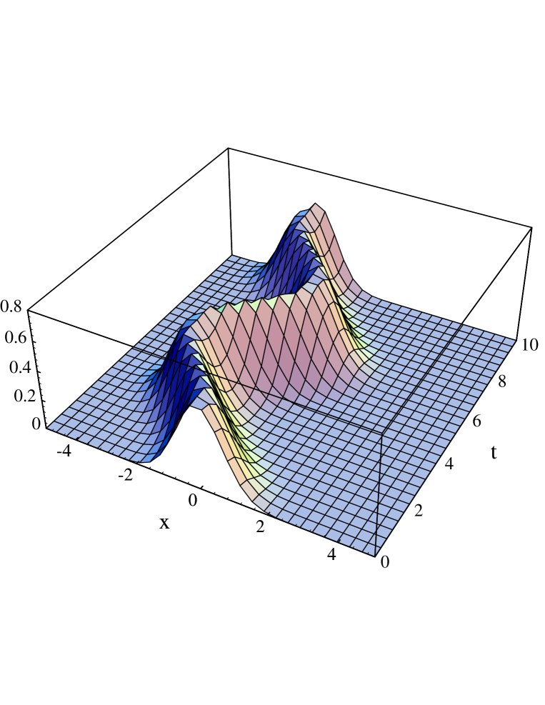
FIG. 1.: $w_{0}(x,t)$ for $\mu=1$ and $\nu=0$

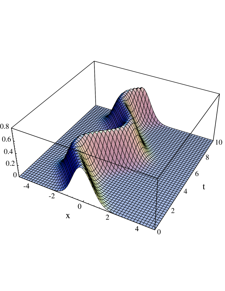
FIG. 2.: $w_{0}(x,t)$ for $\mu=1/\sqrt{2}$ and $\nu=1/\sqrt{2}$

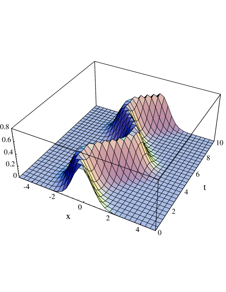
FIG. 3.: $w_{0}(x,t)$ for $\mu=0$ and $\nu=1$

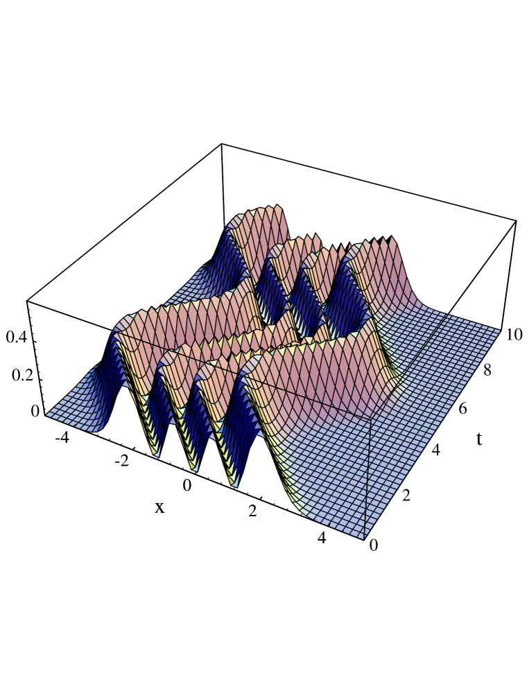
FIG. 4.: $w_{2}(x,t)$ for $\mu=1/\sqrt{2}$ and $\nu=1/\sqrt{2}$

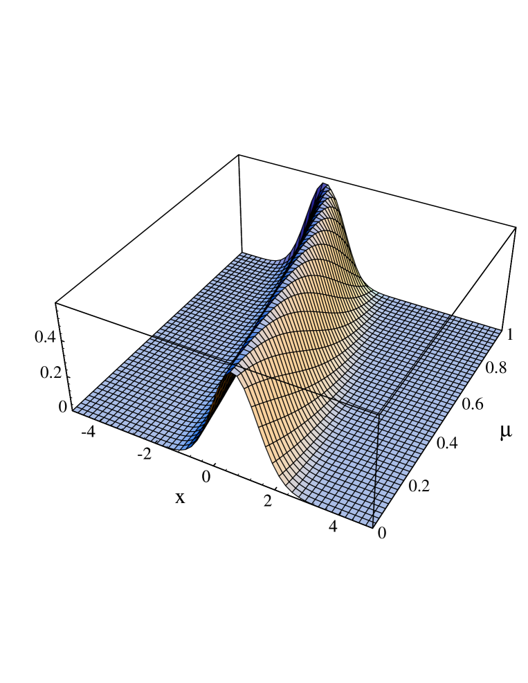
FIG. 5.: $w_{0}(x,4)$ for $\mu\in(0,1)$ and $\nu=\sqrt{1-\mu^{2}}$

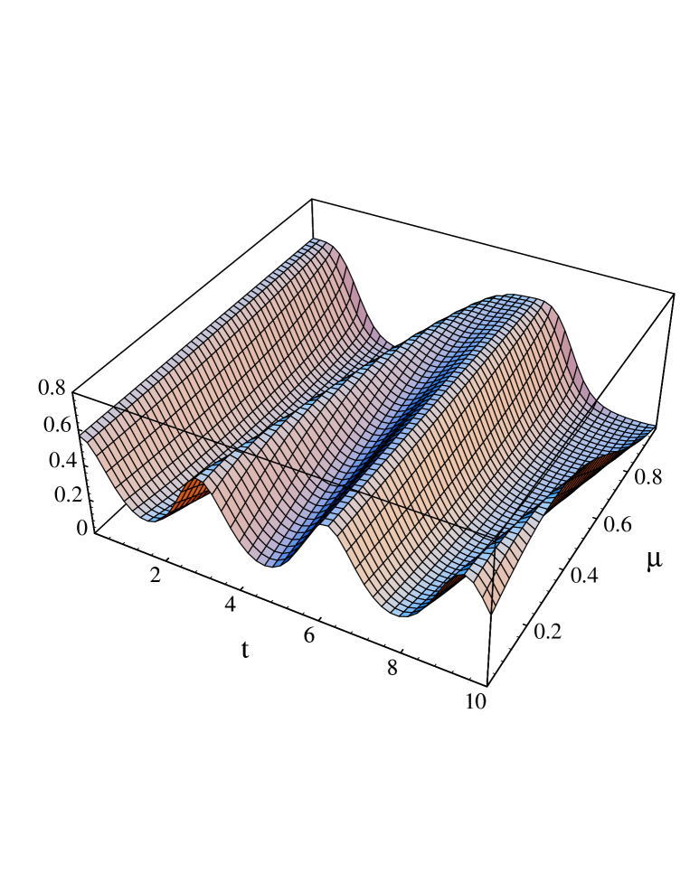
FIG. 6.: $w_{0}(0,t)$ for $\mu\in(0,1)$ and $\nu=\sqrt{1-\mu^{2}}$

REFERENCES

- [1] E. Schrödinger, Ann. Phys. (Leipzig), 79, 489 (1926).
- [2] L. D. Landau, Z. Physik, 45, 430 (1927).
- [3] J. von Neumann, Mathematische Grunlagen der Quantenmechanik (Springer, Berlin, 1932).
- [4] L. De Broglie, Compt. Rend., 183, 447 (1926); 184, 273 (1927); 185, 380 (1927).
- [5] D. Bohm, Phys. Rev., 85, 166; 180 (1952).
- [6] E. Wigner, Phys. Rev., 40, 749 (1932).
- [7] K. Husimi, Proc. Phys. Math. Soc. Jpn., 23, 264 (1940).
- [8] R. J. Glauber, Phys. Rev. Lett., 10, 84 (1963).
- [9] E. C. G. Sudarshan, Phys. Rev. Lett., 10, 277 (1963).
- [10] K. E. Cahill and R. J. Glauber, Phys. Rev., 177 1882 (1969).
- [11] J. E. Moyal, Proc. Cambridge Phylos. Soc.,45, 99 (1949).
- [12] S. Mancini, V. I. Man’ko, and P. Tombesi, Phys. Lett. A 213 1 (1996).
- [13] S. Mancini, V. I. Man’ko, and P. Tombesi, Found. Phys.27, 801 (1997).
- [14] S. Mancini, V. I. Man’ko, and P. Tombesi, Quantum Semiclass. Opt., 7, 615 (1995).
-
[15]
G. M. D’Ariano, S. Mancini, V. I. Man’ko, and P. Tombesi,
Quantum Semiclass. Opt., 8, 1017 (1996);
S. Mancini, V. I. Man’ko, and P. Tombesi, Europhys. Lett., 37, 79 (1997). - [16] V. I. Man’ko, “Optical symplectic tomography and classical probability instead of wave function in quantum mechanics,” in: GROUP21. Physical Applications and Mathematical Aspects of Geometry, Groups, and Algebras, Eds.: H.-D. Doebner, W. Scherer, and C. Schultz (World Scientific, Singapore, 1997), Vol. 2, p. 764; J. Russ. Laser Research, 17 579 (1996); “Quantum mechanics and classical probability theory,” in: Symmetries in Science IX, Eds.: B. Gruber and M. Ramek, Plenum Press, New York (1997), p. 215.
- [17] V. I. Man’ko and S. S. Safonov, Teor. Mat. Fiz., 112, 467 (1997)
- [18] O. V. Man’ko, J. Russ. Laser Research, 17, 439 (1996).
- [19] O. V. Man’ko and V. I. Man’ko, J. Russ. Laser Research, 18, 467 (1997).
-
[20]
Olga Man’ko, “Tomography of spin states and classical formulation
of quantum mechanics,” in: Symmetries in Science X, Eds.: B. Gruber
and M. Ramek, Plenum Press, New York (1998, to appear).
V. V. Dodonov and V. I. Man’ko Phys. Lett., A213, 1 (1997);
O. V. Man’ko and V. I. Man’ko JETP, 85, 430 (1997). - [21] J. Bertrand and P. Bertrand, Found. Phys., 17, 397 (1987).
- [22] K. Vogel and H. Risken, Phys. Rev., A40, 2847 (1989).
- [23] D. T. Smithey, M. Beck, M. G. Raymer, and A. Faridani, Phys. Rev. Lett., 70, 1244 (1993).
- [24] V. I. Man’ko, L. Rosa and P. Vitale Time–Dependent Invariants and Classical–like Description for the Quantum Parametric Oscillator, Napoli Preprint DSF-52/97.
-
[25]
H. R. Lewis Phys. Rev. Lett., 18, 510 (1967);
H. R. Lewis and W. Riesenfeld, J. Math. Phys., 10, 1458 (1969). -
[26]
V. V. Dodonov, I. A. Malkin, and V. I. Man’ko,
Int. J. Theo. Phys., 14, 37 (1975);
I. A. Malkin and V. I. Man’ko, Dynamical Symmetries and Coherent States of Quantum Systems, Nauka, Moscow (1979), [in Russian]. V. V. Dodonov and V. I. Man’ko, Invariants and Evolution of Nonstationary Quantum Systems, Proceedings of the Lebedev Physical Institute, Nova Science, New York (1989), Vol. 183. - [27] W. B. Campbell, P. Finkler, C. E. Jones, and M. N. Misheloff, Ann. Phys., 96, 286 (1976).
- [28] L. F. Urrutia and E. Hernandez, Int. J. Theo. Phys., 23, 1105 (1984).
- [29] G. Profilo and G. Soliani, Ann. Phys., 229, 160 (1994).
- [30] P. J. Bardroff, C. Leichte, G. Schrade, and W. P. Schleich, Phys. Rev. Lett., 77, 2198 (1996).
- [31] R. L. de Matos Filho, and W. Vogel, Phys. Rev., A 54, 4560 (1996).
- [32] V. I. Man’ko, G. Marmo, E. C. G. Sudarshan, and F. Zaccaria, Phys. Scripta, 55, 528 (1996).
- [33] R. P. Feynman and A. R. Hibbs Quantum Mechanics and Path Integrals McGraw-Hill Ed. (1965).
- [34] V. V. Dodonov, V. I. Man’ko, and D. E. Nikonov, Phys. Rev., A 51, 3328 (1995).
- [35] V. V. Dodonov, V. I. Man’ko, and L. Rosa,Phys. Rev. A, ??, ???? (1997).