Entanglement and visibility at the output of a Mach-Zehnder interferometer

Abstract

We study the entanglement between the two beams exiting a Mach-Zehnder interferometer fed by a couple of squeezed-coherent states with arbitrary squeezing parameter. The quantum correlations at the output are function of the internal phase-shift of the interferometer, with the output state ranging from a totally disentangled state to a state whose degree of entanglement is an increasing function of the input squeezing parameter. A couple of squeezed vacuum at the input leads to maximum entangled state at the output. The fringes visibilities resulting from measuring the coincidence counting rate or the squared difference photocurrent are evaluated and compared each other. Homodyne-like detection turns out to be preferable in almost all situations, with the exception of the very low signals regime.

I Introduction

The notion of entanglement is an essential feature of quantum mechanics, and is strictly connected with the nonlocal character of the theory. A two-part physical system prepared in an entangled state is described by a non factorizable density matrix. This gives raise to partial or total correlation between the outcomes of measurements performed on the two parts, even though the parts may be so far apart that no effects resulting from one measurement can reach the other part within the light cone.

Sources of entangled states are required for fundamentals tests of quantum mechanics, as well as for applications such as quantum computation and communication [1], and teleportation [2, 3]. In recent years, entangled photon pairs had been used to test non-locality of quantum mechanics [4, 5, 6, 7] by Bell inequality [8]. In practice, all the available sources of two-mode entangled states are based on the process of spontaneous down-conversion, taking place in $\chi^{(2)}$ nonlinear crystals [9]. Recently, it has been demonstrated that a beam splitter can split an incident photon into two correlated secondary photons [10, 11]. However, such process occurs at very low rate, and thus it is of no interest in practical applications.

In order to study quantum correlations between two radiation modes, and to compare different sources of correlated states, one needs to quantify the degree of entanglement [12]. A good theoretical measure of correlations has been introduced by means of Von-Neumann entropy. The entropy of a two-mode state $\hat{\varrho}$ is defined as

$$S[\hat{\varrho}]=-\hbox{Tr}\left\{\hat{\varrho}\log\hat{\varrho}\right\}\;,$$ (1)

whereas the entropies of the two modes $a$ and $b$ are given by

$$S[\hat{\varrho}_{a}]=-\hbox{Tr}_{a}\left\{\hat{\varrho}_{a}\log\hat{\varrho}_{a}\right\}\qquad S[\hat{\varrho}_{b}]=-\hbox{Tr}_{b}\left\{\hat{\varrho}_{b}\log\hat{\varrho}_{b}\right\}\;.$$ (2)

In Eq. (2) $\hat{\varrho}_{a}=\hbox{Tr}_{b}\left\{\hat{\varrho}\right\}$ and $\hat{\varrho}_{b}=\hbox{Tr}_{a}\left\{\hat{\varrho}\right\}$ denote the state of $a$ and $b$ respectively, as obtained by tracing out the other mode from the total density matrix. Following Refs. [12, 13, 14, 15] we define the degree of entanglement of the state $\hat{\varrho}$ as the normalized excess entropy [16]

$$\epsilon=\frac{1}{S[\hat{\varrho}_{a{\sc th}}]+S[\hat{\varrho}_{b{\sc th}}]}\Bigg{\{}S[\hat{\varrho}_{a}]+S[\hat{\varrho}_{b}]-S[\hat{\varrho}]\Bigg{\}}\;,$$ (3)

where $S[\hat{\varrho}_{\sc th}]=\log(1+N)+N\log(1+N^{-1})$, with $N=\langle a^{\dagger}a\rangle$, denotes the entropy of a thermal state, namely the maximally disordered state at fixed intensity. The use of $\epsilon$ formalizes the idea that the stronger are the correlations in the two-mode state, the more disordered should be the two modes taken separately. If $\hat{\varrho}$ is a pure state, we have that $S=0$ and $S_{a}=S_{b}$ [18], so that $\epsilon=S[\hat{\varrho}_{a}]/S[\hat{\varrho}_{a\sc th}]$ ranges from zero to unit. Notice that for pure state $\epsilon$ represents the unique measure of entanglement [17].

From the experimental point of view, the entanglement can be detected by non-classical interference effects occurring in intensity-dependent measurements. In experiments involving photon pairs from parametric down-conversion these effects occur when coincident photons are mixed at a beam splitter [19, 20, 21]. The probability amplitudes for pairs from the two arms show destructive interference, leading to a suppression of the coincidence counting rate between detectors surveying the two arms [22, 23]. Recently, the spatial effects in two-beam interference have been also studied for partially entangled photon pairs [24]. In the case of more excited states, many photons are present and the connection between entanglement and coincidence rate is less transparent. The issue has been received attention [25, 26], though a general theory has not been developed yet.

In this paper we study the generation and the detection of entangled states at the output of a Mach-Zehnder interferometer fed by a couple of uncorrelated squeezed-coherent states. The scheme may be of interest as the output state can be arbitrarily high excited, instead of having two photons only. In addition, the degree of entanglement can be tuned by varying the degree of squeezing of the input beams, or the internal phase shift of the interferometer. As regards the detection scheme, we show that the coincidence counting rate between the two output arms corresponds to low fringes visibility. Therefore, we consider instead another intensity dependent quantity, namely the squared difference photocurrent, which shows high visibility of fringes for the whole range of input squeezing parameter.

In Section II we study the dynamics of the interferometer, and evaluate analytically the degree of entanglement at the output as a function of the squeezing fraction of the input beams and the internal phase-shift of the interferometer. In Section III we analyze the interference effects occurring in the measurement of the photon coincidence rate and of the squared difference photocurrent. The evaluation of the fringes visibility for both measurements shows that homodyne-like detection is preferable in almost all situations, with the exception of the very low signals regime. Section IV closes the paper with some concluding remarks.

II Entanglement at the output of a Mach-Zehnder interferometer

The Mach-Zehnder interferometer we are dealing with is depicted in Fig. 1a. The input signal modes are denoted by $a$ and $b$, whereas $BS_{1}$ and $BS_{2}$ are symmetric beam splitters. We also assume that equal and opposite phase-shifts $\phi$ are imposed in each arm of the interferometer. The evolution operator of the whole setup can be written as

$$\hat{V}_{MZ}(\phi)=\hat{U}e^{i\phi(a^{\dagger}a-b^{\dagger}b)}\hat{U}^{\dagger}\;,$$ (4)

where

$$\hat{U}=\exp\left\{i\frac{\pi}{4}(a^{\dagger}b+b^{\dagger}a)\right\}\;,$$ (5)

denotes the evolution operator of a symmetric beam splitter. After straightforward algebra one rewrites Eq. (4) as

$$\hat{V}_{MZ}(\phi)=\exp\left\{i\frac{\pi}{2}b^{\dagger}b\right\}\exp\left\{-i\frac{\phi}{2}(a^{\dagger}b+b^{\dagger}a)\right\}\exp\left\{-i\frac{\pi}{2}b^{\dagger}b\right\}\;,$$ (6)

which shows that a Mach-Zehnder interferometer is equivalent to a single beam splitter $BS_{\phi}$ of transmissivity $\tau=\cos^{2}\frac{\phi}{2}$, preceded and followed by rotations of $\pi/2$ performed on one of the two modes (see Fig. 1b).

We consider the Mach-Zehnder interferometer fed by a couple of squeezed-coherent states

$$|\psi_{\sc in}\rangle\hat{D}_{a}(\alpha)\hat{D}_{b}(\alpha)\hat{S}_{a}(\zeta)\hat{S}_{b}(\zeta)|{\bf 0}\rangle=\;.$$ (7)

In Eq. (7) $\hat{D}_{a}(\alpha)=\exp(\alpha a^{\dagger}-\bar{\alpha}a)$ is the displacement operator and $\hat{S}(\zeta)=\exp[1/2(\zeta^{2}a^{{\dagger}2}-\bar{\zeta}^{2}a^{2})]$ is the squeezing operator, $|{\bf 0}\rangle$ denotes the electromagnetic vacuum. There is no need to consider a phase-shift between the input modes, as it can be reabsorbed into the internal phase shift $\phi$. Without loss of generality, in the following we will consider a complex field amplitude $\alpha\in{\mathbb{C}}$ and a real squeezing parameter $\zeta\equiv r\in{\mathbb{R}}$.

The state exiting the interferometer is given by

$$|\psi_{\sc out}\rangle=\hat{V}_{MZ}(\phi)\>|\psi_{\sc in}\rangle\;.$$ (8)

By exploiting the vacuum invariance $\hat{V}_{MZ}(\phi)|{\bf 0}\rangle=|{\bf 0}\rangle$ and using the relation

$$\exp\left\{-i\frac{\pi}{2}a^{\dagger}a\right\}\hat{D}(\alpha)\hat{S}(r)\exp\left\{i\frac{\pi}{2}a^{\dagger}a\right\}=\hat{D}(-i\alpha)\hat{S}(-r)\;,$$ (9)

we can write $|\psi_{\sc out}\rangle$ as

$$|\psi_{\sc out}\rangle=\exp\left\{i\frac{\pi}{2}b^{\dagger}b\right\}\>\>\hat{U}_{\phi}\hat{D}_{a}(\alpha)\hat{D}_{b}(-i\alpha)\hat{U}_{\phi}^{\dagger}\>\>\hat{U}_{\phi}\hat{S}_{a}(r)\hat{S}_{b}(-r)\hat{U}_{\phi}^{\dagger}\>\>|{\bf 0}\rangle\;,$$ (10)

where $\hat{U}_{\phi}$ denotes the evolution operator of the equivalent beam splitter $BS_{\phi}$. The ”displacing” part of Eq. (10), together with the rotation on the mode $b$, can be easily rewritten as

$$\exp\left\{i\frac{\pi}{2}b^{\dagger}b\right\}\hat{U}_{\phi}\hat{D}_{a}(\alpha)\hat{D}_{b}(-i\alpha)\hat{U}_{\phi}^{\dagger}=\hat{D}_{a}(\alpha e^{i\frac{\phi}{2}})\hat{D}_{b}(\alpha e^{\frac{i}{2}(\pi-\phi)})\exp\left\{i\frac{\pi}{2}b^{\dagger}b\right\}\;,$$ (11)

whereas the ”squeezing” part needs a little more algebra: specializing a result from Ref. [27] we can write

$$\hat{U}_{\phi}\hat{S}_{a}(r)\hat{S}_{b}(-r)\hat{U}_{\phi}^{\dagger}=\exp\left\{\cos\phi\left[\frac{1}{2}r(a^{{\dagger}2}-a^{2}-b^{{\dagger}2}+b^{2})\right]+\sin\phi\left[r(a^{\dagger}b^{\dagger}-ab)\right]\right\}\;.$$ (12)

It is worth noting that squeezing at the input is essential to obtain entanglement at the output. In fact, for the input state being a couple of coherent states $|\psi_{\sc in}\rangle=\hat{D}_{a}(\alpha)\hat{D}_{b}(\beta)|{\bf 0}\rangle$ the output state is given by $|\psi_{\sc out}\rangle=\hat{D}_{a}(\alpha\cos\phi-i\beta\sin\phi)\hat{D}_{b}(-i\alpha\sin\phi+\alpha\cos\phi)|{\bf 0}\rangle$, which again is a couple of factorized (uncorrelated) coherent states for any value of the internal phase-shift of the interferometer. Actually, the absence of output correlations is due the the Poissonian statistics of the coherent states, which implies the absence of intensity fluctuations [28].

Let us first consider the situation $\phi=\frac{\pi}{2}$. In this case, the transformation in Eq. (12) reduces to the two-mode squeezing operator $\hat{S}^{(2)}(r)=\exp\left\{r(a^{\dagger}b^{\dagger}-ab)\right\}$, so that the output state coincides with a displaced and rotated twin-beam state

$$|\psi_{\sc out}\rangle=\hat{D}_{a}(\alpha e^{i\frac{\phi}{2}})\hat{D}_{b}(\alpha e^{\frac{i}{2}(\pi-\phi)})\exp\left\{i\frac{\pi}{2}b^{\dagger}b\right\}|\psi_{\sc twb}\rangle\;,$$ (13)

where the explicit expression of the twin-beam state $|\psi_{\sc twb}\rangle$ is given by

$$|\psi_{\sc twb}\rangle=\hat{S}^{(2)}(r)|{\bf 0}\rangle=\frac{1}{\cosh r}\sum_{k=0}^{\infty}\tanh^{k}r\>|k,k\rangle\;.$$ (14)

In order to evaluate the degree of entanglement of $|\psi_{\sc out}\rangle$ we use the parameter $\epsilon$ introduced in Eq. (3). The partial trace over a mode, say $b$, is given by

$$\hat{\varrho}_{a}=\hbox{Tr}_{b}\left\{|\psi_{\sc out}\rangle\langle\psi_{\sc out}|\right\}=\frac{1}{\cosh^{2}r}\sum_{k=0}^{\infty}\tanh^{2k}r\>\hat{D}(\alpha e^{i\frac{\pi}{4}})|k\rangle\langle k|\hat{D}^{\dagger}(\alpha e^{i\frac{\pi}{4}})\;,$$ (15)

which is diagonal in the basis of displaced number states $|\psi_{n}\rangle=\hat{D}(\alpha e^{i\frac{\pi}{4}})|n\rangle$. The set of $|\psi_{n}\rangle$’s constitutes an orthogonal basis for the Hilbert space of harmonic oscillator, and therefore the entropy $S[\hat{\varrho}_{a}]$ can be evaluated as

$$S[\hat{\varrho}_{a}]=-\sum_{n=0}^{\infty}p_{n}\log p_{n}\qquad p_{n}=\frac{1}{\cosh^{2}r}\tanh^{2n}r\;.$$ (16)

After straightforward calculation we arrive at

$$S[\hat{\varrho}_{a}]=\log(1+\nu^{2})+\nu^{2}\log(1+\frac{1}{\nu^{2}})\;,$$ (17)

where $\nu^{2}=\sinh^{2}r$ is the squeezing energy of each input beam. Notice that $S[\hat{\varrho}_{a}]$ in Eq. (17) is equivalent to the entropy of a thermal state with $\nu^{2}$ photons. The degree of entanglement is given by

$$\epsilon=\frac{\log(1+\gamma N)+\gamma N\log(1+\frac{1}{\gamma N})}{\log(1+N)+N\log(1+\frac{1}{N})}\;,$$ (18)

where $N=\langle a^{\dagger}a\rangle=|\alpha|^{2}+\nu^{2}$ is the total energy of each input signal, and $\gamma$ is the squeezing fraction, namely the percentage of the total energy engaged in squeezing photons, $\nu^{2}=\gamma N$. From Eq. (18) it is apparent that the degree of entanglement is an increasing function of the squeezing fraction, and that the maximum entangled state ($\epsilon=1$) at the output is reached for a couple of squeezed vacuum ($\gamma=1$) at the input.

For $\phi=0$, the transmissivity of the whole device is equal to unit, and we have $|\psi_{\sc out}\rangle=|\psi_{\sc in}\rangle$. Therefore, the entanglement is equal to zero, as the input state consists of a couple of uncorrelated signals.

For $\phi\neq 0,\frac{\pi}{2}$ it is convenient to evaluate the output state and the entanglement by evolving the two-mode Wigner function, which is defined as follows

$$W(x_{a},y_{a};x_{b},y_{b}) = \int_{\mathbb{R}}\!\!d\mu_{a}\int_{\mathbb{R}}\!\!d\nu_{a}\int_{\mathbb{R}}\!\!d\mu_{b}\int_{\mathbb{R}}\!\!d\nu_{b}\>\exp\left\{2i(\nu_{a}x_{a}-\mu_{a}y_{a}+\nu_{b}x_{b}-\mu_{b}y_{b})\right\}\times$$ (19)

$$\times \hbox{Tr}\left\{\hat{\varrho}\>\hat{D}_{a}(\mu_{a}+i\nu_{a})\hat{D}_{b}(\mu_{b}+i\nu_{b})\right\}\;.$$ (20)

The $\pm\pi/2$ rotations of mode $b$ correspond to simple rotations in the sole $b$-variables

$$\hat{\varrho}^{\prime} = e^{i\frac{\pi}{2}}\hat{\varrho}\>e^{-i\frac{\pi}{2}}\qquad\Longrightarrow\qquad W^{\prime}(x_{a},y_{a};x_{b},y_{b})=W(x_{a},y_{a};y_{b},-x_{b})$$ (21)

$$\hat{\varrho}^{\prime} = e^{-i\frac{\pi}{2}}\hat{\varrho}\>e^{i\frac{\pi}{2}}\qquad\Longrightarrow\qquad W^{\prime}(x_{a},y_{a};x_{b},y_{b})=W(x_{a},y_{a};-y_{b},x_{b})\;,$$ (22)

whereas the action of the beam splitter $BS_{\phi}$, i.e. $\hat{\varrho}^{\prime}=\hat{U}_{\phi}\hat{\varrho}\hat{U}_{\phi}^{\dagger}$ corresponds to a mixing of variables of the two modes, in formula

$$W^{\prime}(x_{a},y_{a};x_{b},y_{b})=W( x_{a}\cos\delta-x_{b}\sin\delta,y_{a}\cos\delta-y_{b}\sin\delta;$$ (24)

$$x_{a}\sin\delta+x_{b}\cos\delta,y_{a}\sin\delta+y_{b}\cos\delta)\;,$$

where we use the notation $\delta=\phi/2$. Using Eqs. (22) and (24) the Wigner function at the output results

$$W_{\sc out}(x_{a},y_{a};x_{b},y_{b})=W_{\sc in}( x_{a}\cos\delta-y_{b}\sin\delta,y_{a}\cos\delta+x_{b}\sin\delta;$$ (26)

$$x_{b}\cos\delta-y_{b}\sin\delta,x_{a}\sin\delta+y_{b}\cos\delta)\;,$$

where $W_{\sc IN}(x_{a},y_{a};x_{b},y_{b})$ is a product of two identical single-mode Gaussian Wigner functions, corresponding to the couple of input squeezed-coherent states:

$$W_{\sc in}(x_{a},y_{a};x_{b},y_{b})=\frac{4}{\pi^{2}}\exp\Bigg{\{} - 2e^{-2r}(x_{a}-\hbox{Re}[\alpha])^{2}-2e^{2r}(y_{a}-\hbox{Im}[\alpha])^{2}$$ (27)

$$- 2e^{-2r}(x_{b}-\hbox{Re}[\alpha])^{2}-2e^{2r}(y_{b}-\hbox{Im}[\alpha])^{2}\Bigg{\}}\;.$$ (28)

By the integration over the $b$-variables

$$W_{\sc out}(x_{a},y_{a})=\int_{\mathbb{R}}\!\!dx_{b}\int_{\mathbb{R}}\!\!dy_{b}\>W_{\sc out}(x_{a},y_{a};x_{b},y_{b})\;,$$ (29)

and inserting Eqs. (26) and (28) in Eq. (29) we obtain

$$W_{\sc out}(x_{a},y_{a})=\frac{1}{\pi\Sigma_{x}\Sigma_{y}}\exp\left\{-\frac{(x_{a}-\hbox{Re}[\alpha_{\phi}])^{2}}{\Sigma_{x}^{2}}-\frac{(y_{a}-\hbox{Im}[\alpha_{\phi}])^{2}}{\Sigma_{y}^{2}}\right\}\;,$$ (30)

which represents the Wigner function of the sole mode $a$ after partial trace over the mode $b$. The quantities $\Sigma_{x}$ and $\Sigma_{y}$ in Eq. (30) are given by

$$\Sigma_{x}^{2} = e^{2r}\cos^{2}\delta+e^{-2r}\sin^{2}\delta$$ (31)

$$\Sigma_{y}^{2} = e^{-2r}\cos^{2}\delta+e^{2r}\sin^{2}\delta\;,$$ (32)

whereas $\alpha_{\phi}$ is given by

$$\alpha_{\phi}=\alpha\sqrt{1+\frac{1}{2}\sin^{2}\phi}\;.$$ (33)

In order to evaluate entanglement, we note that any unitary transformation $\hat{T}$ acting on the single mode $a$ does not change the value of the entropy [25], i.e. $S[\hat{\varrho}_{a}]=S[\hat{T}\hat{\varrho}_{a}\hat{T}^{\dagger}]$. Using this property, we displace with amplitude $\alpha_{\phi}$, and then squeeze with parameter $r^{\ast}=\log\sqrt{\Sigma_{y}/\Sigma_{x}}$ the Wigner function in Eq. (30), thus arriving at the following entropy-equivalent state

$$W^{\prime}_{\sc out}(x_{a},y_{a})=\frac{1}{\pi\Sigma_{x}\Sigma_{y}}\exp\left\{-\frac{x_{a}^{2}+y_{a}^{2}}{\Sigma_{y}\Sigma_{x}}\right\}\;.$$ (34)

Remarkably, the Wigner function in Eq. (34) coincides with the Wigner function of a thermal states with thermal photons given by

$$N_{\phi}=\frac{1}{2}\left[\Sigma_{y}\Sigma_{x}-1\right]=\frac{1}{2}\left[\sqrt{1+\sin^{2}\phi\sinh^{2}2r}-1\right]\;.$$ (35)

The corresponding entropy can be easily computed, and thus the entanglement at the output is given by

$$\epsilon=\frac{\log(1+N_{\phi})+N_{\phi}\log(1+\frac{1}{N_{\phi}})}{\log(1+N)+N\log(1+\frac{1}{N})}\;.$$ (36)

As it is expected, one has $N_{\phi}=0$ for $\phi=0$, and $N_{\phi}=\gamma N$ for $\phi=\pi/2$.

In Fig. 2a we show the degree of entanglement as a function of the squeezing fraction $\gamma$ and the internal phase-shift $\phi$, in the case of input beams with average photons $N=3$ each: at fixed $\gamma$ the output state ranges from a totally disentangled state for $\phi=0$, to a state whose degree of entanglement is given by Eq. (18) for $\phi=\frac{\pi}{2}$. The degree of entanglement is an increasing function of the squeezing fraction $\gamma$, with the condition $\phi=\frac{\pi}{2}$ corresponding to maximum value. Different values of the intensity $N$ does not substantially modify the behavior of $\epsilon$ versus $\gamma$ and $\phi$. In Fig. 2b we report $\epsilon$ as a function of the intensity $N$ for different values of the squeezing fraction $\gamma$, and for fixed value $\phi=\frac{\pi}{2}$ of the internal phase-shift: For $\gamma=1$ one has $\epsilon=1$ independently on $N$, whereas for $\gamma<1$ the degree of entanglement becomes a slightly increasing function of $N$. For highly excited states the entanglement is given by the asymptotic formula

$$\epsilon\stackrel{{\scriptstyle N\gg 1}}{{\simeq}}1+\frac{\log\gamma}{\log N}\;.$$ (37)

So far we have considered the two input states having the same degree of squeezing. However, a pair of input states with different squeezing fractions does not substantially modify the picture. In this case, in fact, the entanglement still oscillates from $\epsilon=0$ to a maximum value as a function of the internal phase-shift of the interferometer. On the other hand, this maximum value is now a function of both the squeezing fractions, and maximally entangled states at the output cannot be achieved if one of the input signals is only partially squeezed. In Fig. 3 we report the maximum entanglement at the output (obtained for $\phi=\pi/2$) as a function of the squeezing fractions $\gamma_{1}$ of one of the beams for different values of the squeezing fraction $\gamma_{2}$ of the other beam. The plots refers to a situation in which both input beams have an average number of photons equal to $N=3$. As it is apparent from the plots, the output entanglement is an increasing function of both the two squeezing fractions. The extreme case in which one of the input signals is no squeezed at all corresponds to a value of $\epsilon$ always lower than $50\%$.

III Entanglement and fringes visibility

In this Section, we study the visibility of the interference fringes that are observed, by varying the internal phase-shift $\phi$, in intensity measurements at the output of the interferometer. In analogy with experiments involving correlated photon pairs, we consider the detection of the coincidence counting rate at the output, namely of the fourth-order correlation function $\langle\psi_{\sc out}|a^{\dagger}a\>b^{\dagger}b|\psi_{\sc out}\rangle$. However, as we will show in the following, this corresponds to low fringes visibility, and thus we sought for a more sensitive kind of measurement. The homodyne-like detection of the output difference photocurrent $\langle\psi_{\sc out}|a^{\dagger}a-b^{\dagger}b|\psi_{\sc out}\rangle$ is widely used in interferometry [29, 30, 31], and generally results in a very sensitive measurement scheme. Starting from this consideration, we suggest the squared difference photocurrent $\langle\psi_{\sc out}|(a^{\dagger}a-b^{\dagger}b)^{2}|\psi_{\sc out}\rangle$ as a suitable fourth-order quantity to be measured at the output of the interferometer.

Besides being originated by interference effects, the variations in the quantities measured at the output also reflect the variations in the quantum correlations between the two output signals. Therefore, the visibility of the interference fringes provides a measure of entanglement, and comparing the visibility of different measurement schemes provides a way to compare their ability in monitoring the variations of quantum correlations between the output signals.

As already mentioned, here we consider the measurement of the coincidence counting rate

$$K(\phi)=\langle\psi_{\sc out}|a^{\dagger}a\>b^{\dagger}b|\psi_{\sc out}\rangle=\langle\psi_{\sc in}|\hat{V}_{MZ}^{\dagger}(\phi)a^{\dagger}a\>b^{\dagger}b\>\hat{V}_{MZ}(\phi)|\psi_{\sc in}\rangle\;,$$ (38)

and of the squared difference photocurrent

$$H(\phi)=\langle\psi_{\sc out}|(a^{\dagger}a-b^{\dagger}b)^{2}|\psi_{\sc out}\rangle=\langle\psi_{\sc in}|\hat{V}_{MZ}^{\dagger}(\phi)(a^{\dagger}a-b^{\dagger}b)^{2}\>\hat{V}_{MZ}(\phi)|\psi_{\sc in}\rangle\;.$$ (39)

After some algebra, we arrive at the explicit expressions in terms of the input fields

$$\hat{K}(\phi) = \hat{V}_{MZ}^{\dagger}(\phi)a^{\dagger}a\>b^{\dagger}b\>\hat{V}_{MZ}(\phi)=$$ (40)

$$= \sin^{2}\delta\cos^{2}\delta\left[a^{{\dagger}2}a^{2}+b^{{\dagger}2}b^{2}+a^{{\dagger}2}b^{2}+b^{{\dagger}2}a^{2}\right]+(\sin^{2}\delta-\cos^{2}\delta)^{2}a^{\dagger}a\>b^{\dagger}b+$$ (41)

$$+ i\sin\delta\cos^{3}\delta\left[ab^{{\dagger}2}b+a^{{\dagger}2}ab-a^{\dagger}b^{\dagger}b^{2}-a^{\dagger}a^{2}b^{\dagger}\right]+$$ (42)

$$+ i\sin^{3}\delta\cos\delta\left[a^{\dagger}a^{2}b^{\dagger}+a^{\dagger}b^{\dagger}b^{2}-a^{{\dagger}2}ab-ab^{{\dagger}2}b\right]\;,$$ (43)

$$\hat{H}(\phi) = \hat{V}_{MZ}^{\dagger}(\phi)(a^{\dagger}a-b^{\dagger}b)^{2}\>\hat{V}_{MZ}(\phi)=-2\hat{K}(\phi)+$$ (44)

$$+ \left[(a^{\dagger}a)^{2}+(b^{\dagger}b)^{2}\right](\sin^{4}\delta+\cos^{4}\delta)-2\sin^{2}\delta\cos^{2}\delta\left[a^{{\dagger}2}b^{2}+b^{{\dagger}2}a^{2}-a^{\dagger}a-b^{\dagger}b\right]+$$ (45)

$$+ 2i\sin\delta\cos^{3}\delta\left[a^{\dagger}a^{2}b^{\dagger}-a^{{\dagger}2}ab+a^{\dagger}b^{\dagger}b^{2}-ab^{{\dagger}2}b\right]+$$ (46)

$$+ 2i\sin^{3}\delta\cos\delta\left[ab^{{\dagger}2}b-a^{\dagger}b^{\dagger}b^{2}+a^{{\dagger}2}ab-a^{\dagger}a^{2}b^{\dagger}\right]\;,$$ (47)

where again we used the notation $\delta=\frac{\phi}{2}$. Using Eqs. (43) and (47) we are able to evaluate the fringes visibility of both detection schemes

$$V_{K}=\frac{K_{max}-K_{min}}{K_{max}+K_{min}}\qquad V_{H}=\frac{H_{max}-H_{min}}{H_{max}+H_{min}}\;.$$ (48)

In Fig. 4 we report $V_{K}$ and $V_{H}$ as a function of the intensity $N$ for different values of the input squeezing fraction $\gamma$. The H-measurement visibility $V_{H}$ is larger than $V_{K}$ in almost all situations, with the exception of the very low signals regime, where very few photons are present. The behavior of fringes visibility versus intensity $N$ also confirms that $V_{H}$ represents a good measure of the entanglement at the output. As it happens for the degree of entanglement, in fact, a couple of squeezed vacuum at the input corresponds to maximum visibility $V_{H}=1$ independently on the intensity,. On the other hand, the coincidence counting rate shows a visibility $V_{K}$ that rapidly decreases versus $N$, and saturates to a value well below $1/2$. For non unit squeezing fraction, and moderate input intensities $N<10$, the behavior of $V_{H}$ looks qualitatively similar to that of the degree of entanglement (compare Fig. 4b and Fig. 2b), whereas again $V_{K}$ rapidly decreases. Remarkably, for highly excited states $N>10$, the visibility $V_{H}$ has the same asymptotic dependence of the degree of entanglement $\epsilon$, in formula

$$\epsilon\stackrel{{\scriptstyle N\gg 1}}{{\simeq}}1+\frac{A(\gamma)}{\log N}\;,$$ (49)

where the proportionality constant $A(\gamma)\simeq 1/5\log\gamma$ is roughly proportional to that appearing in Eq. (37).

IV Conclusions

The generation and the detection of optical entangled states are important issues, both required for fundamentals tests of quantum mechanics, as well as for possible applications. In this paper we have studied the entanglement between the two beams exiting a Mach-Zehnder interferometer fed by a couple of squeezed-coherent states with arbitrary squeezing parameter. The degree of entanglement at the output has been analytically evaluated, as a function of the input intensity and squeezing fraction, and of the internal phase-shift of the interferometer. Our results indicate that entangled states of arbitrary large intensity can be produced by varying the input energy, whereas the degree of entanglement can be tuned by varying the input squeezing fraction, and the internal phase-shift.

An experimental characterization of the output entanglement can be obtained through the measurement of the squared difference photocurrent between the output modes. The interference fringes that are observed by varying the internal phase-shift $\phi$ show, in fact, high visibility for the whole range of input squeezing parameter.

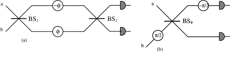
FIG. 1.: In (a): schematic diagram of a Mach-Zehnder interferometer. $BS_{1}$ and $BS_{2}$ are symmetric beam splitters, whereas $a$ and $b$ denote the input signal modes. Equal and opposite phase-shifts are imposed in each arm. In (b): an equivalent scheme for the Mach-Zehnder interferometer depicted in (a): a single beam splitter $BS_{\phi}$ of transmissivity $\tau=\cos^{2}\frac{\phi}{2}$ preceded and followed by rotations of $\frac{\pi}{2}$ performed on one of the two modes (here $b$).

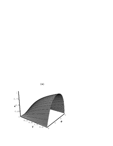
FIG. 2.: (a):the degree of entanglement as a function of the squeezing fraction $\gamma$ and the internal phase-shift $\phi$, in the case of input beams with $N=3$ each: for fixed $\gamma$ the output state ranges from a totally disentangled state for $\phi=0$, to a state with a degree of entanglement given by Eq. (18) for $\phi=\frac{\pi}{2}$. The degree of entanglement is an increasing function of $\gamma$, with $\phi=\frac{\pi}{2}$ corresponding to maximum value. Different values of $N$ do not substantially modifies the picture. (b): the degree of entanglement as a function of the total input energy $N$ for different values of the squeezing fraction $\gamma$, and for fixed value $\phi=\frac{\pi}{2}$ of the internal phase-shift.

FIG. 3.: Output entanglement for input signals with different degree of squeezing. The maximum entanglement at the output (for $\phi=\pi/2$) is reported as a function of the squeezing fractions $\gamma_{1}$ of one of the beams for different values of the squeezing fraction $\gamma_{2}$ of the other beam. Both input beams have an average number of photons equal to $N=3$. The output entanglement is an increasing function of both the two squeezing fractions. The extreme case in which one of the input signals is no squeezed at all corresponds to a value of $\epsilon$ always lower than $50\%$.

FIG. 4.: Fringes visibility as a function of the intensity $N$ for different values of the input squeezing fraction $\gamma$. In (a) the visibility of K-measurement $V_{K}$, and in (b) the visibility of H-measurement $V_{H}$ . In both plots we report the visibility versus $N$ for five values of the input squeezing fraction. From bottom to top we have the curves for $\gamma=0.2,0.4,0.6,0.8,\hbox{and }1.0$. As it is apparent, $V_{H}$ is larger than $V_{K}$ in almost all situations, with the exception of the very low signals regime.

REFERENCES

• [1] C. H. Bennet, Phys. Today, 48, 24 (1995); C. H. Bennett, D. P. Di Vincenzo, Nature 377, 389 (1995).
• [2] D. Boschi, S. Branca, F. De Martini, L. Hardy, S. Popescu, Phys. Rev. Lett. 80, 1121 (1998).
• [3] S. L. Braunstein, H. J. Kimble, Phys. Rev. Lett. 80, 869 (1998).
• [4] Z. Y. Ou, L. Mandel, Phys. Rev. Lett. 61, 50 (1988).
• [5] J. G. Rarity, P. R. Tapster, Phys. Rev. Lett. 64, 2495 (1990).
• [6] M. H. Rubin, Y. H. Shih, Phys. Rev. A 45, 8138 (1992).
• [7] P. G. Kwiat, K. Mattle, H. Weinfurther, A. Zeilinger, Phys. Rev. Lett. 75, 4337 (1995).
• [8] J. S. Bell Physics 1, 195 (1964).
• [9] D. N. Klyshko, Photons and Nonlinear Optics, (Gordon and Breach, New York, 1988).
• [10] J. D. Franson, Phys. Rev. A 53, 3756 (1996).
• [11] J. D. Franson, Phys. Rev. A 56, 1800 (1997).
• [12] S. M. Barnett, S. J. D. Phoenix, Phys. Rev. A 44, 535 (1991).
• [13] G. Lindblad, Comm. Math. Phys. 33, 305 (1973).
• [14] S. M. Barnett, S. J. D. Phoenix, Phys. Rev. A 40, 2404 (1989).
• [15] V. Vedral, M. B. Plenio, K. Jacobs, P. L. Knight, Phys. Rev. A 56, 4452 (1997).
• [16] Our definition slightly differs from that of Refs. [12, 13, 14], where no normalization to a thermal state was used.
• [17] S. Popescu, D. Rohrlich, Phys. Rev. A 56, R3319 (1997).
• [18] H. Araki, E. H. Lieb, Comm. Math. Phys. 18, 160 (1970).
• [19] C. K. Hong, Z. Y. Ou, L. Mandel, Phys. Rev. Lett. 59, 2044 (1987).
• [20] L. Mandel, Opt. Lett. 16, 1882 (1991).
• [21] J. G. Rarity, P. R. Tapster, Phys. Rev. A 45, 2052 (1992).
• [22] H. Fearn, R. Loudon, Opt. Comm. 64, 485 (1987).
• [23] H. Fearn, R. Loudon, J. Opt. Soc. Am. B 6, 917 (1989).
• [24] B. E. A. Saleh, A. Joobeur, M. C. Teich, Phys. Rev. A 57, 3991 (1998).
• [25] B. Böhmer, U. Leonhardt, Opt. Comm. 118, 181 (1995).
• [26] G. Di Giuseppe, L. Haiberger, F. De Martini, A. V. Sergienko, Phys. Rev. A 56, R21 (1997).
• [27] M. G. A. Paris Phys. Lett. A 225, 28 (1997).
• [28] L. Mandel, E. Wolf Optical Coherence and Quantum Optics (Cambridge University Press, 1995) pag. 642-644.
• [29] C. M. Caves, Phys. Rev. D 23, 1693 (1981).
• [30] R. S. Bondurant and J. H. Shapiro, Phys. Rev. A 30, 2548 (1984).
• [31] M. G. A. Paris, Phys. Lett A 201, 132 (1995).
Refer to caption