Optimization approach to entanglement distillation

Abstract

We put forward a method for optimized distillation of partly entangled pairs of qubits into a smaller number of more entangled pairs by recurrent local unitary operations and projections. Optimized distillation is achieved by minimization of a cost function with up to 30 real parameters, which is chosen to be sensitive to the fidelity and the projection probability at each step. We show that in many cases this approach can significantly improve the distillation efficiency in comparison to the present methods.

I Introduction

Entanglement distillation or purification [1, 2, 3, 4, 5] denotes the extraction of strongly entangled pairs of qubits from a larger number of weakly entangled pairs. The objective is to share strongly correlated qubits between distant parties in order to allow reliable quantum teleportation [6] or quantum cryptography [7]. All methods of entanglement purification require that the two parties perform only local operations on their systems and that only classical information be exchanged between them, without transferring any additional qubits. The possible local operations include (Fig. 1): (i) unitary transformations whereby each party entangles the particles at their disposal; (ii) non-unitary projections, whereby each party measures a portion of their particles, thus projecting the rest of the system onto a new state. These projections are usually followed by classical communication of the measurement results between the parties. Another non-unitary operation is filtering [5], whereby a pair is with a certain probability either discarded or kept after each projection, the probability being dependent on the state.

The principles of the known distillation schemes have been surveyed in [2]. Here we focus on recurrence distillation methods which use two pairs of qubits as input and produce a single output pair: (a) The quantum privacy amplification (QPA) method [3] requires that the projection of the input pairs on any of the four states of the Bell basis ($|\psi^{\pm}\rangle$ = $2^{-1/2}$ $(0,1,\pm 1,0)^{{\dagger}}$ and $|\phi^{\pm}\rangle$ = $2^{-1/2}$ $(1,0,0,\pm 1)^{{\dagger}}$) be larger than 1/2. The QPA method uses a sequence of $\pi/2$ rotations, controlled-not operations and measurements. (b) In the method of Ref. [1] the two-qubit input state is supposed to have a projection larger than 1/2 on the singlet state $|\psi^{-}\rangle$. This method uses a sequence of unilateral $\pi$ rotations of the qubits and a bilateral XOR operation followed by a measurement. The output is a pair whose projection on the singlet state is larger than that of the input pair. When used recurrently, the QPA method [3] often converges faster towards a Bell state than the method of [1] (for the proof of convergence of the QPA see [4]).

FIG. 1.: Stages of the basic entanglement purification scheme: (I) The two parties A and B share two partly entangled pairs $\varrho_{1}$ and $\varrho_{2}$, (II) they apply local unitary transforms $U_{a}$ and $U_{b}$, and, (III) project out one of the pairs, thus obtaining the remaining pair in the state $\varrho$.

Both of the aforementioned recurrence methods use fixed parameters for the state transformations. It is not clear whether these methods are optimal for the states which are usable as their input, and, if not, how can their performance be improved. There are other states for which these methods do not work at all. This is demonstrated in Fig. 2, which gives the statistics of applicability of the QPA method for randomly chosen two-qubit states. The random two-qubit density matrices were generated as in Ref. [8] and the statistics was obtained from a sample of $10^{6}$ trials [9]. For each of the generated density matrices it was checked whether it corresponds to an entangled (i.e., inseparable) state, and, if so, whether it can be purified by the QPA. The results show that about 37% of all the possible states are entangled and in principle can be used for entanglement distillation. About 74% of the entangled states have fidelity (see Sec. II B) [2] $F>1/2$ and in principle can, after appropriate manipulations, be used for the QPA. Only a 12% fraction of the inseparable states, which is about 4% of the sample, have a diagonal density-matrix element larger than 1/2 in the Bell basis, and can therefore be used directly as the input of the QPA algorithm. This suggests that there is a vast domain in the space of two-qubit states where new approaches to the distillation problem can be useful.

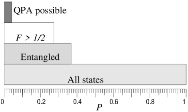
FIG. 2.: Statistics of the entanglement properties of an ensemble of randomly chosen two-qubit states. The areas of the rectangles (from bottom to top) are proportional to the following probabilities: the entire ensemble (All states), the probability that a randomly chosen state is entangled, the probability that it fulfills the condition $F$ $>$ $1/2$, and the probability that it is directly usable as an input of the QPA scheme (QPA possible).

Here we deal with entanglement distillation as a problem of optimization, aimed at improving the efficiency of the recurrence methods and extending the class for which they work. In contrast to the previously discussed recurrence methods, we assume that the transformation parameters can be chosen at will to our advantage. Furthermore, as opposed to the ingenious choice of parameters in these methods, we do not have to guess their values: the optimal choice of parameters for the unitary operations and the projections is obtained by minimization of an approximate cost function, which represents a tradeoff between maximized probability of the conditional measurement and the best achievable entanglement. These principles are similar to the ones previously used for optimized state engineering [10]. However, the present task is still nontrivial, since the number of control parameters is large (up to 30), and the choice of a cost function is far from obvious.

These issues are analyzed in Sec. II, where the optimization procedure is obtained. This procedure is then applied in Sec. III to cases where the QPA is inefficient, to input states with fidelity $F$ $<$ 1/2, and to trapped ion qubits. The results are discussed in Sec. IV.

II Optimization procedure

Let us assume that we want to prepare, starting from two pairs of qubits with density matrices $\varrho_{1}$ and $\varrho_{2}$, a single pair with a density matrix $\varrho$ whose entanglement is larger than that of both $\varrho_{1}$ and $\varrho_{2}$, using local unitary transformations followed by projections (Fig. 1). Let us denote the local unitary transforms of each party by $U_{a}$ and $U_{b}$, respectively. If the measurements are performed on the particles of the second pair, with the detected state being $|\Psi\rangle_{2}$, then the first (purified) pair is transformed into the state

$$\varrho=\frac{1}{P}~{}_{2}\langle\Psi|U_{a}U_{b}\varrho_{1}\otimes\varrho_{2}U_{b}^{{\dagger}}U_{a}^{{\dagger}}|\Psi\rangle_{2},$$ (1)

$P$ being the probability of success,

$$P={\rm Tr}\ _{2}\langle\Psi|U_{a}U_{b}\varrho_{1}\otimes\varrho_{2}U_{b}^{{\dagger}}U_{a}^{{\dagger}}|\Psi\rangle_{2}.$$ (2)

Provided that each particle is a two-level system, the two-particle unitary transformation of each party belongs to the SU(4) group (considering SU(4) instead of U(4) means that we omit the unimportant overall phase). Such a group has 15 real parameters. The local transformations on both sides are thus parametrized with 30 real parameters. Finding the optimum values for these 30 parameters would enable us to perform the entanglement distillation in the most efficient way. For this purpose, we must (i) find a proper parametrization of the transformations, (ii) choose a function that quantifies the success of the distillation, and (iii) have a suitable method for the optimization of this function.

A Parametrization of the local unitary transformations

To parametrize the SU(4) local unitary transformations, we use a modified version of the scheme in Ref. [11], in the form of a product of six SU(2) transformations:

$$U= U^{(1,2)} (\phi_{12},\psi_{12},\chi_{12})$$ (3)

$$\times U^{(2,3)} (\phi_{23},0,\chi_{23})U^{(1,3)}(\phi_{13},\psi_{13},\chi_{13})$$ (4)

$$\times U^{(3,4)} (\phi_{34},0,\chi_{34})U^{(2,4)}(\phi_{24},0,\chi_{24})$$ (5)

$$\times U^{(1,4)} (\phi_{14},\psi_{14},\chi_{14}),$$ (6)

where the $U^{(i,j)}(\phi_{ij},\psi_{ij},\chi_{ij})$ transforms represent the SU(2) rotations between the $i$-th and $j$-th states of the 4-dimensional basis, their elements being

$$\begin{array}[]{ll}U^{(m,n)}_{k,k}=1&k\neq m,n,\\ U^{(m,n)}_{m,m}=\cos\phi e^{i\psi},&U^{(m,n)}_{m,n}=\sin\phi e^{i\chi}\\ U^{(m,n)}_{n,m}=-\sin\phi e^{-i\chi},&U^{(m,n)}_{n,n}=\cos\phi e^{-i\psi}.\end{array}$$ (10)

We consider the basis states to be $|g_{1},g_{1}\rangle$, $|g_{1},e_{2}\rangle$, $|e_{1},g_{2}\rangle$, and $|e_{1},e_{2}\rangle$, where $|g_{k}\rangle$ and $|e_{k}\rangle$ denote the ground and the excited state of the $k$th system, $k=1,2$.

The local unitary transformations are thus described by a 30-dimensional vector ${\bf X}$,

$${\bf X}=\left(\phi^{a}_{12},\psi^{a}_{12},\chi^{a}_{12},\phi^{a}_{23},\chi^{a}_{23},\right.$$ (11)

$$\phi^{a}_{13},\psi^{a}_{13},\chi^{a}_{13},\phi^{a}_{34},\chi^{a}_{34},\phi^{a}_{24},\chi^{a}_{24},\phi^{a}_{14},\psi^{a}_{14},\chi^{a}_{14};$$ (12)

$$\phi^{b}_{12},\psi^{b}_{12},\chi^{b}_{12},\phi^{b}_{23},\chi^{b}_{23},\phi^{b}_{13},\psi^{b}_{13},\chi^{b}_{13},\phi^{b}_{34},\chi^{b}_{34},$$ (13)

$$\left.\phi^{b}_{24},\chi^{b}_{24},\phi^{b}_{14},\psi^{b}_{14},\chi^{b}_{14}\right),$$ (14)

where the indices $a$ and $b$ refer to the two parties (Alice and Bob, respectively). The distillation protocol of Ref [1] corresponds to the vector

$${\bf X}_{1}=\frac{\pi}{2}\left(1,0,0,0,0,-1,0,0,0,0,0,0,1,0,0;\right.$$ (15)

$$\left.0,0,0,0,0,1,0,0,0,0,0,0,0,0,0\right)$$ (16)

(after the randomization yielding the Werner state), whereas the QPA protocol [3] is equivalent to the vector

$${\bf X}_{2}=\left({\textstyle\frac{\pi}{4}},0,0,{\rm arcsin}{\textstyle\sqrt{\frac{2}{3}}},{\textstyle\frac{\pi}{2}},\right.$$ (17)

$$0,-{\textstyle\frac{\pi}{2}},0,{\textstyle\frac{\pi}{6}},{\textstyle\frac{\pi}{2}},{\rm arcsin}{\textstyle\sqrt{\frac{1}{3}}},{\textstyle\frac{\pi}{2}},{\textstyle\frac{\pi}{4}},0,0;$$ (18)

$${\textstyle\frac{\pi}{4}},0,0,{\rm arcsin}{\textstyle\sqrt{\frac{2}{3}}},-{\textstyle\frac{\pi}{2}},$$ (19)

$$\left.0,{\textstyle\frac{\pi}{2}},0,{\textstyle\frac{\pi}{6}},-{\textstyle\frac{\pi}{2}},{\rm arcsin}{\textstyle\sqrt{\frac{1}{3}}},-{\textstyle\frac{\pi}{2}},{\textstyle\frac{\pi}{4}},0,0\right).$$ (20)

Thus, both protocols represent specific choices of the available transformation parameters. The transformations with 15 parameters on each side are the most general possible, but even transformations with fewer degrees of freedom can be suitable for the extremization of the distillation efficiency. The number of available parameters depends on the particular realization of the qubits and the way we manipulate them (see Sec. III C).

B Quantifying the result of the distillation

The resulting state should be as strongly entangled as possible and obtainable with a reasonably high probability. The calculation of the probability of success in Eq. (2) is easy, but quantifying the entanglement is a non-trivial task for which many different measures have been suggested. Since finding the extremum of a function is time consuming, we prefer a measure of entanglement that can be calculated as fast as possible. This has led us to choose as our measure the entanglement of formation $E$ [2], defined as the least mean entanglement of ensembles of pure states realizing the mixed state $\varrho$ (entanglement of the pure state being the von Neumann entropy of the reduced one-party density matrix) [12]. Another convenient measure of the entanglement is fidelity (or fully entangled fraction) $F$, defined as the maximum ${\rm max}\langle e|\varrho|e\rangle$ taken over all completely entangled states $|e\rangle$ [2, 13].

Along with the entanglement, our “cost” function should optimize the probability of success. We have experimented with the maximization of $E$ and $F$, and minimization of variously constructed cost functions depending on $F$, $E$ and the success probabilities $P$. The best results have been achieved by means of the cost function

$$f_{c}=1/[(\tilde{F}^{q}\tilde{P}+\epsilon)(\tilde{E}+\epsilon)],$$ (21)

where $\tilde{F}$ is the largest fidelity of the 4 possible outcomes of the measurement, $\tilde{P}$ and $\tilde{E}$ are the corresponding probability and entanglement, $\epsilon$ is a small parameter ($\approx 10^{-6}$) for regularization of the function around $\tilde{P}$ $\approx 0$ and $\tilde{E}$ $\approx 0$, and $q$ is a parameter quantifying the preference for larger fidelity or larger probability (typically, $q$ = 12). The choice of this function ensures that a large entanglement is achieved with a reasonable probability. By manipulating the shape of the cost function (e.g., varying $q$) we can get the resulting state with large entanglement but small probability or vice versa with various intermediate possibilities.

For a comparison of the results of different methods, it is useful to estimate the average number of pairs which is consumed in order to get one pair with the required entanglement. Assume first that we have reached the goal after $n_{k}$ steps. The joint probability of success in all steps is $P_{k}$, which is the product of their individual success probabilities. The index $k$ refers to the particular sequence of results in the individual steps (different sequences of intermediate states can lead to the same required entanglement). After each step (except the last one), the resulting state is taken as the input state for the next step. If we have initially ${\cal N}$ pairs, then the average number of resulting pairs distilled following the sequence $k$ would be

$${\cal N}_{k}=\frac{P_{k}}{2^{n_{k}}}{\cal N},$$ (22)

and the total average number of distilled pairs is

$${\cal N}_{\rm tot}=\sum_{k}{\cal N}_{k},$$ (23)

where the summation runs over all the sequences $k$ which lead to a pair with the required entanglement. The denominator $2^{n_{k}}$ in Eq. (22) reflects the fact that in each step two pairs are consumed to produce one resulting pair. From equations (22) and (23) it follows that the total number of pairs needed to create one resulting pair is, on average

$$N=\frac{\cal N}{{\cal N}_{\rm tot}}=\left(\sum_{k}\frac{P_{k}}{2^{n_{k}}}\right)^{-1}.$$ (24)

C Extremization procedure

We have searched for the extrema of the cost functions numerically, using the Matlab procedure FMINS. This procedure starts from a given point and uses the Nelder-Meade simplex search algorithm. Since the extremized cost function is generally not convex, the procedure finds a local extremum which need not be the global one. Therefore, getting a result does not mean that we actually found the optimal method for distillation. In our computations, we usually begin with several randomly generated starting points and choose the best result. In general, we can call it a success if the distillation efficiency exceeds that of the methods suggested so far [1, 3].

III Results and applications

In order to compare our approach to the present methods [1, 3], we first applied the optimization procedure to the class of states on which they mostly focus, i.e., the Werner states [14], which are mixtures of the totally entangled and totally mixed states. In this case the numerical optimization brought no improvement and the QPA method seems to be as efficient as ours for the Werner states. By contrast, substantial improvement was found for states such that the QPA method either converges relatively slowly or cannot be used at all [3]. This refers to the states that do not have any diagonal matrix element that is larger than 1/2 in the Bell representation. If one of the diagonal elements in the Bell basis is only slightly larger than zero, the QPA convergence may be too slow for efficient applications. Let us study these cases in more detail by considering characteristic examples.

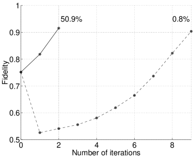
FIG. 3.: Fidelity as a function of the number of iterations for the optimized scheme (solid line) and for the QPA (dashed line) with the initial state given by Eq. (25). Joint probabilities of obtaining the required states are indicated.

A Cases when the QPA is inefficient

As the first example, consider the state

$$\varrho_{1}=\varrho_{2}={\textstyle\frac{20}{33}}|\gamma\rangle\langle\gamma|+{\textstyle\frac{5}{33}}|\psi^{-}\rangle\langle\psi^{-}|+{\textstyle\frac{8}{33}\frac{1}{4}}I,$$ (25)

where $|\gamma\rangle$ = $2^{-1/2}(0,1,i,0)^{{\dagger}}$ and $I$ is the 4$\times$4 identity operator. The overlap of this state with the Bell state $|\psi^{-}\rangle$ is $17/33$ $\approx$ $0.5152$, which is marginally sufficient for using the QPA algorithm, and the fidelity defined above is $F$ = 0.7518. Let us assume that the aim is to exceed $F$ = 0.9, which may be sufficient for application of other distillation schemes, e.g., the hashing method [2]. A direct application of the QPA method would reach this value after 9 steps, the joint probability of success in all steps being 0.81% (see Fig. 3). This would require an average number of 63$\times 10^{3}$ pairs to get a single output pair. On the other hand, our optimization scheme would reach the required fidelity in 2 steps with a joint probability of 50.87%, so that less than 8 pairs on average are consumed to get one output pair, which clearly means a substantial improvement of distillation efficiency [15].

B Application to states with fidelity $<$ 1/2

If the entangled pairs have fidelity $F$ $<$ 1/2, one cannot directly use the existing methods [1, 3] to distill the entanglement. So far, the only suggested scheme to handle such pairs would be to transform them first by non-unitary operations such as filtering [5], in order to reach fidelity above 1/2. To our knowledge, no explicit formula for determining the filtering parameters for arbitrary states has been presented.

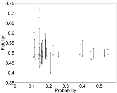
FIG. 4.: Purification of inseparable states with $F$ $<$ 1/2. The vertical coordinate of the circle of each arrow denotes the fidelity of the initial state, whereas that of its tip corresponds to the fidelity of the resulting state after one step of optimized distillation. The horizontal coordinate of each arrow indicates the probability of success of the distillation procedure. The Figure shows 25 examples of the optimized distillation procedure for randomly generated initial states.

Our approach allows for entanglement distillation of pairs with $F$ $<$ 1/2 in the same way as for any other entangled states. To demonstrate this, we have randomly generated several density matrices with $E$ $>$ 0 and $F$ $<$ 1/2, and optimized the local unitary transformations so as to reach a state with $F$ $>$ 1/2 (see Fig.4). We have observed that, whereas the success of the optimization depends on the value of $E$ in the initial state, it still works for all randomly generated states with entanglement above 5$\times 10^{-4}$, allowing inseparable states with $F$ $<$ 1/2 to be purified using only unitary transformations and conditional measurements, without filters. Notice that starting from a fixed value of $F$, the distillation can exhibit either a large increase of $F$ with a small probability or vice versa [15].

C Application to trapped ion qubits

Significant improvement in distillation efficiency is achieved by our method not just for rather special, but also for generic, physically important cases. For instance, let us consider qubits that are realized by two internal states of trapped ions [16]. If two or more ions are trapped in a single trap, then the logical functions between two qubits are achieved by using an auxiliary internal state of each ion and a vibrational mode of the collective oscillations. It is assumed that the evolution of the ionic states is driven by coherent laser pulses whose amplitudes, phases and durations can be controlled. An arbitrary unitary transformation of a single qubit can be achieved by two resonant laser pulses focused on the corresponding ion [16]. The durations (or strengths) of the two pulses and the phase of (say) the second pulse represent 3 parameters of the transformation. The interaction between two ions is achieved by a sequence of three pulses, whose effect is to flip the sign of the state $(0,0,0,1)^{{\dagger}}$ (i.e., $|e_{1},e_{2}\rangle$) without changing the other basis states. The parameters of these three pulses are fixed at properly chosen values so as to ensure that at the end of the procedure no auxiliary state remains excited (see [16] for details).

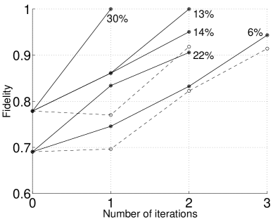
FIG. 5.: Fidelity as a function of the number of iterations for the optimized scheme (solid lines) and for the QPA scheme (dashed lines). Entanglement distillation for two different initial states is repeated until the fidelity $F$ $=$ 0.9 is reached. The upper tree (starting with $F$ = 0.779) corresponds to a decayed singlet (after a decay time $\gamma t$ $=$ 0.25) as the initial state. The lower tree (starting with $F$ = 0.691) corresponds to the same decayed singlet mixed with a completely mixed state as the initial state. Joint probabilities of obtaining the required states are indicated for the optimized scheme.

Let us call this transformation $U_{c}$, and assume that during one step of distillation each party performs only one transformation $U_{c}$, preceded and followed by single-qubit rotations. Rotation of all 4 qubits before the $U_{c}$ transformation represents 4 $\times$ 3 = 12 parameters. After the $U_{c}$ transformation it is sufficient to rotate only the two qubits which are to be measured, as the local transformations of the remaining pair do not change the entanglement. Thus, we are left with 12 $+$ 2 $\times$ 3 = 18 parameters to be optimized, their physical meaning being the areas and phases of the laser pulses.

As an example of entanglement decoherence, let us take the ionic excitation to be decaying according to the (zero-temperature) master equation

$$\dot{\varrho}=-{\textstyle\frac{i}{\hbar}}\left[H,\varrho\right]-{\textstyle\frac{\gamma}{2}}\left(\sigma_{+}\sigma_{-}\varrho+\varrho\sigma_{+}\sigma_{-}\right)+\gamma\sigma_{-}\varrho\sigma_{+}.$$ (26)

Here the (single-particle) Hamiltonian is $H$ $=$ $\hbar\omega_{0}$ $|e\rangle\langle e|$, with $\sigma_{+}$ $=$ $|e\rangle\langle g|$ and $\sigma_{-}$ $=$ $|g\rangle\langle e|$, where $|g\rangle$ and $|e\rangle$ denote the ground and the excited states, respectively. The upper “tree” in Fig. 5 has as its starting point the state obtained by the decay of the singlet $|\psi^{-}\rangle$ according to Eq. (26), after a decay time $\gamma t$ = 0.25. This state has fidelity $F$ = 0.779. Again, we can assume that the aim is to purify the state so as to reach fidelity of at least 0.9. The QPA procedure would achieve this goal in 2 steps, consuming on average 7.7 pairs and ending up with a state whose fidelity is $F$ = 0.918. Using the optimization scheme with 18 parameters, the pairs have a relatively large probability to be fully entangled ($F$ $=$ 1.0) after the first or second step. We are able to reach full entanglement in this case because the decayed singlet has zero probability for both qubits to be in the excited state, as opposed to a Werner state. Following the different trajectories of our procedure, we find that the mean number of pairs consumed before reaching $F$ $=$ 0.9 is only 4.6.

The lower tree in Fig. 5 starts from a state obtained by mixing the decayed singlet after $\gamma t$ $=$ 0.25 with a fully mixed state in a 83% to 17% proportion, as a result of additional sources of errors. In this case, even the optimization scheme yields only partially entangled states. However, whereas the QPA procedure would need 25.8 pairs on average to get the required fidelity, the optimization scheme would consume only 15.8 pairs on average for this task [15].

IV Discussion

Our main achievements can be characterized as finding a straightforward method for efficient distillation of entanglement, which is particularly valuable in cases where previously suggested methods either do not work or converge relatively slowly. There is no special requirement on the form of the initial states (such as the Werner states), except that the states must be entangled. It is not even required that the fidelity should be larger than $1/2$. We have seen that this approach allows essential saving of the “raw material” of initial partly entangled states.

Several points must be noted: (i) The optimization procedure may end in a local extremum of the cost function, which usually requires several trials before the final choice of the transformation parameters. (ii) By contrast to the previous schemes [1, 3], our method is state-dependent: before starting the distillation we have to know the initial density matrix. This knowledge is consistent with the objective of protecting particular correlated two-qubit states, e.g., singlets, from being spoilt. The knowledge of the initially spoilt state can be achieved either by familiarity with the dissipation or error dynamics (e.g., zero-temperature decay - Sec. III C), or by state reconstruction methods (the problem of density matrix reconstruction by local measurements of a pair of two-level systems has been studied in detail in Ref. [17]). Of course, in the latter case a portion of the pairs will be consumed for the reconstruction measurements, but once the density matrix is determined with sufficient precision, the distillation scheme can run indefinitely. Note that the knowledge of the density matrix would be necessary also in the case of the QPA method when $F$ $>$ $1/2$ but no diagonal density matrix element in the Bell representation is larger than $1/2$: the state must be properly rotated before the QPA method itself is used, and the parameters of the rotation would depend on the initial state.

REFERENCES

- [1] C.H. Bennett, G. Brassard, S. Popescu, B. Schumacher, J.A. Smolin, and W.K. Wootters, Phys. Rev. Lett. 76, 722 (1996).
- [2] C.H. Bennett, D.P. DiVincenzo, J.A. Smolin, and W.K. Wootters, Phys. Rev. A 54, 3824 (1996).
- [3] D. Deutsch, A. Ekert, R. Jozsa, C. Macchiavello, S. Popescu and A. Sanpera, Phys. Rev. Lett. 77, 2818 (1996).
- [4] C. Macchiavello, Phys. Lett. A 246, 385 (1998).
- [5] M. Horodecki, P. Horodecki and R. Horodecki, e-print quant-ph/9607009 (1996); see also N. Gisin, Phys. Lett. A 210, 151 (1996).
- [6] C.H. Bennett, G. Brassard, C. Crepau, R. Jozsa, A. Peres, and W.K. Wootters, Phys. Rev. Lett. 70, 1895 (1993). For recent experimental results see D. Bouwmeester, J.W. Pan, K. Mattle, M. Eibl, H. Weinfurter, and A. Zeilinger, Nature 390, 575 (1997); M.A. Nielsen, E. Knill, and R. Laflamme, Nature 396, 52 (1998); D. Boschi, S. Branca, F. De Martini, L. Hardy, S. Popescu, Phys. Rev. Lett. 80, 1121 (1998); A. Furusawa, J.L. Sorensen, S.L. Braunstein, C.A. Fuchs, H.J. Kimble, and E.S. Polzik, Science 282, 706 (1998).
- [7] A. Ekert, Phys. Rev. Lett. 67, 661 (1991). For recent experiments see W.T. Buttler, R.J. Hughes, P.G. Kwiat, S.K. Lamoreaux, G.G. Luther, G.L. Morgan, J.E. Nordholt, C.G. Peterson, C.M. Simmons, Phys. Rev. Lett. 81, 3283 (1998); W. Tittel, J. Brendel, H. Zbinden, and N. Gisin, Phys. Rev. Lett. 81, 3563 (1998).
- [8] K. Życzkowski, P. Horodecki, A. Sanpera and M. Lewenstein, Phys. Rev. A 58, 883 (1998).
- [9] Strictly speaking, the proportions may depend on what is chosen as the “uniform” distribution of the states, see discussion by P.B. Slater, e-print quant-ph/9809042 (1998).
- [10] G. Harel, G. Kurizki, J.K. McIver, and E. Coutsias, Phys. Rev. A 53, 4534 (1996); M. Fortunato, G. Harel, and G. Kurizki, Opt. Commun. 147, 71 (1998).
- [11] K. Życzkowski and M. Kuś, J. Phys. A 27, 4235 (1994).
- [12] An explicit formula for calculation of the entanglement of formation for qubit pairs has been found by S. Hill and W. Wootters, Phys. Rev. Lett. 78, 5022 (1997), see also W. Wootters, Phys. Rev. Lett. 80, 2245 (1998).
- [13] Other measures of entanglement have been suggested: V. Vedral, M.B. Plenio, M.A. Rippin, and P.L. Knight, Phys. Rev. Lett. 78, 2275 (1997); V. Vedral, and M.B. Plenio, Phys. Rev. A 57, 1619 (1998); M. Lewenstein and A. Sanpera, Phys. Rev. Lett. 80, 2261 (1998); G. Vidal and R. Tarrach, Phys. Rev. A 59, 141 (1999); D.P. DiVincenzo, C.A. Fuchs, H. Mabuchi, J.A. Smolin, A. Thapliyal, and A. Uhlmann, Proceedings of the 1st NASA International Conference on Quantum Computing and Quantum Communication, to be published, e-print quant-ph/9803033 (1998).
- [14] R.F. Werner, Phys. Rev. A 40, 4277 (1989).
-
[15]
More detailed data
can be found at the internet address
http://chemphys.weizmann.ac.il/~opatrny/seq2.txt. - [16] J.I. Cirac and P. Zoller, Phys. Rev. Lett. 74, 4091 (1995).
- [17] V. Bužek, G. Drobný, G. Adam, R. Derka, and P.L. Knight, J. Mod. Opt. 44, 2607 (1997); V. Bužek, G. Drobný, R. Derka, G. Adam, and H. Wiedemann, e-print quant-ph/9805020.