Operational Time of Arrival in Quantum Phase Space
Abstract
An operational time of arrival is introduced using a realistic position and momentum measurement scheme. The phase space measurement involves the dynamics of a quantum particle probed by a measuring device. For such a measurement an operational positive operator valued measure in phase space is introduced and investigated. In such an operational formalism a quantum mechanical time operator is constructed and analyzed. A phase space time and energy uncertainty relation is derived.
pacs:
PACS number(s): 03.65.Bz, 42.50.DvI Introduction
The problem of the proper definition of the quantum mechanical time observable, and the physical interpretation of the associated uncertainty relation between time and energy, is a subject of a long lasting debate. This is due to the fact, that both in classical and quantum nonrelativistic mechanics, the time parameter is not an independent dynamical variable, and its definition requires the use of a nonlinear function of the canonical variables describing the system. In classical physics the form of this nonlinear function does not bring any conceptual difficulties, for instance, for a free particle of a unit mass and in one dimension, with an initial momentum and an initial position , the time of arrival from to a fixed position is given by
| (1) |
In the general case of an arbitrary motion it is necessary to invert the equations of motion for a particle in order to find the time parameter . This function can be in general multivalued and the choice of the form is selected according to the physical meaning of the given solution.
In quantum mechanics the problem of the definition of the time observable associated with such a nonlinear transformation becomes much more complicated since canonical observables are noncommuting operators. This makes, for instance, the definition like (1) ambiguous due to the ordering problem of and operators.
It was Pauli, who first originated the question whether one can define a time operator as a canonical variable conjugated to the energy of the system. In his book on quantum mechanics [2], he pointed out, that although formally we can write , this formula is unsatisfactory since the operator cannot be Hermitian due to the semi – bounded character of the Hamiltonian spectrum. As a result, the uncertainty relation in the form has a disputable interpretation.
One can derive, however, the above uncertainty relation using a Fourier decomposition of a nonstationary state in the form . In such an approach, the uncertainty relation is a simple consequence of Fourier analysis, similar to the one encountered in classical Fourier optics for time-dependent fields and their spectra. A similar argument can be applied to derive the position and the momentum uncertainty relation of a wave packet in wave mechanics. However, it is well known that this last uncertainty relation has a much deeper meaning being the consequence of the fundamental quantum incomplementarity of two canonical variables – momentum and position. Such an approach to quantum nonstationary states was presented first by Fock and Krylov [3], and in the basically same spirit by Mandelstamm and Tamm [4]. In these works the relation between the energy of the system and its “inner” time [5], which usually is the lifetime of the nonstationary quantum state, has been derived and discussed
Another approach was proposed by Landau and Peierls [6] and by Fock and Krylov [3] who discussed the problem of the time-energy uncertainty relation analyzing a typical scattering experiment of a particle on a test particle. The essential conclusion of these contributions was that the uncertainty relation is connected with the inability of measuring precisely the energy of a given system in an arbitrary short period of time.
Neither of the above proposals lead to the definition of the time operator, what’s more, it has been shown by Aharonov and Bohm [5] that the interpretation given by Landau and Peierls is erroneous i.e., it is possible to measure the energy in a time period which violates the postulated uncertainty relation. In the same article Aharonov and Bohm proposed a different approach to the problem of the time observable. They argued that in order to measure the time of arrival to a certain fixed point one needs to have a “quantum clock” i.e., another quantum system, which reads the experimental data collected during a clock measurement. This assumption led to the first explicit definition of the time observable in the form proposed by Aharonov and Bohm:
| (2) |
where are the operators of the clock particle. This definition formally leads to the commutation relation , where is the Hamiltonian of a clock particle. However such a time operator has an important disadvantage, in an a priori imposed and physically unjustified choice of a symmetric ordering of momentum and position operators. On the other hand, such an operator has a number of interesting properties [7, 8] that indicate possible physical applications.
This fact can be understood in two ways.. First, it has been shown in Ref. [9, 10], that with the Aharonov – Bohm time operator (2) one can associate a positive operator valued measure (POVM), or equivalently, a realistic measurement scheme, whose outcomes are described by such an observable.
Another interpretation of the Aharonov – Bohm formula (2) might be given in the framework of the approach proposed by Kijowski [11]. It was shown there, that by a construction of a probability distribution for a particle to pass at a certain moment a two dimensional reference plane, one can define a time operator. The explicit formula for such a time operator is like (2):
| (3) |
where the multiplicative sign of the momentum operator assures the Hermitian character of the time observable [12]. Physically, the sign function means that one distinguishes between particles moving to the left and to the right with respect to chosen two dimensional reference plane. For an initial beam of particles prepared in such a way, that it contains only particles moving either to the left or to the right, the time operator (3) reduces to the original Aharonov and Bohm formula (2). One should however note that this time operator is built from the operators describing the measured particle, and not from some clock particle operators like in the Aharonov – Bohm approach.
The time operator (3) is conjugated to the variable , and as a consequence leads to a corresponding uncertainty relation [11, 12].
It has been shown in [13, 14] that one can use the above definition as a starting point to look for a time observable. The definitions of the time observable given by Kijowski [11, 12] and by Delgado and Muga [13, 14] are then equivalent.
It shall also be stressed, that contrary to the claims of some authors [7, 13], the time operator (3) is defined in the framework of standard quantum mechanics, although in a rather unusual representation of the wave function, which is, however, as good as any other representation (see comment [12]).
It is also worth noticing that a symmetrized operator like (2) is naturally connected with a probability distribution of arrival times derived from an expectation value of the properly defined positive current operator [13, 14].
After a number of early, classical papers, which stated the problem and revealed the main difficulties in dealing with the question of the time observable in quantum mechanics, there was a large number of further works. Although our brief review of the published literature is far from being complete, we would like briefly to describe several approaches in order to place our own work in some historical and logical context. An excellent study, of both older and newest researches connected with the problem of time observable in quantum mechanics, can be found in [15].
Roughly speaking, the majority of the research efforts in this field can be divided into the following three approaches.
In the first approach the main effort was concentrated on the proper definition and understanding of various time and energy uncertainty relations. In such relations, the meaning of both time and energy, varied depending on the author and the presented method. The most complete, known to us, review of this problem can be found in Ref. [16]. Newest investigations on this issue have been presented in Ref. [17].
Another way of dealing with the time observable was to define a time operator as a symmetrized function of the position and momentum operators [7, 8]. This approach was discussed above and is justified by the work of Kijowski.
The third method, the closest to our proposal, is based on the investigation of a particle, whose time of arrival to a given point is detected by a certain reference “quantum clock”. This quantum clock is represented by another quantum system, which has some properties enabling us to read the time of arrival of the measured particle. Obviously, one can design many different models of such quantum clocks. Depending how one chooses the system representing the quantum clock, and how one models the interaction between the clock and the investigated particle different nonequivalent schemes of time measurement can be introduced. Examples of various “quantum clocks” can be found in [9, 17, 18, 19].
Another interesting discussion of the realistic, irreversible, detector model has been presented by Halliwell [20]. The decoherent histories approach to the arrival time problem has been given by the same author in Ref. [21]. In this paper a probability distribution to find a particle in a certain position in a given fixed time interval has been introduced,
using similar idea presented earlier by Yamada and Takagi [22].
This has to be contrasted with the standard quantum approach, when such a probability is introduced only for a given moment of time. A similar approach, in which the detector is not specified as another quantum system, but rather is treated phenomenologically without explicit treatment of the interaction of the measured system and the experimental device, is given in Ref. [23].
One can also ask, if it is possible to choose among the different quantum clocks those which are the most precise, in a sense that they saturate the time – energy uncertainty relation. This question has been addressed in Ref. [24].
A very extensive and general analysis of various aspects of the proper treatment of the time observable has been given in the papers by Allcock [25] and by Mielnik [26].
It is the purpose of this paper to define an arrival time operator based on a realistic momentum and position measurement. Our work is mainly motivated by a recent successful experimental approach, in which operational measurements of the quantum phase of optical fields have been performed [27]. Such operational measurements have been related to simultaneous joint measurements of position and momentum operators in a space extended by the measuring device.
In this paper we define an operational time operator, which is connected with a very simple model of a joint momentum and position measurement. Such a measurement may be implemented [28, 29, 30, 31], if additional degrees of freedom responsible for the measuring devices are involved. For such a measurement we introduce the operational time observable and a corresponding POVM. We show that for a special case of the quantum clock state, the arrival time operator involves an antinormal ordering of the creation and annihilation operators forming the canonical variables. The operational phase space measurement leads to a time and energy phase space. For such a phase space and for an operational time of arrival a time and energy uncertainty relation is derived.
This paper is organized in the following way. A short review of the general operational approach will be discussed in Section II. In Section III we present a quantum model for a joint measurement of position and momentum in a space extended by the measuring device. This allows to construct a corresponding POVM relevant to the definition of the operational time observable. From this POVM a positively defined operational probability distribution function called propensity is derived. This propensity leads to a mean time of arrival. In Section IV we introduce an explicit form of the operational time of arrival. We derive the time operator and show that the specific ordering of the position and momentum operators, forming this observable, depends on the properties of the measuring device. Using the time operator, constructed in such a way, we derive in Section V an operational time and energy uncertainty principle. In Section VI we introduce a time and energy phase space. We show that an arrival time distribution can be interpreted in terms of a positive and negative flux flow. Finally Section VII contains some concluding remarks.
Through the rest of the paper we shall work in one dimension and use the units in which , .
II Operational Quantum Measurement
A Operational POVM
In order to describe realistic experiments involving measuring devices it is sometimes necessary to go beyond the idealized measurement scheme proposed by von Neumann [32]. In this approach it is postulated, that statistical outcomes of a measurement of a certain observable with eigenvalues and eigenvectors are described by the spectral measure:
| (4) |
where is the state vector of the measured system. It is known that the spectral measure contains all the relevant statistical informations about the investigated system but it makes no reference to the apparatus employed in the actual measurement. Due to this property will be called an intrinsic quantum observable. In order to provide a more realistic approach to the quantum measurement we need to analyze carefully the dynamics of the combined system involving both the measured system and the measuring apparatus. We shall call for short the measuring apparatus and all its associated devices a filter device. Such an approach has been presented by many authors [28, 29, 30, 31] and we shall use here the formulation and notation from [28, 29].
Let the state of the measured system be described by the density operator in a Hilbert space and the state of filter device by in a Hilbert space . The evolution of the combined system, including the interaction between the filter and the investigated system necessary for the measurement to happen, is given by a unitary operator acting in :
| (5) |
In order to probe the system state with such an interaction, the statistical readouts of the filter device are collected. The corresponding probability distribution corresponds to a propensity of the measured state to take on certain states of the filter. Due to the interaction the propensity of the probed state to be in one of the filter states is
| (6) |
where is a filter dependent POVM satisfying the normalization condition
| (7) |
B Operational operators
In view of the linear relation between the propensity and the POVM, the operational statistical moments of the measured quantity
| (8) |
define uniquely a set of operational operators
| (9) |
A real number is a classical quantity which enables us to read out the result of the quantum mechanical measurement. Since a real measurement operates in a classical world the outcomes of such an experiment are known only if they are macroscopically recorded [33]. This is why the result of such an experiment will be given by the probability distribution of a certain classical variable. In the presented approach this distribution is just the quantum propensity .
The operators (9) are called operational operators, because they represent quantities measured in a real experiment involving a dynamical coupling of the measured system with the filter. We see that in a realistic measurement, with a filter, the spectral decomposition of an observable is effectively replaced by a POVM [30]. As a rule, the algebraic properties of the set differ significantly from those of the powers of . For instance, . This property will have important consequences in the discussion of the uncertainty introduced by the measurement. As an example the operational spread of a measured quantity, described by the of operational operators, is given by
| (10) |
This relation will play an important role in the formulation of the operational uncertainty relation.
It is seen that the propensity and the operational operators are natural extension of the spectral probability distribution and the intrinsic operators. The difference is that the operational observables carry information about the system under investigation and the selected measuring device. There always exists a physical mechanism (a realizable experimental procedure) generating any desired POVM. This is guaranteed by the Naimark extension, and the reduction of the projection measure into the Hilbert space of the measured system [30]. According to this theorem one can always extend the Hilbert space with the defined POVM to a space with a projective measure.
III Joint Momentum and Position Measurement
A Joint measurements in phase space
In this section we present a simple model of a joint position and momentum measurement proposed originally by von Neumann [32] and elaborated later in Ref. [34, 35, 36].
The interaction Hamiltonian between the system (a particle) and two filter particles (labeled by and ) is given by
| (11) |
After the pulsed interaction with the system, the measured readouts and of the filter variables and are:
| (12) | |||||
| (13) |
In the combined space of the two filter particles, we introduce filter operators and . In the product space of the system and the filter the two measured observables (12) are:
| (14) |
We recognize in the relations (14) the position and the momentum observables of a composed system introduced and discussed first by Einstein, Podolsky and Rosen in their famous paper on the completeness of quantum mechanics [39].
In our case the filter particles provide an example of the Naimark extension of and . In the extended space, the filter readout variables commute:
| (15) |
and, as a result, can be measured simultaneously. From this definition, we can introduce in this extended space a time observable:
| (16) |
where the ordering of the commuting measured observables is irrelevant. This expression will be central in the following investigations. The reduction of this operator to the Hilbert space of the measured particle will provide an operational definition of the time of arrival in phase space. As an example we obtain in the space of the particle the following operator:
| (17) |
Using the definition of the propensity (6) from Section II (with being and ), and the above interaction Hamiltonian we obtain that the propensity is a phase space distribution:
| (18) |
where and are the wave functions of the particle and the filter in the position representation labeled by . In fact the filter wave function is an overlap of the wave functions of the two particles and forming the measuring device. The POVM in the Hilbert space of the system that corresponds to this measurement scheme is
| (19) |
B Mean time of arrival
We shall apply this measurement to probe the time of arrival of a freely moving particle probed by a filter device. In this case the mean time of arrival will be simply related to the mean relative position of the measured particle with respect to a fixed filter position. In order to describe such a measurement we shall apply the derived above phase space distribution.
In such a case the propensity becomes time dependent via the wave function of the measured system. In order to carry all the calculations in an analytic form, we shall assume that the time measurement is performed on a freely moving particle described by the following Gaussian wave function:
| (20) |
characterized by the initial mean position , the initial mean momentum and width . The filter wave function, at the measurement time , is assumed to be in a stationary state with a Gaussian profile centered around with width
| (21) |
As it is seen, due to the pulsed interaction between the filter and the particle, the dynamics of the filter particle is unimportant.
For this choice of the two wave packets the time evolution of the propensity is easily calculated
| (23) | |||||
To understand the meaning of the propensity associated with this measurement we calculate its first two phase space moments
| (25) |
| (26) |
| (27) |
| (28) |
We see, for instance, that the average gives the relative position of a particle measured with respect to the filter position. This fact reflects the fundamental property of the measurement in which the arrival time to a fixed position is monitored by a filter device.
The cross section of the propensity in for a fixed value of , as a function of is depicted on Fig. 1. In this case the particle moves from a point towards the detection point of the filter. Note a full symmetry between positive and negative values of , around the measurement time set at . With the passage of time, the distance between the measured particle and the filter particle is shrinking, and finally it is zero, meaning that the measurement corresponding to the arrival time at the point has been performed. Due to the unavoidable dispersions of the particle and the filter wave packets the propensity is spreading in time, deteriorating the measurement precision. The accuracy of such a measurement might be improved in several ways. We can use well prepared wave packets of the system i.e., wave packets with a small dispersion, or we may prepare the filter state in a squeezed state [37], with a reduced position dispersion. The measured momentum is constant in time, which is a unique feature of the Hamiltonian with a pulsed (Dirac delta function) interaction in time.
IV Time Observable
A Operational time of arrival
From the phase space propensity derived in the previous section it is straightforward to define a mean arrival time and its moments using the following definition:
| (29) |
where the integration region is the whole phase space. According to the general relation between the moments (8) and the operational operators (9), we introduce a family of operational time operators:
| (30) |
where in terms of the operational time POVM (19):
| (31) |
We notice immediately that for our choice of the propensity the -integral is divergent due to a singularity at . This singularity can be easily understood on the physical ground, related to the concept of the arrival time discussed above. The physical reason for the singularity is that the particle with zero momentum will never arrive to the measurement point, implying an infinite arrival time.
Obviously if we change the measurement scheme in such a way that (introducing for example a proper external potential) the particle is forced to move towards the detection point, the infinity in (31) would be removed. In fact such a divergence is not unusual in quantum mechanics, when for instance, vectors of the Hilbert space corresponding to an infinite mean value of the position operator are used. For the time operator operationally based on the measurement of the arrival time, we shall select only such states for which the probability of finding the particle with zero momentum is very small.
In order to remove the divergence we can apply a regularization procedure, removing from the integration region the values of near zero. As a result we obtain:
| (32) |
where for . A similar regularization for a differently ordered time operator was described in great detail in Ref. [7]. Our conclusion is analogous to the results of this paper. If the initial wave packet is prepared in such a way that it has a vanishing distribution of momentum near , the final results involving the time operator are independent of the regularization procedure. The condition which must be fulfilled is that .
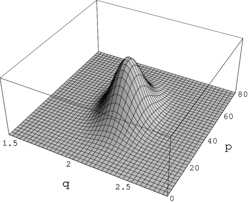
On Fig. 2 we have depicted the phase space propensity for a selected set of values of and . From this plot of the propensity, we see that it is enough to set, for example, and (in our units) to have a propensity practically equal to zero in the required region. It is clear that if both the particle wave function and the filter wave function are badly localized, the notion of the time of arrival looses its meaning. In this case a different time operator ought to be introduced.
Because the only significant contribution in the phase space integration comes from the momenta concentrated around we can expand in (32) in the series around , (from a mathematical point of view such an expansion of the integrand will lead usually, after integration, to an asymptotic series). This greatly simplifies the integration in (32), and as a result we obtain the following leading contributions to the two first moments:
| (34) |
| (35) |
As we see, the leading contribution reproduces the semiclassical approximation of the motion of the particle. The physical interpretation of the obtained results is clear. The mean of, the introduced time operator, gives the time of flight between the two points and . This time of arrival is given as a ratio of the distance between two points and the particle momentum. Obviously there are quantum corrections to the formulas (IV A). These corrections are much more pronounced when a second moment of the time operator is investigated.
B Ordering and time of arrival
We shall derive now a more direct formula for the operational time operator (31) in the case of a particular choice of the filter wave packet parameters. We express the position and the momentum operators, in terms of the oscillator creation and annihilation operators, using the standard relations and . We set the filter wave function to be a state corresponding to . Such a state is a Gaussian wave function with dispersion in our units). Using this filter state and these operators we can rewrite the POVM as follows
| (36) |
where is the Glauber displacement operator in the complex phase space [38]. In such case, i.e., for such a filter wave function, the propensity is simply . We recognize in this expression the so called –representation used in quantum optics applications. It is well known that this function is related to the antinormal ordering of the creation and annihilation operators ( to the right and to the left) [38].
The time observables then take a very simple form
| (37) |
where the triple dots denote the antinormal order of the creation and annihilation operators.
We see that the measurement scheme with this particular choice of the filter wavepacket leads naturally to an antinormal ordering of the creation and annihilation operators, which reflects a specific ordering of the momentum and position operators forming the operational arrival time observables (37). For a different choice of the width parameter , we will have a different ordering of these operators (see [35] for details).
As it was discussed above, only these states, which have vanishing amplitudes for momenta equal to zero are physically interesting, and for such states the time operator written above is well defined. Such states specify the domain of the operator (37).
In that spirit we will find a more explicit formula for the first two moments of the time operator. We need to express the inverse of antinormally ordered (in the discussed above sense) momentum operator as a direct function of momentum operator centered around :
| (38) |
In this formula will be understood as mean value of momentum of a detected particle, and that states with zero momentum are excluded. Naturally, the above equality holds only when we assure that there is a domain of vectors }. All the following formulas will have a physical meaning for states belonging to the this domain.
In the next derivations we shall use the following algebraic identity:
| (39) |
where is an arbitrary parameter. Using this formula simple algebra gives
| (40) |
where are Hermite polynomials. In order to find a second moment of a time operator we need the following expression
| (41) |
All higher powers are easily obtained by the subsequent derivation over , and then taking the limit , as shown above for .
Combining these algebraic properties we obtain the following formulas for the first two moments of the operational time operator:
| (42) | |||||
| (43) |
where was calculated above.
In the subspace an arbitrary moment of the operational time operator can be written in the following form:
| (44) |
where the subscript index is of order , and a systematic method of calculating all follows from the algebra presented above. For sufficiently large values of i.e., for a fast moving particle we can well approximate the formula for the time operator by the first few terms in the series. For we have:
| (45) |
where
| (47) |
| (48) |
| (49) |
The zero order term reproduces the classical limit corresponding to an arrival time of a particle with momentum at a fixed position .
For we have
| (51) |
| (52) |
Even in the zero order approximation the second moment of the time observable does not reproduce the classical limit, in particular we see that .
Usually when we deal only with mean values of observables, the difference between results obtained with the help of an intrinsic operator (if such exists) and the operational operator is rather simple and straightforward. The first moment of the operational operator equals to the intrinsic operator, or differs by a term simply connected to the properties of the of the filter device. The situation becomes quite different for the second moments. In the operational formalism the second moment contains a contribution representing quantum fluctuations of the filter. Due to the additive character of the presented measurement the time operator contains an additive quantum noise contribution from the filter system.
We conclude this section investigating the eigenfunctions of the time operator. The eigenvalue problem for the operational time of arrival has the following form:
| (53) |
In the following we derive the eigenvectors for several approximated values of . In the zero approximation, for , the eigenstate can be simply calculated in the momentum representation. For a given eigenvalue this eigenvector is just
| (54) |
where we have introduced a new variable . As it is seen, the eigenstates are labelled by the momentum of the inspected particle. If we treat as a physical time, we can write , and then can be interpreted as the time of flight from the point to a fixed point . The spectrum of this operator is continuous.
The eigenfunctions of the time operator involving the higher order contribution can be obtained solving a first order differential equation. As a result we obtain:
| (55) |
This eigenfunction will belong to the domain , if . The connection with the eigenfunction in the lower order of approximation and the interpretation of this result is best seen upon expanding the eigenfunction in powers of the parameter , we have then
| (56) |
where, as above, . From this expression we conclude that the phase of this eigenfunction is the classical arrival time with nonclassical contributions resulting from the higher order term .
V Operational time-energy uncertainty
In the approach presented in this paper it is easy to give a clear meaning to the time and energy uncertainty relation. This is because that, on the operational level, we can describe a measurement of both the time of arrival for a given system and its energy. The operational time operator is given by Eq. (31), and the corresponding operational moments of energy of the system are:
| (57) |
where is the momentum marginal of the phase space POVM (19). It should be pointed out that the defined below uncertainty relation is given between the measured time of arrival and the measured energy of the chosen system, and as a result, the criticism of Aharonov and Bohm [5] and Peres [31] concerning those approaches where one tried to construct the uncertainty principle between the time of arrival detected by the filter and the energy of the investigated particle (two commuting quantities) does not apply here.
Using the general formula for the operational spread introduced in Section II, we introduce the operational spread of the time operator
| (58) |
This quantity can be calculated using Eq.(35). The corresponding operational spread of the energy is:
| (59) |
The mean operational energy has been already calculated (28) and we need only
| (60) |
Simple algebra gives,as a result, an operational time-energy uncertainty in the form:
| (61) |
When both and are approaching simultaneously zero, the right hand side of the above inequality tends to (i.e., ), meaning that the “conventional” uncertainty relation is reproduced if the particle and filter states are very well prepared. However, we have to remember that these calculations have been performed under the assumptions that and . This corresponds to the position spread of the wavepackets very small and hence giving the momentum spread very large.
We conclude this section calculating the commutator involving the energy and the operational time operator derived for a filter state leading to an antinormal form. As it was said before, these first moments of the operational operators should in some sense be the closest to the intrinsic time and energy observables. A simple algebra shows that:
| (62) |
The right hand side of this commutator is complicated, but for states belonging to the domain we obtain that the leading term is:
| (63) |
Only in this limit, one can associate the traditional interpretation of and as canonically conjugated variables for time and energy.
VI Time and Energy Phase Space
A Probability distribution of time of arrival
The definition of the operational time of arrival operator is related to the following moments of the corresponding phase space propensity. It seems natural then to introduce a differently parameterized propensity i.e., instead of working with as a function of , we shall define a new arrival “time” variable (to be not confused with the time labelling the evolution of the system wave function):
| (64) |
From the properties of the Dirac delta function we obtain
| (65) |
The interpretation of this result is simple in terms of the right and left operational probability flux.
This result should be contrasted with the standard quantum current operator
| (66) |
The expectation value of this current seems to be a natural and intuitive candidate for the probability distribution of the time of arrival at the given space point . It is however difficult to make a practical use of this intuition since the flux (66) is nonpositive and it is difficult to associate with such a nonpositive flux a probability distribution. A discussion of this problem has been presented by Delgado [14].
Because the position and the momentum of the particle cannot be specified with arbitrary precision there is a possibility for a quantum backflow contribution to , if it is understood as a probability distribution. As it was pointed out in Ref. [14], when this backflow part of the probability distribution becomes negligible one can use this formula to define the time observable. Indeed, if a wavepacket is constructed in such way that the mean value of the momentum is positive and large, and a small negative part of the flux can be neglected, the probability distribution for an arrival time is approximately positive. However, this backflow contribution is interesting in itself [23] since it is of purely quantum mechanical origin. This is why it is tempting not to exclude it from the flux considerations, and in our approach based on the operational propensity, there is no need to do so.
Contrary to the quantum mechanical flux (66), the operational flux given by (65) is clearly positive. And as we have seen in the previous sections an association between this flux and the time observable is very natural and simple. In fact the flux (65) is exactly the corresponding time of arrival probability distribution,
| (67) |
Obviously, in our approach we deal with the two parts of the flux. The “positive” part corresponds to the particle moving in the direction given by the mean value of the momentum . The “negative” (or backflow) part has obviously the opposite meaning. The presence of these two parts in the flux is clearly a purely quantum feature, because in the classical world the particle moves either to one or to the other direction with probability one. For our choice of the wavepackets the negative and the positive parts of the propensity (65) might be written explicitly:
| (69) | |||||
where
| (70) | |||||
| (71) | |||||
| (72) |
and is the error function. When the mean momentum is large and positive the contribution of the negative flux becomes small. In this case the ratio of these two parts might me approximated as follows:
| (73) |
When the particle is moving fast, , then becomes large and the above ratio tends to zero. Finally, the formula for the complete flux is given by
| (75) | |||||
This quantity is depicted on Fig. 3 for a particular choice of the wave function parameters. As it’s seen the backflow part of the flux is much smaller then the dominating “positive” part. What is important is the fact that in our considerations we do not have to neglect the “negative” momenta contribution. In fact our model measurement scheme allows to measure this part of the probability distribution.
It is also interesting to note, that having defined the time observable Delgado and Muga [13, 14], also have managed to associate with it a positively defined current. This shows that such a relation is quite universal.
In analogy to the time distribution, we can define a complementary quantity, a probability distribution connected with the energy measurement:
| (76) |
Due to the pulsed interaction of the filter with the system, this distribution is time independent. Indeed, a simple calculation shows that:
| (77) |
B Time and energy phase space
In conclusion of this section we shall introduce a combined time and energy phase space for the operational measurement. In such a phase space we have a joint energy and momentum distribution defined as:
| (78) |
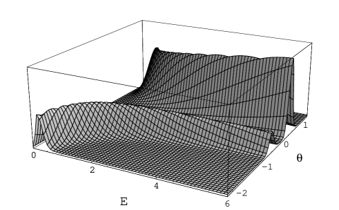
The time distribution (65) and the energy distribution (76) are marginals of this joint time and energy distribution. For the Gaussian wave functions we calculate
| (80) | |||||
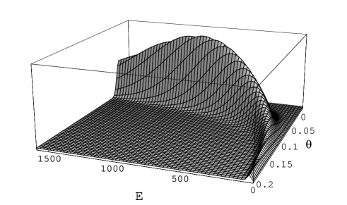
The meaning of this quantity becomes clear, when we look on its plot depicted on Fig. 4. We see the characteristic separation into two parts, one corresponding to the positive momenta (relative to ) and a much smaller contribution from the negative part. Further, we notice that for small values of energy the propensity is narrow in the direction but rather broad in the direction. This shows that the time measurement looses its meaning for very slow particles (small ). The situation changes in a complementary way when the energy is increased. This is depicted on Fig. 5, where the propensity becomes very sharp in the direction. This assures a sharp measurement of the time of arrival. In this case the energy measurement becomes less accurate.
The fact, that we have these two limits of the propensity is of course a manifestation of the time-energy uncertainty principle.
VII Conclusions
With the help of the operational formulation we have introduced an operational time observable associated with a specific measurement scheme. Such an operational approach is not universal, in a sense, that the specific form of the time observable depends on the quantum state of the filter device. This operational approach allows for a natural and clear definition of the time of arrival. Our result is an intuitive quantum counterpart of the classical time of flight measurement between two points. Based on such an operational approach the time – energy uncertainty principle has been introduced. The idealized measurement scheme allows to provide a link between the quantum mechanical flux of the operational propensity and the time observable. This has been done without neglecting the backflow part, which is very interesting.
The time operator discussed in this paper is related to a specific measuring scheme. The question remains what have we learned about the intrinsic time operator from our discussion. Our view is that various fundamental time operators will have many features of the operator . In fact we have shown that in terms of the commutation relations, classical limit and the physical interpretation, this operator has many features of an intrinsic time observable. However the problem is that we cannot provide a first principle derivation of this observable from some fundamental assumptions. The operational observable has been build using a specific detection procedure, but its overall properties should describe a intrinsic time operator in a reasonable way.
Acknowledgments
It is pleasure for us to acknowledge numerous discussions with Professor Jerzy Kijowski. This work has been partially supported by the Polish KBN grant No. 2 PO3B 118 12.
REFERENCES
- [1] Also at the Center of Advanced Studies and Department of Physics, University of New Mexico, Albuquerque NM 87131, USA.
- [2] W. Pauli, Handbuch der Physik, Vol. 5, Part. 1 : Prinzipen der Quantentheorie I, 1958.
- [3] V. Fock and N. Krylov, J. Phys. (U.S.S.R.) 11, 112 (1947).
- [4] L. Mandelstamm and I. Tamm, J. Phys. (U.S.S.R.) 9, 249 (1945).
- [5] Y. Aharonov and D. Bohm, Phys. Rev. 122, 1649 (1961); 134, B1417 (1964).
- [6] L. Landau and R. Peierls, Z. Physic 69, 56 (1931).
- [7] N. Grot, C. Rovelli and R. T. Tate, Phys. Rev. A 54, 4676 (1996).
- [8] J. G. Muga, C. R. Leavens and J. P. Palao Los Alamos preprint No. quant-ph/9807066.
- [9] P. Busch, M. Grabowski, P.J. Lahti, Phys. Lett. A 191, 357 (1994).
- [10] R. Giannitrapani, Int. J. Theor. Phys. 36, 1601 (1997).
- [11] J. Kijowski, Rep. Math. Phys. 6, 360 (1974).
- [12] J. Kijowski, Phys. Rev. A, to be published (1998).
- [13] V. Delgado and J. G. Muga, Phys. Rev. A. 56, 3425 (1997);
- [14] V. Delgado, Phys. Rev. A 57, 762 (1998); Los Alamos preprint No. quant-ph/9805058.
- [15] J. G. Muga, R. Sala, J. P. Palao Superlattices and Microstructures 23, 833 (1998) or Los Alamos preprint No. quant-ph/9801043.
- [16] M. Bauer and P.A. Mello, Ann. Phys. 111, 38 (1978).
- [17] Y. Aharonov, J. Oppenheim, S. Popescu, B. Reznik and W.G. Unruh, Phys. Rev. A 57, 4130 (1998); J. Oppenheim, B. Reznik and W. G. Unruh, Los Alamos preprint No. quant-ph/9807058 and quant-ph/9801034..
- [18] A. Peres, Am. J. Phys. 48, 552 (1980).
- [19] Y. Aharonov and J.L. Safko Ann. Phys. 91, 279 (1975).
- [20] J. J. Halliwell, Submitted to Phys. Rev. A; Los Alamos preprint No. quant-ph/9805057.
- [21] J. J. Halliwell, Phys.Rev. D 57, 3351 (1998).
- [22] N. Yamada and S. Takagi, Prog. Theor. Phys. 85, 985 (1991); 86, 599 (1991); 87, 77 (1992).
- [23] J. G. Muga, J. P. Palao and C. R. Leavens Los Alamos preprint No. quant-ph/9803087.
- [24] V. Buzek, R. Derka and S. Massar, Los Alamos preprint No. 9808042.
- [25] G. R. Allcock, Ann. Phys. (N.Y.) 53, 253 (1969); 53, 286 (1969); 53, 311 (1969).
- [26] B. Mielnik, Found. Phys. 24, 1113 (1994).
- [27] J. W. Noh, A. Fougéres and L. Mandel, Phys. Rev. A 45, 424; Phys. Rev. A 46, 2840 (1992) and references therein.
- [28] K. Wódkiewicz, Phys. Rev. Lett. 52, 1064 (1984); Phys. Lett. A 115, 304 (1986); Phys. Lett. A 124, 207 (1987).
- [29] B.–G. Englert and K. Wódkiewicz, Phys. Rev. A 51, R2661 (1995).
- [30] P. Busch, P.J. Lahti and P. Mittelstaedt, The Quantum Theory of Measurement (Springer–Verlag, Berlin 1991) and reference therein.
- [31] A. Peres, Quantum theory: concepts and methods (Kluwer, Dordrecht, 1993).
- [32] J. von Neumann, Mathematische Grundlagen der Quantenmechanik (Springer–Verlag, Berlin 1932).
- [33] N. G. Van Kampen, Physica A 153, 97 (1988).
- [34] E. Arthurs and J.L. Kelly, Jr., Bell. Syst. Tech. J. 44, 725 (1965).
- [35] S. Stenholm, Ann. Phys. 218, 233 (1992).
- [36] P. Kochański and K. Wódkiewicz, Rep. Math. Phys. 40, 245 (1997).
- [37] H.P. Yuen, Phys. Rev. A 13, 2226 (1976); for a review see: D.F. Walls, Nature 306, 141 (1983), R. Loudon and P.L. Knight, J. Mod. Opt. 34, 709 (1987), J. Opt. Soc. Am. B 4 (1987).
- [38] R.J. Glauber, Phys. Rev. 130, 2529 (1963);131, 2766 (1963).
- [39] A. Einstein, B. Podolsky and N. Rosen, Phys. Rev. 47, 777, (1935).
 |
 |
 |
 |
 |