Laser Field Induced Birefringence and Enhancement of Magneto-optical Rotation

Abstract

An initially isotropic medium, when subjected to either a magnetic field or a coherent field, can induce anisotropy in the medium and can cause the polarization of a probe field to rotate. Therefore the rotation of probe polarization, due to magnetic field alone, can be controlled efficiently with the use of a coherent control field. We demonstrate this enhancement of the magneto-optical rotation (MOR) of a linearly polarized light, by doing detailed calculations on a system with relevant transitions $j=0\leftrightarrow j=1\leftrightarrow j=0$.

I Introduction

An isotropic medium having $m$-degenerate sub-levels when subjected to a magnetic field exhibits birefringence in its response to a polarized optical field. This is due to the fact that Zeeman splitting of magnetic sub-levels causes asymmetry in refractive indices for left and right circular polarization components of the optical field. The result is magneto-optical rotation (MOR); i.e., the plane of polarization of the light emerging out of the medium is rotated with respect to that of the incident. If $\chi_{+}(\chi_{-})$ represents the susceptibility of the birefringent medium corresponding to right (left) circular polarization component of the probe, the rotation angle is given by

$$\theta=\pi k_{p}l(\chi_{-}-\chi_{+}),$$ (1)

where $\vec{k}_{p}$ corresponds to propagation vector of the probe and $l$ is length of the medium along the direction of propagation. The susceptibilities $\chi_{\pm}$ are functions of characteristics of atomic transitions and hence studies of $\theta$ yield information on atomic transitions. Extensive literature on MOR exists. Experiments have been carried out with both synchrotron and laser sources [1, 2, 3]. Effects of larger probe powers and resulting saturation have also been studied at length [4, 5, 6, 7].

The present study is motivated by the possibility that the susceptibilities $\chi_{\pm}$ can be manipulated by the application of a control laser [8, 9, 10, 11]. The control laser modifies the atomic structure and thus by tuning the strength and the frequency of the control laser one can obtain suitable modifications in $\chi_{\pm}$. Wielandy and Gaeta [12] recently demonstrated control of polarization state of the probe field in an initially isotropic medium (see also [13, 14]). In this paper we study in detail the possibility of the enhancement of MOR produced by the control laser.

The organization of the paper is the following: in Sec II, we describe the response of an isotropic medium to a linearly polarized weak probe. In Sec.III, we calculate $\chi_{\pm}$ of the medium in presence of a control field using the density matrix formalism. We show analytically how a circularly polarized control field causes anisotropy in the medium. Further in in Sec IV, we present the numerical results - that demonstrate the control laser induced birefringence and we show the resulting large enhancement in MOR in the regions identified by the analytical results of Sec.III. We also show new probe-frequency domains where significant MOR can occur.

II Response of an anisotropic medium to a linearly polarized light

Let us consider an incident probe field $\vec{E}_{in}$ with frequency $\omega_{p}$ propagating inside an active medium along the quantization axis $z$ is

$$\vec{E}_{in}(z,t)={\vec{\cal E}}_{p}(z)e^{-i\omega_{p}t+ik_{p}z}+c.c.~{}.$$ (2)

We resolve the incident field amplitude ${\vec{\cal E}}_{p}$ into two circularly polarized $\sigma_{+}$ and $\sigma_{-}$ components

$${\vec{\cal E}}_{p}=\hat{\epsilon}_{+}{\cal E}_{p+}+\hat{\epsilon}_{p-}{\cal E}_{p-},$$ (3)

where unit polarization vectors $\hat{\epsilon}_{\pm}$ corresponding to $\sigma_{\pm}$ polarization are defined in terms of unit vectors $\hat{x}$ and $\hat{y}$ as

$$\hat{\epsilon}_{\pm}=\frac{\hat{x}\pm i\hat{y}}{\sqrt{2}}~{}.$$ (4)

The polarization induced in the atomic medium due to a linearly polarized probe field can be expressed as

$$\vec{{\cal P}}=\left(\hat{\epsilon}_{+}\chi_{+}{\cal E}_{p+}+\hat{\epsilon}_{-}\chi_{-}{\cal E}_{p-}\right)e^{-i\omega_{p}t+ik_{p}z}+c.c.~{},$$ (5)

where $\chi_{\pm}$ gives response of the medium corresponding to $\sigma_{\pm}$ component of the electric field and, in general, is function of the fields ${\cal E}_{p\pm}$. In a previous work Agarwal et al [5] studied the MOR under condition of saturation. However here we consider propagation of a weak probe and thus $\chi_{\pm}$ are independent of ${\cal E}_{p\pm}$. In the steady state the solution of the wave equation for ${\cal E}_{p\pm}$ gives the output field amplitude

$$\vec{\cal E}_{out}(z=l)=\hat{\epsilon}_{+}{\cal E}_{p+}(0)e^{2\pi ik_{p}l\chi_{+}}+\hat{\epsilon}_{-}{\cal E}_{p-}(0)e^{2\pi ik_{p}l\chi_{-}}.$$ (6)

For an $x$-polarized incident field say $\vec{\cal E}_{in}=\hat{x}{\cal E}_{0}$,

$${\cal E}_{p+}(0)={\cal E}_{p-}(0)=\frac{{\cal E}_{0}}{\sqrt{2}},$$ (7)

the output field in Eq.(6) takes the form

$$\vec{\cal E}_{out}=\frac{{\cal E}_{0}}{\sqrt{2}}\left(\hat{\epsilon}_{+}e^{2\pi ik_{p}l\chi_{+}}+\hat{\epsilon}_{-}e^{2\pi ik_{p}l\chi_{-}}\right).$$ (8)

Thus the output field $\vec{\cal E}_{out}$ consists of both $x$ and $y$-polarization components. The direction of light polarization rotates with respect to the polarization of the incident light. Experimentally the rotation is measured by measuring the intensity of transmission through a crossed polarizer at the output. In the above case the intensity of transmission through a $y$-polarized analyzer is given by

$$T_{y}=\frac{|(\vec{\cal E}_{out})_{y}|^{2}}{|\vec{\cal E}_{in}|^{2}}=\frac{1}{4}\left|e^{2\pi ik_{p}l\chi_{+}}-e^{2\pi ik_{p}l\chi_{-}}\right|^{2},$$ (9)

where the output intensity is normalized with respect to the input. It may be noted that for a resonant or near-resonant probe field, $\chi_{\pm}$ will be complex and therefore due to large absorption by the medium, there will be large attenuation of output signal. However assuming that $\chi_{\pm}$ is real, i.e. absorption is small, we get from Eq.(8)

$$\frac{{\cal E}_{y}}{{\cal E}_{x}}=\tan\theta=\tan\pi klRe(\chi_{-}-\chi_{+}).$$ (10)

For a commonly studied transition $j=0\leftrightarrow j=1$, the above susceptibilities are given by

$$\chi_{\pm}=\left(\frac{\alpha}{4\pi k}\right)\frac{\gamma}{(\delta\pm\Omega-i\gamma)},$$ (11)

where $2\hbar\Omega$ is the Zeeman splitting between the levels $|j=1,m=1\rangle$ and $|j=1,m=-1\rangle$; $\delta$ is detuning between the the probe frequency and the frequency $\omega_{10}$ of the transition $j=1$ to the ground state $j=0$ (with zero magnetic field)

$$\delta=\omega_{10}-\omega_{p}.$$ (12)

In Eq.(11), $2\gamma$ is the decay rate of say $|j=1,m=\pm 1\rangle$ to the level $|j=0,m=0\rangle$. The quantity $\alpha l$ gives the resonant absorption

$$\alpha=\frac{4\pi k|d|^{2}n}{\hbar\gamma},$$ (13)

where $n$ is the density of atoms and $d$ is dipole matrix element for the transition. It is to be noticed that $\chi_{+}=\chi_{-}$ for zero magnetic field. Clearly to produce large MOR we have to make $\chi_{\pm}$ differ from each other to maximum possible extent. In next section we calculate the effect of a control laser on $\chi_{\pm}$.

III Calculation of $\chi_{\pm}$ in presence of a control laser

We consider a model system [see Fig.1] involving say cascade of transitions $|j=0,m=0\rangle$ (level $|g\rangle$) $\leftrightarrow~{}|j=1,m=\pm 1\rangle$ (level $|1\rangle$ and $|2\rangle$) $\leftrightarrow~{}|j=0,m=0\rangle$ (level $|e\rangle$). This for example will be relevant for expressing ${}^{40}Ca$. The probe $\vec{E}_{p}$ will act between the levels $|g\rangle$ and $|1\rangle,|2\rangle$. We assume in addition the interaction of a control laser $\vec{E}_{c}$ to be nearly resonant with the transition $|e\rangle\leftrightarrow|1\rangle,|2\rangle$. For simplicity we drop the transition $m=0\leftrightarrow m=0$. We thus assume the loss to $m=0$ state by spontaneous emission could be pumped back by an incoherent pump. Let $\omega_{\alpha\beta}$ be the transition frequency between the levels $|\alpha\rangle$ and $|\beta\rangle$. The total Hamiltonian of the atom interacting with the control and probe fields is

$${\cal H} = \hbar\omega_{eg}|e\rangle\langle e|+\hbar\omega_{1g}|1\rangle\langle 1|+\hbar\omega_{2g}|2\rangle\langle 2|$$ (15)

$$-\vec{d}\cdot(\vec{E}_{c}+\vec{E}_{p}),$$

where both $\vec{E}_{c}$ and $\vec{E}_{p}$ are given by Eqs.(2) and (3). We make rotating wave approximation and thus we approximate the interaction part of the Hamiltonian by

$$-\vec{d}\cdot(\vec{E}_{c}+\vec{E}_{p})\approx - G_{1}|e\rangle\langle 1|e^{-i\omega_{c}t+ik_{c}z}-G_{2}|e\rangle\langle 2|e^{-i\omega_{c}t+ik_{c}z}$$ (16)

$$- g_{1}|1\rangle\langle g|e^{-i\omega_{p}t+ik_{p}z}-g_{2}|2\rangle\langle g|e^{-i\omega_{p}t+ik_{p}z}+H.c.,$$ (17)

where $2G$s and $2g$s represent Rabi frequencies of the control and the probe laser -

$$G_{i}=\frac{\vec{D}_{ei}\cdot\vec{\cal E}_{c}}{\hbar},~{}g_{i}=\frac{\vec{d}_{ig}\cdot\vec{\cal E}_{p}}{\hbar}.$$ (18)

In order to proceed further we will make following transformations on the off-diagonal elements of the density matrix - this transformation removes all explicit dependence on the optical temporal and spatial frequencies

$$\rho_{ei}=\tilde{\rho}_{ei}e^{-i\omega_{c}t+ik_{c}z},\rho_{ig}=\tilde{\rho}_{ig}e^{-i\omega_{p}t+ik_{p}z},$$ (19)

$$\rho_{eg}=\tilde{\rho}_{eg}e^{-i(\omega_{c}+\omega_{p})t+i(k_{c}+k_{p})z}.$$ (20)

In the following we drop tildes from the density matrix equation. However it should be borne in mind that the full density matrix in Schrödinger picture is to be obtained by using Eq.(17). On introducing the various rates of spontaneous emission, we can write the equations for density matrix elements as

$$\dot{\rho}_{ee} = -2(\Gamma_{1}+\Gamma_{2})\rho_{ee}+iG_{1}\rho_{1e}-iG_{1}^{*}\rho_{e1}+iG_{2}\rho_{2e}-iG_{2}^{*}\rho_{e2},$$ (21)

$$\dot{\rho}_{e1} = -(\Gamma_{1}+\Gamma_{2}+\gamma_{1}+i(\Delta-\Omega))\rho_{e1}+iG_{1}(\rho_{11}-\rho_{ee})+iG_{2}\rho_{21}-ig_{1}^{*}\rho_{eg},$$ (22)

$$\dot{\rho}_{e2} = -(\Gamma_{1}+\Gamma_{2}+\gamma_{2}+i(\Delta+\Omega))\rho_{e2}+iG_{2}(\rho_{22}-\rho_{ee})+iG_{1}\rho_{12}-ig_{2}^{*}\rho_{eg},$$ (23)

$$\dot{\rho}_{eg} = -(\Gamma_{1}+\Gamma_{2}+i(\Delta+\delta))\rho_{eg}+iG_{1}\rho_{1g}+iG_{2}\rho_{2g}-ig_{1}\rho_{e1}-ig_{2}\rho_{e2},$$ (24)

$$\dot{\rho}_{11} = 2\Gamma_{1}\rho_{ee}-2\gamma_{1}\rho_{11}+iG_{1}^{*}\rho_{e1}-iG_{1}\rho_{1e}+ig_{1}\rho_{g1}-ig_{1}^{*}\rho_{1g},$$ (25)

$$\dot{\rho}_{12} = -(\gamma_{1}+\gamma_{2}+2i\Omega)\rho_{12}+iG_{1}^{*}\rho_{e2}+ig_{1}\rho_{g2}-iG_{2}\rho_{1e}-ig_{2}^{*}\rho_{1g},$$ (26)

$$\dot{\rho}_{1g} = -(\gamma_{1}+i(\delta+\Omega))\rho_{1g}+ig_{1}(\rho_{gg}-\rho_{11})+iG_{1}^{*}\rho_{eg}-ig_{2}\rho_{12},$$ (27)

$$\dot{\rho}_{22} = 2\Gamma_{2}\rho_{ee}-2\gamma_{2}\rho_{22}+iG_{2}^{*}\rho_{e2}-iG_{2}\rho_{2e}+ig_{2}\rho_{g2}-ig_{2}^{*}\rho_{2g},$$ (28)

$$\dot{\rho}_{2g} = -(\gamma_{2}+i(\delta-\Omega))\rho_{2g}+ig_{2}(\rho_{gg}-\rho_{22})+iG_{2}^{*}\rho_{eg}-ig_{1}\rho_{21},$$ (29)

$$\dot{\rho}_{gg} = 2\gamma_{1}\rho_{11}+2\gamma_{2}\rho_{22}+ig_{1}^{*}\rho_{1g}-ig_{1}\rho_{g1}+ig_{2}^{*}\rho_{2g}-ig_{2}\rho_{g2},$$ (30)

where the detunings are defined by

$$\Delta=(\omega_{e1}-\omega_{c}+\Omega)=(\omega_{e2}-\omega_{c}-\Omega),~{}\omega_{12}=2\Omega,$$ (31)

$$\delta=(\omega_{1g}-\omega_{p}-\Omega)=(\omega_{2g}-\omega_{p}+\Omega).$$ (32)

In Eq.(18) $2\Gamma_{i}$ ($2\gamma_{i}$) represents rate of spontaneous emission from $|e\rangle\rightarrow|i\rangle$ ($|i\rangle\rightarrow|g\rangle$). However in further calculations we assume $\gamma_{1}=\gamma_{2}=\gamma$ for simplicity. The dipole matrix elements in (16) are given in terms of vectors (4) as

$$\vec{D}_{e1} = -D\hat{\epsilon}_{+},~{}\vec{D}_{e2}=D\hat{\epsilon}_{-},$$ (33)

$$\vec{d}_{1g} = -d\hat{\epsilon}_{-},~{}\vec{d}_{2g}=d\hat{\epsilon}_{+}.$$ (34)

Here $D$ ($d$) denotes the reduced dipole matrix element corresponding to $|e\rangle\leftrightarrow|i\rangle$ ($|i\rangle\leftrightarrow|g\rangle$) transitions. Clearly we also have

$$G_{1}=-\frac{D{\cal E}_{c-}}{\hbar} G_{2}=\frac{D{\cal E}_{c+}}{\hbar},$$ , (35)

$$g_{1}=-\frac{d{\cal E}_{p+}}{\hbar} g_{2}=\frac{d{\cal E}_{p-}}{\hbar}.$$ , (36)

This should be kept in view to determine the component of circular polarization that connects various transitions.

We next calculate the susceptibilities using solutions of Eq.(18). The induced polarization at frequency $\omega_{p}$ will be obtained from off-diagonal elements $\rho_{1g},\rho_{2g}$:

$$\vec{\cal P} = nTr(\vec{d}\rho)=n(\vec{d}_{g1}\rho_{1g}+\vec{d}_{g2}\rho_{2g}+c.c.)$$ (37)

$$= n(\vec{d}_{g1}\rho_{1g}+\vec{d}_{g2}\rho_{2g})e^{-i\omega_{p}t+ik_{p}z}+c.c.~{}.$$ (38)

The exponential factors in (22) come from the transformation in (17). As indicated earlier, $\rho_{1g}$ and $\rho_{2g}$ will be computed to the lowest order in the probe field. Defining

$$\rho_{1g}=\left(\frac{g_{1}}{\gamma}\right)s^{+},\rho_{2g}=\left(\frac{g_{2}}{\gamma}\right)s^{-},$$ (39)

and using (20) and (21), we can write (22) in the form

$$\vec{\cal P}=(\chi_{+}{\cal E}_{p+}\hat{\epsilon}_{+}+\chi_{-}{\cal E}_{p-}\hat{\epsilon}_{-})e^{-i\omega_{p}t+ik_{p}z}+c.c.,$$ (40)

where

$$\chi_{\pm}=\left(\frac{\alpha}{4\pi k}\right)s^{\pm}.$$ (41)

We have been able to obtain analytical solutions for $s^{\pm}$ which we give below -

$$s^{+}=\frac{i\gamma\left[|G_{2}|^{2}+{\bf(}\gamma+i(\delta-\Omega){\bf)(}\Gamma_{1}+\Gamma_{2}+i(\Delta+\delta){\bf)}\right]}{|G_{2}|^{2}{\bf(}\gamma+i(\delta+\Omega){\bf)}+{\bf(}\gamma+i(\delta-\Omega){\bf)}\left[|G_{1}|^{2}+{\bf(}\gamma+i(\delta+\Omega){\bf)}{\bf(}\Gamma_{1}+\Gamma_{2}+i(\Delta+\delta){\bf)}\right]},$$ (42)

$$s^{-}=\frac{i\gamma\left[|G_{1}|^{2}+{\bf(}\gamma+i(\delta+\Omega){\bf)(}\Gamma_{1}+\Gamma_{2}+i(\Delta+\delta){\bf)}\right]}{|G_{1}|^{2}{\bf(}\gamma+i(\delta-\Omega){\bf)}+{\bf(}\gamma+i(\delta+\Omega){\bf)}\left[|G_{2}|^{2}+{\bf(}\gamma+i(\delta-\Omega){\bf)}{\bf(}\Gamma_{1}+\Gamma_{2}+i(\Delta+\delta){\bf)}\right]}.$$ (43)

These reduce to well known results in the absence of the control field $G_{1}=G_{2}=0$. On substituting (26) and (27) in (9) we find the y-component of the transmitted field

$$T_{y}=\frac{1}{4}\left|\exp\left(i\frac{\alpha l}{2}s^{+}\right)-\exp\left(i\frac{\alpha l}{2}s^{-}\right)\right|^{2}.$$ (44)

As mentioned earlier, we choose the parameters in such a way that there is maximum asymmetry between $\chi_{+}$ and $\chi_{-}$. An important case occurs when, say, $G_{2}=0$ i.e. the control field is $\sigma_{-}$ polarized (${\cal E}_{c+}=0$, ${\cal E}_{c-}\neq 0$). Clearly $\chi_{-}$ or $s^{-}$ has the value in absence of the control field

$$s^{-}=\frac{i\gamma}{{\bf(}\gamma+i(\delta-\Omega){\bf)}};$$ (45)

where as $\chi_{+}$ is strongly dependent on the strength and frequency of the control field

$$s^{+}=\frac{i\gamma{\bf(}\Gamma_{1}+\Gamma_{2}+i(\Delta+\delta){\bf)}}{|G_{1}|^{2}+{\bf(}\gamma+i(\delta+\Omega){\bf)(}\Gamma_{1}+\Gamma_{2}+i(\Delta+\delta){\bf)}}.$$ (46)

For large $|G_{1}|$, both real and imaginary part of $s^{+}$ will show Autler-Townes splitting. Note further that even when no magnetic field is applied $\Omega=0$,

$$s^{-}(\Omega=0)\neq s^{+}(\Omega=0),~{}~{}{\rm for}~{}|G_{1}|\neq 0.$$ (47)

In this case we have control laser induced birefringence. A particularly attractive possibility is to consider the case when $|G_{1}|$ is large and that we work in the regime of other parameters so that $|s^{+}|\ll|s^{-}|$. Under such conditions we will have large MOR or large signal $T_{y}$. The experiments of Wielandy and Gaeta [12] focus on the laser induced birefringence.

IV Numerical results on laser induced birefringence and enhancement of magneto-optical rotation

In this section we present numerical results to demonstrate how the MOR can be enhanced. Note that the parameter space is rather large and the results will depend on the choice of $|G_{1}|$, $|G_{2}|$, magnetic field, control laser detuning, and of course the probe laser detuning. We have carried out the numerical results for a large range of parameters and present some interesting results below. In all the numerical results we scale all frequencies with respect to $\Gamma_{i}(=\gamma)$ and we take the absorption co-efficient $\alpha l$ as 30.

In Fig.2 we consider the rotation of plane of polarization in the absence of the magnetic field. For no control laser, the rotation vanishes. For non-zero $G_{1}$, the medium becomes anisotropic (Eq.(31)), we obtain substantial rotation of the plane of polarization. The Fig.2 also shows the real and imaginary part of $\chi_{\pm}$. In Fig.3, we show the results for non-zero value of magnetic field. We find definite enhancement in the magneto-optical rotation. The reason for this enhancement can be traced back to the flipping of the sign of Re $\chi_{+}$ which is caused by the control field. In addition we can produce large rotation for probe frequencies in the neighborhood of the frequencies of the Autler-Townes components. In Fig.3 we also show how the non-resonant control field can produce further enhancement. Our calculations also suggest some interesting domain in which the probe should be tuned to obtain large MOR. Application of the control laser permits us to obtain large MOR in totally different frequency regime. In Fig.4 we show the changes in the transmitted signal if $G_{2}\neq 0$. The absorption and dispersion profile now exhibit a triplet structure. As noted earlier, intensity of the transmitted y-component of the signal depends on the asymmetry between $\chi_{+}$ and $\chi_{-}$. When asymmetry goes down, as for example, in the third and fourth row (from ($a_{2}$) to ($e_{2}$)) of Fig.4, then $T_{y}$ can go down. In our model the control of $\chi_{\pm}$ is $not$ independent of each other as we connect to a common final level. Clearly a large enhancement will be possible if $\chi_{\pm}$ could be independently manipulated.

In conclusion we have shown how a control laser can produce birefringence as well as enhance the amount of magneto-optical rotation effect. Besides the control field can produce new frequency regions which show very significant magneto-optical rotation.

GSA thanks S. Stenholm for pointing out Ref.[14] and for discussions. GSA is also grateful to Marlan Scully for extensive discussions and insights on laser induced control of optical properties.

FIGURES

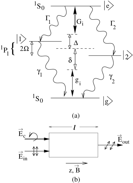
FIG. 1.: (a) The four-level model scheme (say of ${}^{40}Ca$) having $m$-degenerate sub-levels as its intermediate states. The symbols in left hand side denote the energy levels of ${}^{40}Ca$ atom. $2\Gamma_{i}$ and $2\gamma_{i}$ are the spontaneous decays, $2g_{i}$ ($2G_{i}$) is Rabi frequency of the probe (control) field due to coupling of the intermediate state $|i\rangle$ with $|g\rangle$ ($|e\rangle$). The detuning of probe (control) field from the center of $|1\rangle$ and $|2\rangle$ are represented by $\delta$ ($\Delta$). $2\Omega$ is the Zeeman split between the intermediate states. (b) A block diagram that shows the configuration under consideration. $\vec{B}$ defines the quantization axis $z$. The input probe $\vec{E}_{in}$ is $x$-polarized and the control field is left circularly polarized. Both the fields propagate along $z$. After passing through the cell, output is observed through a $y$-polarized analyzer.

FIG. 2.: Plots to show the control field induced birefringence in absence of magnetic field ($\Omega=0$). Control field is left circularly polarized and is in resonance with $|i\rangle\rightarrow|e\rangle$ transition ($\Delta=0$). In the above figure, first row refers to real and imaginary part $s^{-}$ (Eq.(29)) which is independent of the $\sigma_{-}$ control field. The frames ($a_{j}$), ($b_{j}$) and ($c_{j}$) represent Re $s^{+}$, Im $s^{+}$ and $T_{y}$ respectively. Three rows for $j=1,~{}2,~{}3$ correspond to control field strengths $G_{1}=20,~{}50,~{}100$ respectively. The x-axis represents the detuning of probe laser with respect to the position of the $j=1$ level with zero magnetic field.

FIG. 3.: Enhancement of MOR by use of a $\sigma_{-}$ control laser with the intermediate levels being split by a magnetic field with Zeeman splitting $2\Omega=10$. The graphs $(a_{j})$ and $(b_{j})$ represent the control field induced changes in Re $s^{+}$ and Im $s^{+}$ respectively and $(c_{j})$ represents the corresponding $T_{y}$, and $j=1,~{}2,~{}3$ refer to the case of resonant control field (i.e. $\Delta=\Omega$) with strengths $G_{1}=0,~{}20,~{}50$ respectively. Clearly large fields result in significant enhancement and in addition new regions appear with large MOR. Further enhancement is observed by use of a detuned laser as seen in frames ($c_{4}$) and ($c_{5}$) which are for $G_{1}=20$ and control laser detuning $\Delta=-20,~{}-30$ respectively.

FIG. 4.: Plots represent MOR enhancement with an elliptically polarized control (i.e. $G_{2}\neq 0$) and $\Delta=\Omega=5$. Here we have considered the case of $G_{2}=10$. The frames $(a_{j})$, $(b_{j})$, $(c_{j})$, $(d_{j})$ and $(e_{j})$ represent Re $s^{-}$, Im $s^{-}$, Re $s^{+}$, Im $s^{+}$ and $T_{y}$ respectively, and $j=1,~{}2,~{}3$ correspond to $G_{1}=0,~{}20,~{}50$ respectively. The off-resonant control field can also be advantageous (results not shown) as in Fig.3.

REFERENCES

• [1] J-P Connerade, J. Phys. B 16, 399 (1983); J-P Connerade, T. A. Stavrakas, and M. A. Baig, Synchrotron Radiation Sources and their Applications, ed. G. N. Greaves and I. H. Munro (Edinburgh: SUSSP Publications, Edinburgh University, 1989), p. 310; X. H. He and J-P Connerade, J. Phys. B 26, L255 (1993).
• [2] X. Chen, V. L. Telegdi, and A. Weis, Opt. Commun. 74, 301 (1990); E. Pfleghaar, J. Wurster, S. I. Kanorsky, and A. Weis, ibid 99, 303 (1993); A. J. Wary, D. J. Heading, and J-P Connerade, J. Phys. B 27, 2229 (1994).
• [3] D. S. Kliger, J. W. Lewis, and C. E. Randall, β€œPolarized light in optics and spectroscopy” (Academics Press, 1990).
• [4] For a recent review of MOR with laser sources see: W. Gawlik, in β€œModern Non-linear Optics”, ed. M. Evans, and S. Kielich, Advances in Chemical Physics Series vol. LXXXV, Part 3 (Wiley, New York, 1994).
• [5] G. S. Agarwal, P. Anantha Lakshmi, J-P Connerade, and S. West, J. Phys. B 30, 5971 (1997); P. Jungner, T. Fellman, B. Stahlberg, and M. Lindberg, Opt. Commun. 73, 38 (1989); K. H. Drake and W. Lange, ibid, 66, 315 (1988).
• [6] V. A. Sautenkov, M. D. Lukin, C. J. Bednar, G. R. Welch, M. Fleischhauer, V. L. Velichansky, and M. O. Scully, β€œEnhancement of Magneto-Optic Effect via Large Atomic Coherence”, quant-ph/9904032.
• [7] P. Avan and C. Cohen-Tannoudji, J. Physique Lett. 36, L85 (1975); S. Giraud-Cotton, V. P. Kaftandjian, and L. Klein, Phys. Rev A 32, 2211 (1985); F. Schuller, M. J. D. MacPherson, and D. N. Stacey, Opt. Commun. 71, 61 (1989).
• [8] S. P. Tewari and G. S. Agarwal, Phys. Rev. Lett. 56, 1811 (1986); G. S. Agarwal and S. P. Tewari, Phys. Rev. Lett. 70, 1417 (1993).
• [9] S. E. Harris, J. E. Field, and A. Imamoglu, Phys. Rev. Lett. 64, 1107 (1990); S. E. Harris, J. E. Field, and A. Kassapi, Phys. Rev. A 46, R29 (1992); S. E. Harris, Opt. Lett. 19, 2018 (1994); M. Jain, H. Xia, G. Y. Yin, A. J. Merriam, and S. E. Harris, Phys. Rev. Lett. 77, 4326 (1996).
• [10] M. O. Scully, Phys. Rev. Lett. 67, 1855 (1991); M. Fleischhauer, C. H. Keitel, M. O. Scully, Su Chang, B. T. Ulrich, and S. Y. Zhu, Phys. Rev A 46, 1468 (1992); M. O. Scully and M. Fleischhauer, Phys. Rev. Lett. 69, 1360 (1992); M. Fleischhauer and M. O. Scully, Phys. Rev. A 49, 1973 (1994); A. S. Zibrov, M. D. Lukin, L. Hollberg, D. E. Nikonov, M. O. Scully, H. G. Robinson and V. L. Velichansky, Phys. Rev. Lett. 76, 3935 (1996).
• [11] M. Xiao, Y. Li, S. Jin, and J. Gea-Banacloche, Phys. Rev. Lett. 74, 666 (1995).
• [12] S. Wielandy and A. L. Gaeta, Phys. Rev. Lett. 81, 3359 (1998); for yet another recent experiment similar to Gaeta’s experiment see: F. S. Pavone, G. Bianchini, F. S. Cataliotti, T. W. HΓ€nsch, M. Inguscio, Opt. Lett. 22, 736 (1997).
• [13] For some early studies of field induced birefringence see: P. F. Liao and G. C. Bjorklund, Phys. Rev. Lett. 36, 584 (1976); Y. I. Heller, V. F. Lukinykh, A. K. Popov, and V. V. Slabko, Phys. Lett. 82A, 4 (1981); A. E. Kaplan, Opt. Lett. 8, 560 (1983).
• [14] B. Stahlberg, P. Jungner, T. Fellman, K.-A. Suominen, and S. Stenholm, Opt. Commun. 77, 147 (1990); K.-A. Suominen, S. Stenholm, B. Stahlberg, J. Opt. Soc. America B 8, 1899 (1991). Here experimental and theoretical work on laser induced rotation is Ne is reported. The arrangement of fields is different - for example the $\sigma_{+}$ polarized probe does not interact with the system.