Star Formation in Galaxies with Large Lower Surface Brightness Disks

Abstract

We present B, R, and H$\alpha$  imaging data of 19 large disk galaxies whose properties are intermediate between classical low surface brightness galaxies and ordinary high surface brightness galaxies. We use data taken from the Lowell 1.8m Perkins telescope to determine the galaxies’ overall morphology, color, and star formation properties. Morphologically, the galaxies range from Sb through Irr and include galaxies with and without nuclear bars. The colors of the galaxies vary from B$-$R = 0.3 – 1.9, and most show at least a slight bluing of the colors with increasing radius. The H$\alpha$ images of these galaxies show an average star formation rate lower than is found for similar samples with higher surface brightness disks. Additionally, the galaxies studied have both higher gas mass-to-luminosity and diffuse H$\alpha$ emission than is found in higher surface brightness samples.

1 Introduction

Large low surface brightness galaxies are galaxies with disk central surface brightnesses statistically far from the Freeman (1970) value of $\mu_{B}(0)$ = 21.65 $\pm$ 0.3 mag arcsec^-2, and whose properties are significantly removed from the dwarf galaxy category (e.g. $M_{B}<-18$, $M_{\rm HI}>10^{9}$M_⊙). Studies of large LSB galaxies have discovered a number of intriguing facts: large LSB galaxies, in contrast to dwarf LSB galaxies, can exhibit molecular gas (Das, et al., 2006; O’Neil & Schinnerer, 2004; O’Neil, Schinnerer, & Hofner, 2003; O’Neil, Hofner, & Schinnerer, 2000); the gas mass-to-luminosity ratios of large LSB galaxies are typically higher than for similar high surface brightness counterparts by a factor of 2 or more (O’Neil, et al., 2004); and, like dwarf LSB galaxies, large LSB systems are typically dark-matter dominated (Pickering, et al., 1997; McGaugh, Rubin, & de Blok, 2001). These properties, added to their typically low metallicities (de Naray, McGaugh, & de Blok, 2004; Gerritsen & de Blok, 1999), lead to the inference that even large LSB galaxies are under-evolved compared to their high surface brightness (HSB) counterparts. Once their typically low gas surface densities (M${}_{HI}\leq 10^{21}\;\rm cm^{-2}$) (Pickering, et al., 1997) and low baryonic-to-dark matter ratios (Gurovich, et al., 2004; McGaugh, et al., 2000) are taken into account, the question becomes less why LSB galaxies are under-evolved than how they can form stars at all (O’Neil, Bothun, & Schombert, 2000, and references therein). Yet large LSB galaxies have the same total luminosity within them as ordinary Hubble sequence spirals (O’Neil, et al., 2004; Impey & Bothun, 1997; Pickering, et al., 1997; Sprayberry, et al., 1995). On average then, star formation cannot be too inefficient in these large LSB galaxies in spite of their unevolved characteristics, else their integrated light would be significantly less then in their HSB counterparts.

In an effort to better understand this enigmatic group of galaxies and their evolutionary status, we recently conducted a 21-cm survey to discover a larger nearby sample of such objects (O’Neil, van Driel, & Schneider, 2006; O’Neil, et al., 2004). We succeeded in identifying about 25 candidates within the redshift range $0.04<z<0.08$, whose combined HI and optical properties suggest them to be large LSB galaxies. We obtained B, R, and H$\alpha$ imaging of 19 of these galaxies at Lowell Observatory to confirm whether these candidates are indeed LSB galaxies, and to obtain a dataset of their fundamental parameters. These observations are presented here, and interestingly, none of the galaxies ultimately turned out to be LSB galaxies by the strict conventional definition; we discuss this result below in § 4. However, these galaxies still represent a sample whose surface brightnesses are below average, and whose properties are intermediate between those of the bona fide massive LSB galaxies, and ordinary HSB galaxies. In this work, we quantify and parameterize the fundamental properties of this sample of large, “lower surface brightness” galaxies.

2 Galaxy Sample

There are three ways that disk galaxy surface brightness can be measured or quantified – using a surface brightness profile and fitting an exponential disk to derive the central surface brightness; measuring an average surface brightness within a given isophotal diameter; and measuring the surface brightness of the isophote at the 1/2 light radius point (the effective surface brightness). The latter two definitions suffer from the fact that the bulge light is included in the surface brightness estimates, resulting in their prediction of the disk surface brightness to be less accurate. As a result, the typical operational definition of an LSB galaxy uses the first definition, and defines an LSB galaxy as one whose whose observed disk central surface brightness is $\mu_{B}(0)\geq$23.0 mag arcsec^-2. For reference, the Freeman value of $\mu_{B}(0)$=21.65 +/- 0.30 mag arcsec^-2 defines the distribution of central surface brightness, in the blue band, for Hubble sequence spirals.

Regardless of the definition, without pre-existing high quality optical imaging of galaxies, it is difficult to unambiguously identify a sample of disk galaxies that will turn out to be LSB. With only catalog data available, one is driven to use the average surface brightness and identify potential LSB galaxies as those whose average surface brightness is below some threshold level.

All of the galaxies in this sample were identified as LSB by Bothun, et al. (1985) using the magnitude and diameter values found in the Uppsala General Catalog (Nilson, 1973), and employing the general equation $\langle\mu_{B}\rangle=m_{pg}+5log(D)+8.63$. Here, $m_{pg}$ is the photographic magnitude of the galaxies, D is the diameter in arcminutes, and the constant, 8.63, is derived from the conversion from arcminutes to arcseconds (8.89) and the conversion from m_pg to m_B (-0.26, as used by Bothun, et al.) Bothun, et al. (1985) then made a cut-off to the galaxies in their sample, requiring $\langle\mu_{B}\rangle>$24.0 mag arcsec^-2 to look for galaxies with lower surface brightness disks, with the majority of the galaxies chosen having $\langle\mu_{B}\rangle>$25.0 mag arcsec^-2 . (The inclusion of a number of galaxies with $\langle\mu_{B}\rangle$=24-25 mag arcsec^-2 was due to the 0.5mag errors given in the UGC.)

The Bothun, et al. (1985) sample was further pared down by our desire to image large LSB galaxies. That is, we wished to avoid the dwarf galaxy category entirely. To do this, we required the galaxies to have M${}_{HI}>10^{9}$ M_⊙, W${}_{20}>$ 200 km s^-1, and/or M${}_{B}<-19$. These criteria are sufficiently removed from the dwarf galaxy category to guarantee no overlap between our sample and that category exists.

3 Observations & Data Reduction

Galaxies’ integrated broad-band colors represent a convolution of the mean age of the stellar population, metallicity, and recent star formation rate; while measurements of H$\alpha$ luminosity provide a direct measure of the current star formation rate (SFR). With these combined observations, is is possible to parameterize the current SFR relative to the overall star formation history. As a result, these observations are widely used in many surveys that target fundamental galaxy parameters, for example, SINGG (Meurer, et al., 2006) and 11HUGS (Kennicutt, et al., 2004), and others (e.g. Gavazzi, et al., 2006; Koopman & Kenney, 2006; Helmboldt, et al., 2005).

19 galaxies were observed on 7-10 June, 2002 and 5-8 October, 2003 using the Lowell 1.8m Perkins telescope. The filter set used included Johnson B and R as well as three H$\alpha$ filters from a private set (R. Walterbos) with center frequency/bandwidths of 6650/75, 6720/35, 6760/75 Å. A 1065x1024 pixel Loral SN1259 CCD camera was used, giving a 3.3^′ field of view and resolution of 0.196^′′/pixel. Seeing in June, 2002, ranged from 1.8^′′ - 2.4^′′ and from 1.4^′′ - 2.2^′′ for the October, 2003, observations. At least 3 frames, each shifted slightly in position, were obtained for each object through each filter and were median filtered to reduce the effect from cosmic rays, bad pixels, etc. All initial data reduction (bias and flat field removal, image alignment, etc) was done within IRAF. The R band images were scaled and used as the continuum images for data reduction purposes.

Corrections to the measured fluxes were made in the following way. Atmospheric extinction was obtained using the observational airmass and the atmospheric extinction coefficients for Kitt Peak which are distributed with IRAF. Galactic extinction was corrected using the values for E(B$-$V) obtained from NED, the reddening law of Seaton (1979) as parameterized by Howarth (1983) ($A(\lambda)=X(\lambda)E(B-V)$) and assuming the case B recombination of Osterbrock (1989) with R_V=3.1 (O’Donnell, 1994) (X(6563Å)=2.468). Contamination from $\left[{NII}\right]$ emission in the H$\alpha$ images was corrected using the relationship derived by Jansen, et al. (2000) and re-confirmed by Helmboldt, et al. (2004):

$$log{{\left[NII\right]}\over{H\alpha}}=\left[-0.13\pm 0.035\right]M_{R}+\left[-3.2\pm 0.90\right],$$

where $M_{R}$ is the absolute magnitude in the R band. H$\alpha$ extinction was determined using the equation found in Helmboldt, et al. (2004):

$$log\left(H\alpha\right)_{int}=\left[-0.12\pm 0.048\right]M_{R}+\left[-2.5\pm 0.96\right]$$

which was found through a linear least squares fitting to the $A(H\alpha)_{int}$ determined using all galaxies in his sample with a measured H$\beta$ flux. For this calculation, Helmboldt, et al. (2004) used the H$\alpha$ to H$\beta$ ratio measured by Jansen, et al. (2000), an assumed intrinsic ratio of ${{H\alpha}\over{H\beta}}$=2.85 (Case B recombination and T=10⁴ K (Osterbrock, 1989)), the extinction curve of O’Donnell (1994), and R_V=3.1 No correction for internal extinction due to inclination was made for the B and R bands. It should be noted, though, that in a number of plots inclination corrections were made to the B and R colors and central surface brightnesses, as noted in the Figure captions. The corrections used in these cases are:

$$\mu(0)^{\lambda}_{corr}=\mu(0)^{\lambda}-2.5C^{\lambda}log(b/a)$$ (1)

and

$$m^{\lambda}_{corr}=m^{\lambda}-A^{\lambda}$$ (2)

$$A^{\lambda}=-2.5log\left[f\left(1+e^{-\tau^{\lambda}sec(i)}\right)\>+\;\left(1-2f\right)\left({{1-e^{-\tau^{\lambda}sec(i)}}\over{\tau^{\lambda}sec(i)}}\right)\right]$$ (3)

Here, C^R,B=1 (Verheijen, 1997); $\left(b/a\right)$ is the ratio of the minor to major axis; f = 0.1 and $\tau_{R,B}$=0.40, 0.81 (Tully, et al., 1998; Verheijen, 1997). Finally, a correction was applied to account for the effect of stellar absorption in the Balmer line of

$$F_{cor}=F_{obs}\left({1+{{W_{a}}\over{W_{e}}}}\right),$$ (4)

where $F_{cor}$ is the corrected and $F_{obs}$ is the observed H$\alpha$ flux, W_e is the measured equivalent width and W_a is the equivalent width of the Balmer absorption lines. As we do not have measurements for W_a, we estimated W_a to be 3$\pm$1 Å, based off the values found in Oey & Kennicutt (1993); Roennback & Bergvall (1995); McCall, Rybski, & Shields (1985). Note that this effect is potentially stronger in the diffuse gas than in the H II regions due to the older stellar population likely lying in the diffuse gas. As a result we may still be underestimating the total H$\alpha$ flux in the diffuse gas within the galaxies. However, as the diffuse gas fractions for these galaxies are extremely high (see Section 6, below), it is unlikely that this effect is high.

Global parameters and radial profiles for the galaxies were determined primarily using the routines available in IRAF (notably ellipse) and the results are given in Tables 1 and 2. Galaxy images, surface brightness profiles, and color profiles are given in Figures 1 – 3. In all cases the inclination and position angle for the galaxies were determined from the best fit values from the B & R frames. These best fit values were then used for the ellipse fitting in all four images (B, R, H$\alpha$  and continuum with H$\alpha$ subtracted), a practice which insures the color profiles are obtained accurately and are not affected by, e.g. misaligned ellipses. The same apertures were also used for all four images, with the apertures found through allowing ellipse to range from 1 pixel (0.196^′′) until the mean value in the ellipse reaches the sky value, increasing geometrically by a factor of 1.2. Sky values were found through determining the mean value in more than 100 5$\times$5 sq. pixel boxes in each frame. The error found for the sky was incorporated into all magnitude and surface brightness errors, which also include errors from the determination of the zeropoint and the errors from the N II contribution to the H$\alpha$ (in the case of the H$\alpha$ magnitudes).

The B and R surface brightness profiles of all galaxies were fit using two methods. First, the inner regions of the galaxies’ surface brightness profiles was fit using the de Vaucouleurs r^1/4 profile

$$\Sigma(r)=\Sigma_{eff}exp^{-7.669\left[{(r/r_{eff})^{1/4}-1}\right]}\rightarrow\mu(r)=\mu_{eff}+8.327\left[{\left({{r}\over{r_{eff}}}\right)}^{1/4}-1\right],$$ (5)

and the outer regions were fit by the exponential disk profiles

$$\Sigma(r)=\Sigma_{0}exp^{\left({{r}\over{\alpha}}\right)}\rightarrow\mu(r)=\mu_{0}+1.086\left({{r}\over{\alpha}}\right).$$ (6)

Additionally, we attempted to fit a disk profile (6) to both the inner and outer regions of the galaxies’, to determine if a two-disk fit would better match the data (Broeils & Courteau, 1997; de Jong, 1996). Roughly one-fourth of the galaxies (5/19) were best fit (in the $\chi^{2}$-sense) by the standard bulge+disk model. Another 47% of the galaxies were best fit by the two-disk model. Of the remaining galaxies, 21% (4 galaxies) were best fit by a single disk, and one galaxy (UGC 11840) could not be fit by any profile. The results from the fits are shown in Table 3 and Figure 2, and an asterisk (*) is placed next to the best fit model. Note that in a few cases (e.g. UGC 00189) only one model is listed in the Table. This is due to the fact that in these cases the fitting using the other model proved to be completely unrealistic. Finally, it should be noted that in all cases the same best-fit model was used for both the B and R data.

The color profiles were similarly fit (using an an inverse error weighting) with a line to both the inner and outer galaxy regions (Figure 3). Here, though, the “boundary radius” was simply taken from the surface brightness profile fits, with the “boundary radius” being defined as the radius where the inner and outer surface brightness fits crossed. If only one (or no) fit was made to the surface brightness profile, then only one color profile was fit. In a number of cases the difference in slope between the inner and outer galaxy regions was less than the least-squares error for the fit. In these cases again only one line was fit for the color profiles.

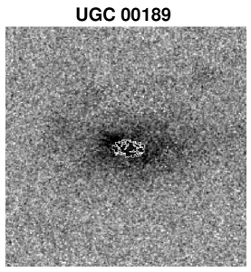
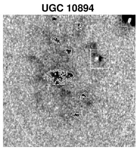
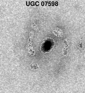
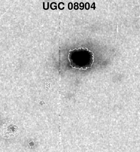
Figure 4: Example images showing the H II regions found by HIIphot for the galaxies UGC 00189, UGC 10894, UGC 07598, and UGC 08904. The H II regions are outlines in white. In the case of UGC 10894 two regions which were masked due to the presence of stars can also be seen, outlined by the square white boxes.

The HIIphot program (Thilker, Braun, & Walterbos, 2000) was used both to determine the shape and number of H II regions for each galaxy and also to determine the H$\alpha$ flux for each of these regions. The fluxes from the H$\alpha$, H$\alpha$-subtracted continuum, B, and R images were measured in identical corresponding apertures, which are the H II region boundaries defined by HIIphot. While HIIphot applies an interpolation algorithm across these apertures to estimate the diffuse background in the H$\alpha$ frames, we determined the background in other bands from the median flux in an annulus around each H II region aperture. Results from the analysis of the H II regions are given in Table 4, and sample H II regions are shown in Figure 4. Errors for the H$\alpha$, SFR, and EW measurements are derived from the error values reported with HIIphot. Errors for the B and R magnitudes, and colors, are derived from the total sky and zeropoint errors, as well as the error in positioning of the HII regions. The diffuse fraction errors are derived both from the total H$\alpha$ flux errors and also include errors in determining the total flux within the HII regions and for the entire galaxy. Finally, it should be mentioned that the equivalent width (EW) was calculated simply as the ratio of the H$\alpha$ flux to H$\alpha$-subtracted continuum flux for a given region (or the whole galaxy).

The large distances to the observed galaxies (40 - 100 Mpc) results in many of the H II region being blended together. As a result, any luminosity function derived for these objects would be necessarily skewed towards larger HII regions (see Oey, et al., 2006). This can be seen in the analysis done by Thilker, Braun, & Walterbos (2000) wherein the dependence of the luminosity function found for M51 was examined. There one can clearly see the increase in the number of high luminosity regions and subsequent reduction in the number of low luminosity regions as the galaxy is ’moved’ to increasing distances. Examining their results also shows that while the distribution of H II region luminosities changes with distance, the total luminosity of the H II regions, as found by HIIphot, does not change significantly as the galaxy moves from 10 Mpc to 45 Mpc. As a result, while determining luminosity functions for the galaxies in this paper is not feasible due to the distances involved, derivations such as the diffuse fraction are unaffected by distance. This fact is also supported by the SINGG survey results (Oey, et al., 2006).

4 Surface Brightness

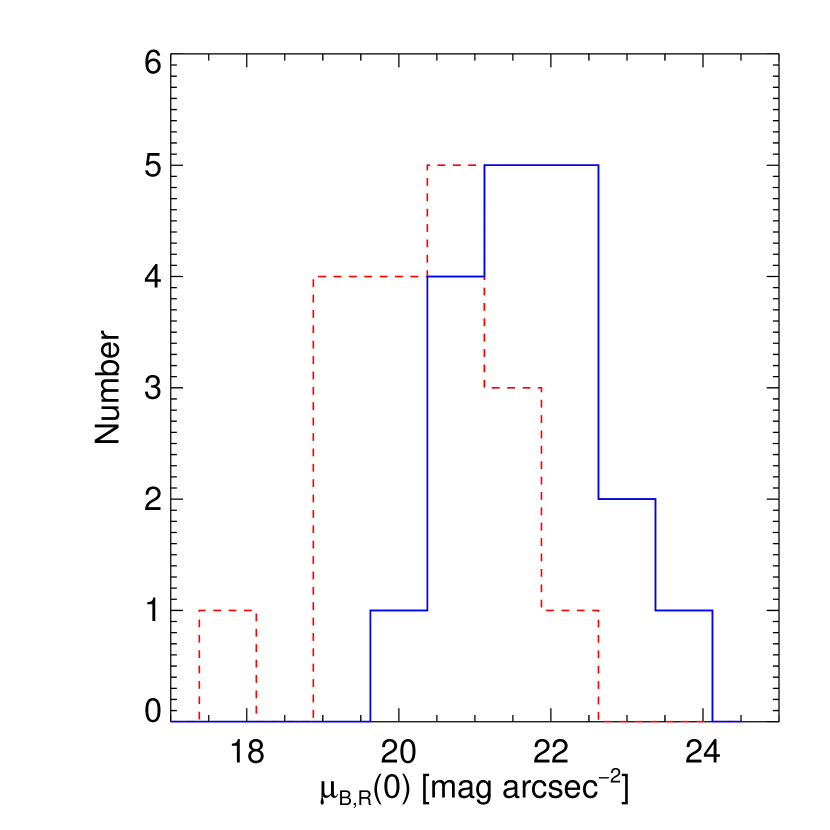
Figure 5: (Left) Histogram showing the distribution of central surface brightnesses for the observed galaxies. The (red) dashed line shows the R-band data and the (blue) solid line shows the B-band data. (Right) Plot of the observed central surface brightness against scale length of the outer disk. Here, the R-band data is demarcated by (red) open circles while the B-band data uses (blue) filled circles.

The distribution of central surface brightnesses found for the galaxies observed is shown in Figure 5. As is plain from that Figure, the mean measured central surface brightness for this sample, falls short of the definitions discussed in Section 2. Indeed only 4 galaxies in our sample meet the operational definition of LSB galaxies as having $\mu_{B}(0)\geq$ 23 mag arcsec^-2. If we return to the Freeman value, however, we see that the operational definition of LSB galaxies is 4.5$\sigma$ from the value for Hubble sequence spirals, making it statistically extreme. For the sample defined here, half have central surface brightnesses at least two sigma above the Freeman value, a definition only 2.5% of the Freeman sample meets. As a result, while the sample does not meet the operation criteria for LSB galaxies, we clearly do have a sample with lower central surface brightnesses that would be found in the average Hubble sequence galaxies.

It should be pointed out here that the main scientific focus of Bothun, et al. (1985) was not oriented toward producing a representative sample of LSB galaxies as detected on photographic surveys (that focus did not occur until Schombert & Bothun, 1988), but rather toward identifying cataloged galaxies for 21-cm based redshift determinations. The galaxies were chosen to have surface brightnesses that were too low for reliable optical spectroscopy (assuming emission lines were not present). This was done as a test of the potentially large problem of bias in on going optical redshift surveys in the time (see Bothun, et al., 1986). In fact, the operational criteria for selecting the galaxies that were observed at Arecibo 20 years ago, lay in the knowledge that these cataloged galaxies were never going to be even attempted in the optical redshift surveys of the time and this raised the very real possibility of biased redshift distributions and an erroneous mapping of large scale structure.

In the original redshift measurements of Bothun, et al. (1985) a significant number of candidate LSB galaxies were not detected at 21-cm within the observational redshift window (approximately 0-12,000 km/s). Many of those non-detections would later turn out to be intrinsically large galaxies located at redshifts beyond 12,000 km/s (see O’Neil, et al., 2004). As we are interested here in the H$\alpha$ properties of galaxies with large, relatively LSB disks, these initial non-detections comprise the bulk of our sample.

Surface photometry of this sample not only provides detailed information regarding the galaxies’ surface brightness and color distributions, but it also probes the efficacy of the Bothun, et al. (1985) average surface brightness criteria for selecting LSB disks. Here, we used the magnitudes and diameters obtained in this study (Table 1) with two different equations for determining a galaxy’s average surface brightness within the D₂₅ radius. The first equation used is that of Bothun, et al. (1985)

$$\langle\mu_{25}\rangle=m_{25}+5log(D_{25})+3.63$$ (7)

and the second is a modified version of the above equation from Bottinelli, et al. (1995) which takes the galaxies’ inclination into account:

$$\langle\mu_{25}\rangle=m_{25}+5log(D_{25})+3.63-2.5log\left[kR^{-2C}+\left(1-k\right)R^{(0.4C/K)-1}\right].$$ (8)

In both equations, m₂₅ and D₂₅ are the magnitude and diameter (in units of 0.1^′) at the $\mu$=25.0 mag arcsec^-2 isophote, R is the axis ratio (a/b), and C is defined as (logD/logR) and is fixed at 0.04 (Bottinelli, et al., 1995). Finally, k (the ratio of the bulge-to-disk luminosity) and K (a measure of how the apparent diameter changes with surface brightness at a given axis ratio) are dependent on the revised de Vaucouleurs morphological type (T) as follows (Simien & de Vaucouleurs, 1986; Fouqué & Paturel, 1985):
T=1 $\rightarrow$ k=0.41; T=2 $\rightarrow$ k=0.32; T=3 $\rightarrow$ k=0.24; T=4 $\rightarrow$ k=0.16; T=5 $\rightarrow$ k=0.09; T=6 $\rightarrow$ k=0.05; T=7 $\rightarrow$ k=0.02; T$\geq$8 $\rightarrow$ k=0.0;

$$K=0.12-0.007T\>\;if\>\;T<0;\>K=0.094\>\;if\>\;T\geq 0.$$

The values for k at T$\geq$8 are extrapolated from fitting the Simien & de Vaucouleurs (1986) values.

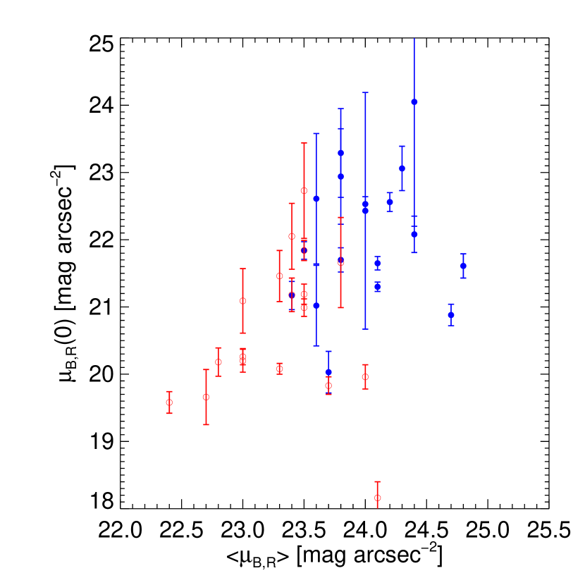
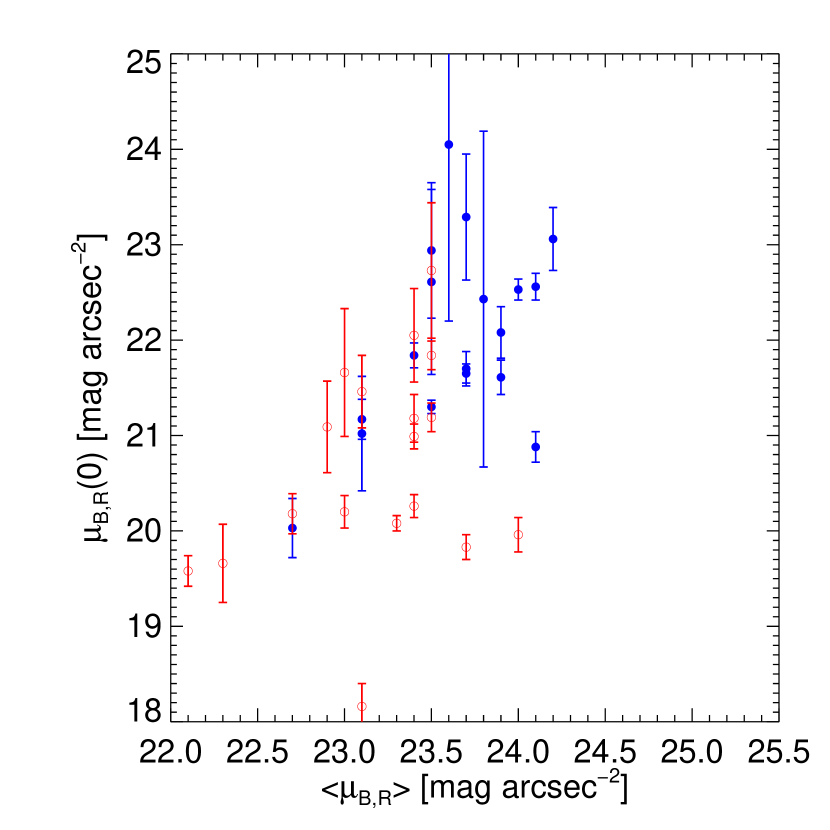
Figure 6: Plots comparing the measured central surface brightnesses with the average surface brightness for the galaxies, as defined by Equation 7 (left) and Equation 8 (right) and using the magnitude and diameter values found herein. The R-band data is demarcated by (red) open circles while the B-band data uses (blue) filled circles.

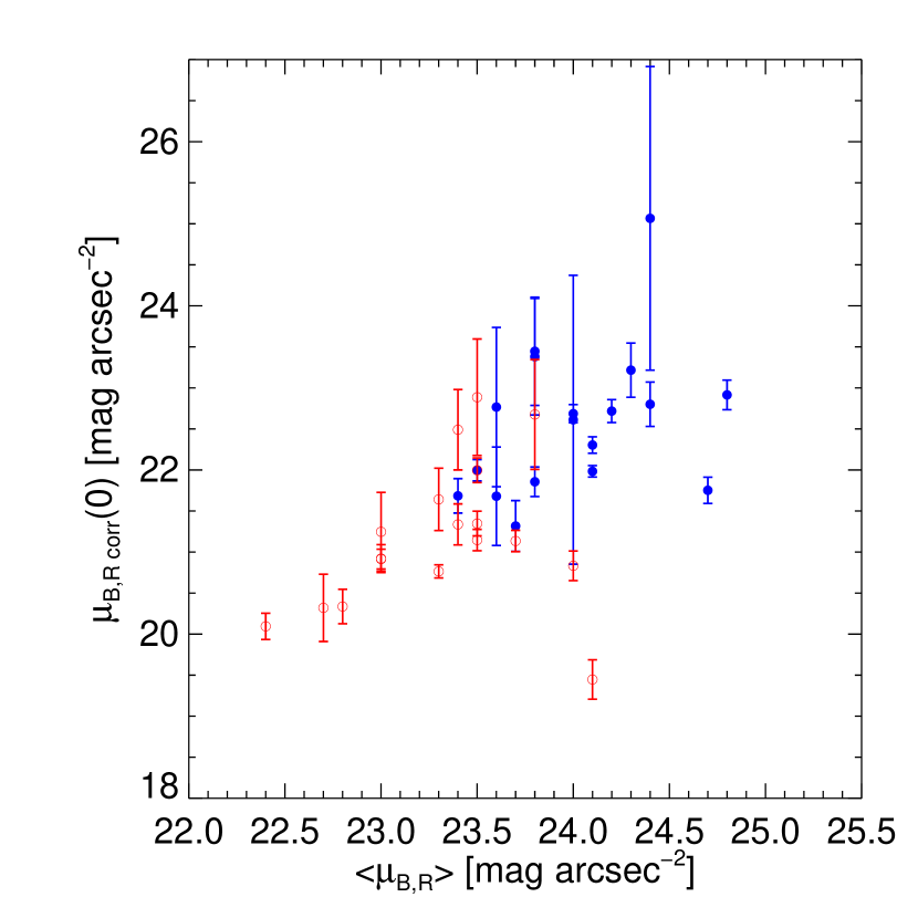
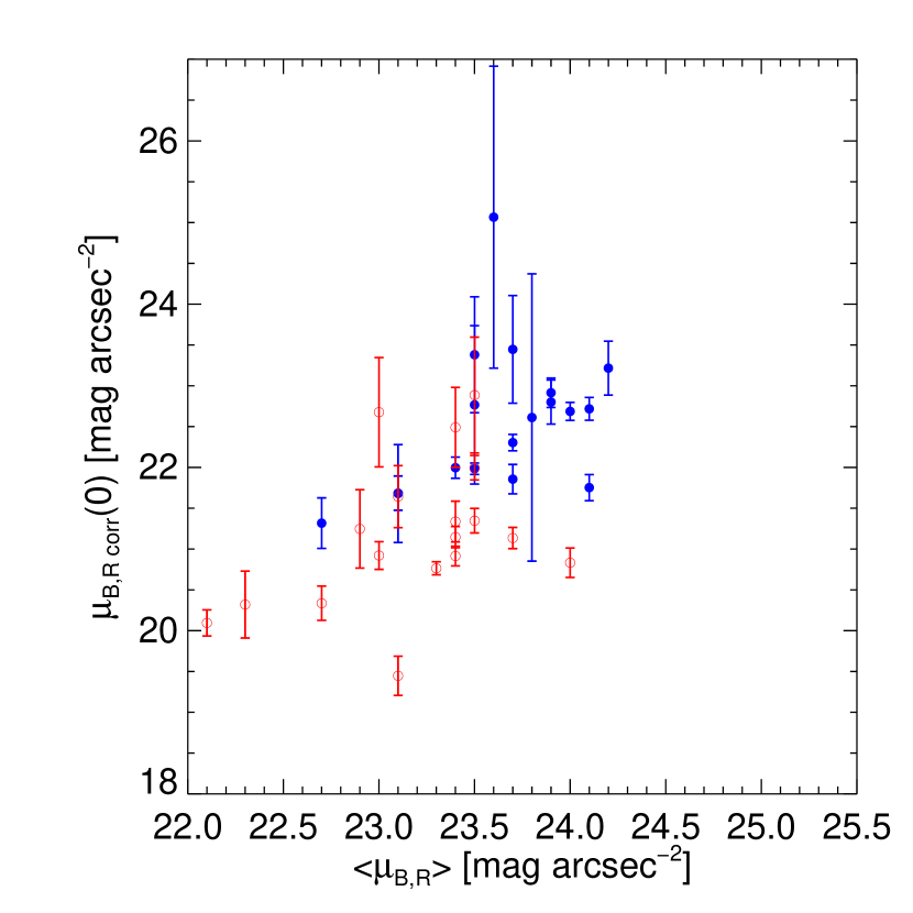
Figure 7: Plots comparing the measured central surface brightnesses, corrected for inclination, with the average surface brightness for the galaxies, as defined by Equation 7 (left) and Equation 8 (right) and using the magnitude and diameter values found herein. The R-band data is demarcated by (red) open circles while the B-band data uses (blue) filled circles.

The results of equations 7 and 8, plotted against the galaxies’ central surface brightness both uncorrected and corrected for inclination, are shown in Figures 6 and 7, respectively. The difference between the two plots is small, with neither equation doing an excellent job in predicting when a disk’s central surface brightness will be low. The two equations (Bothun, et al. (1985) and Bottinelli, et al. (1995)) have roughly the same fit (in the $\chi^{2}$ sense), which at first appears surprising. It is likely that uncertainties in the inclination measurements and morphological classification of the galaxies have increased the scatter in the Bottinelli, et al. (1995) equation, increasing the scatter in an otherwise more accurate equation. As a result, while the Bottinelli, et al. (1995) may indeed be the most accurate, the simpler equation is equally as good to use in most circumstances as it involves fewer assumptions.

The second fact that is readily apparent in looking at Figures 6 and 7 is that with the new measurements of magnitude and diameter, none of the galaxies in our sample meet the criterion laid out by Bothun, et al. (1985) for an LSB galaxy. That is that none of the galaxies in this sample have $\langle\mu_{25}\rangle>$25 mag arcsec^-2. As Bothun, et al. (1985) listed all of these objects as having $\langle\mu_{25}\rangle\;>$25 mag arcsec^-2 using the magnitudes and diameters provided by the original UGC measurements, this shows that the UGC measurements indeed predicted fainter magnitudes/larger values for D₂₅ than is found with more sophisticated measurement techniques. Additionally, it is good to note that the trends shown in Figures 6 and 7 indicate that any galaxy which met the $\langle\mu_{25}\rangle>$25 mag arcsec^-2 criteria would be highly likely to also have $\mu(0)>$23 mag arcsec^-2.

In these days of digital sky surveys it is difficult to appreciate the immense undertaking that defines the UGC catalog. Anyone who has looked at the Nilson selected galaxies on the Palomar Observatory Sky Survey (POSS) plates with a magnifying eyepiece really has to marvel that Nilson’s eye saw objects at least one arcminute in diameter. It is thus not surprising that, at the ragged end of that catalog, many of the listed UGC diameters are systematically high. Cornell, et al. (1987) made a detailed diameter comparison between diameters as obtained from high quality CCD surface photometry and the estimates made by Nilson (1973). They compared the diameter at the 25.0 mag arcsec^-2 isophote in CCD B images to the tabulated diameter in the UGC. The study, based on approximately 250 galaxies, identified two sources of systematic error (neither of which are surprising). First, galaxies with reported diameters less than 2^′ typically had D_25,B as measured by the CCD images that were 15-25% smaller. Second, Cornell, et al. (1987) found a systematic bias as a function of surface brightness in the sense that lower surface brightness galaxies had a higher number of overestimated diameters in the UGC than higher surface brightness galaxies. It should also be noted that the majority of the galaxies in this study lie at low Galactic latitude. This seems to be a perverse consequence that there is a large collection of galaxies between 7,000 – 10,000 ${\rm km\,s}^{-1}$ (where the diameter criterion in the UGC yields a relatively large physical size) located at relatively low galactic latitude. Nominal corrections for galactic extinction made by Bothun, et al. (1985) turned out to underestimate the extinction as shown by later published extinction maps. In some cases, the differences were as large as one magnitude. The combination of these facts with the very uncertain magnitudes of many of these galaxies (see Bothun & Cornell, 1990), it is not surprising that the measured average surface brightness could easily be 1-1.5 magnitudes higher than the average surface brightness that has been estimated from the UGC catalog parameters (roughly 40% of this comes from systematic magnitude errors and 60% from the diameter errors discovered by Cornell, et al. (1987)).

5 Morphology & Color

All of the galaxies observed have large sizes ($3\alpha_{B}$ = 10 – 54 kpc), bright central bulges, and well defined spiral structure (Figure 1). In most cases the galaxies can be described as late-type systems (Sbc and later). There are, though, a number of exceptions to this rule. Three of the galaxies, UGC 00023, UGC 07598, and UGC 11355 (Sb, Sc, and Sb galaxies, respectively) have clear nuclear bars. UGC 08311, classified as an Sbc galaxy, is clearly in the late stages of merging with another system. In this case the LSB classification of the galaxy is likely bogus, as the apparently LSB disk is likely just the remnant the merging process and will disappear as the galaxy compacts after the merging process. UGC 8904 is given a morphological type of S? with both NED and HYPERLEDA, yet the faint spiral arms surrounding it indicate its should be properly classified as an Sbc system. UGC 12021 is, like UGC 00023, listed as an Sb galaxy. Finally, UGC 11068 has a faint nuclear ring which is most readily visible in the B image.

The differences between the galaxies becomes more apparent when the H$\alpha$ images are examined. Hodge & Kennicutt (1983) classify the radial distribution of H II regions in spiral galaxies into three broad categories – galaxies with H II region surface densities which decrease with increasing radius, galaxies with oscillating H II region surface densities, and galaxies with ring-like H II density distributions. To these categories we would add a fourth, to include those galaxies with no detectable H II regions.

The first category of Hodge & Kennicutt (1983) is also the most common, as it includes all galaxies with generally decreasing radial densities of H$\alpha$. In the Hodge & Kennicutt (1983) sample this category is dominated by Sc – Sm galaxies but contains all Hubble types. In our sample, this category includes both galaxies with and without significant H$\alpha$ emission in the spiral arm regions. This group includes UGC 00023, UGC 00189, UGC 02588, UGC 02796, UGC 03119, UGC 03308, UGC 07598, and UGC 12021. Interestingly, of the galaxies listed above, 4/8 are Sb/Sbc galaxies and 3/8 are Sc-Sm galaxies. (The last galaxy, UGC 02588, is an irregular galaxy.)

The second category of Hodge & Kennicutt (1983), galaxies with oscillating densities, is dominated in their sample of Sb galaxies. Only a few of the galaxies in this sample fall into this category, 80% of which are also Sb/Sc galaxies. These are UGC 02299, UGC 08311, UGC 08904, UGC 11355, and UGC 11396. These galaxies all have a concentration of star formation seen in the nuclear regions and then clumps of star formation spread through the spiral arms, typically accompanied by diffuse H$\alpha$ also spread throughout the arms.

The third category of Hodge & Kennicutt (1983) is dominated by early-type galaxies, of which we have none in our sample. Nonetheless we have three galaxies which fall into this category – UGC 08644, UGC 10894, and UGC 11617. All three have H II regions spread throughout their disks, with no central concentration near the galaxies’ nuclei. In fact, the three brightest star forming regions within UGC 08644 all lie with the spiral arms, and are visible in all three filters. In contrast, both UGC 11617 and UGC 10894 have no bright H II regions, but instead have a large number of diffuse H II regions, with the brightest (as listed in Table 2) receiving that designation simply due to its size.

The fourth category of galaxies contains UGC 01362, UGC 11068, and UGC 11840, none of which have detectable H$\alpha$. In the case of UGC 01362 and UGC 11840 this is not too surprising as the galaxies are dominated by a bright nucleus, and their surrounding spiral arms are extremely faint in both R and B. As a result, any H$\alpha$ which may exist in the galaxies’ disks is too diffuse to be detected. UGC 11068, though, has both a well defined nucleus and a clear spiral structure extending out to a radius of $\sim$13 kpc (3$\alpha$). Yet no H$\alpha$ can be detected in this galaxy. This may mean that UGC 11068 is in a transition state for its star formation, with no ongoing star formation yet with enough recent activity that the spiral arms remain well defined.

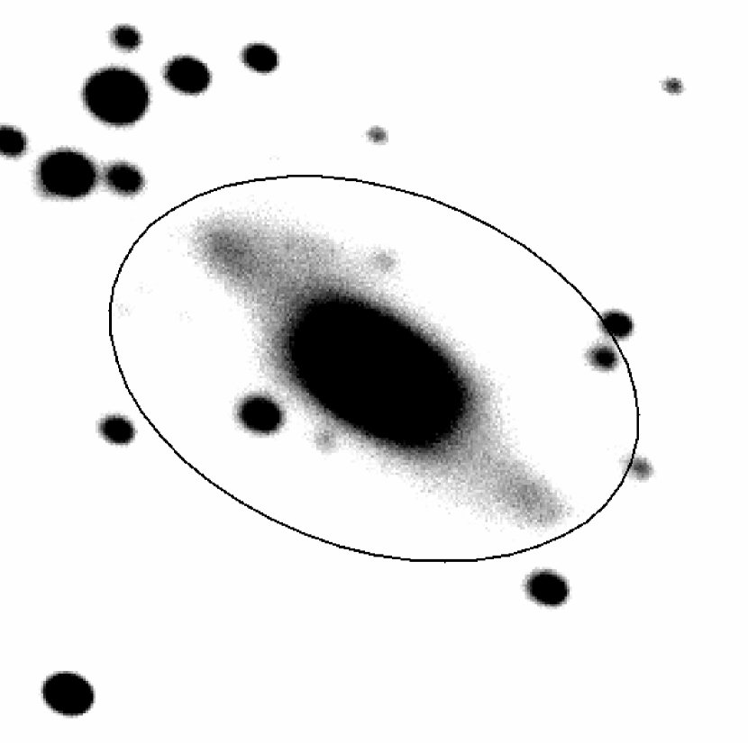
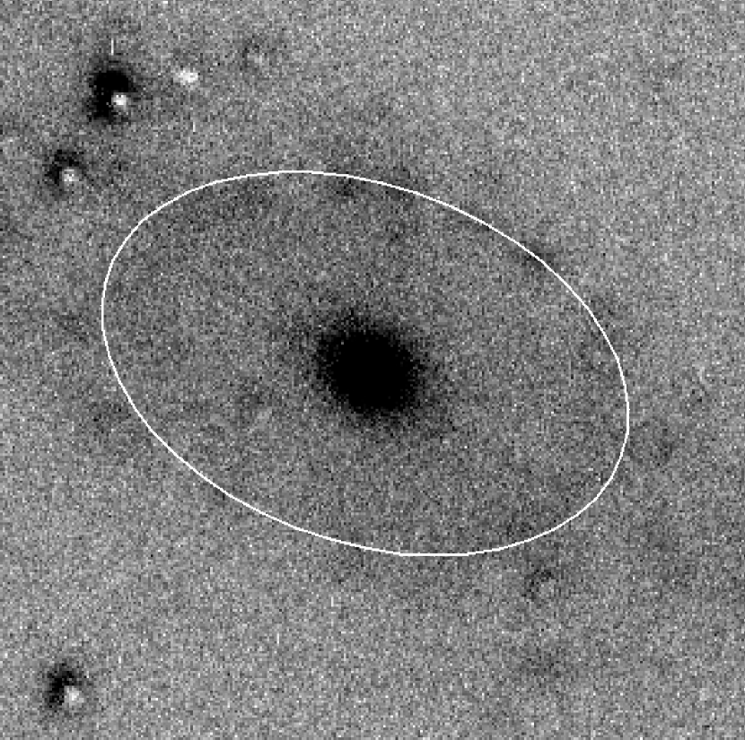
Figure 8: Images of UGC 11355 with the stretch altered to show the galaxy’s nuclear bar (left - R-band image) and star forming ring (right - H$\alpha$ image). In both images the ellipse shows the shape and size of the star forming ring. The images are 1.0^′ across.

Perhaps the most intriguing galaxy of our sample is UGC 11355. This galaxy was placed in Category 2, above, as it has a bright nucleus and clumpy disk in the H$\alpha$ image. The B and R band images of UGC 11355 show a galaxy with a simple Sbc morphology. The H$\alpha$ image, though, shows a distinct star forming ring. The ring is at a very different inclination from the rest of the galaxy (i=49^∘ for the ring and 73^∘ for the galaxy as a whole), and lies approximately 2.6 kpc in radius from the center of the galaxy, measured along the major axis. As the B and R images show no indication of a ring morphology this indicates unusually strong star formation in the ring. It is also useful to note the presence of a bar in UGC 11355 – shown more clearly in Figure 8. The fact that the inclination of the ring is significantly different from that of the rest of the galaxy suggests the ring a tidal effect due to an interaction, such as a small satellite galaxy being cannibalized by UGC 11355, or the influence of CGCG 143-026, 14.9^′ and 68 ${\rm km\,s}^{-1}$ away.

It is interesting to note that the H$\alpha$ morphology of the galaxies does not appear to correlate with the galaxies’ color profile (Figure 3). The galaxy with the steepest slope in the color profile is UGC 08644 which has only a few H II regions in its outer arms. The other galaxies with steep color profiles are UGC 00023 and UGC 8904, which have a bright knot of star formation in the nucleus and faint H$\alpha$ spread throughout their arms, and UGC 11840 and UGC 11068 both of which have no detectable H$\alpha$. The galaxies with the shallowest slopes similarly show no correlation between their color profiles and morphology. This suggests that the current star formation in these galaxies is largely independent of the past star-formation history, although this result should be confirmed with better, extinction-corrected, data.

6 Star Formation

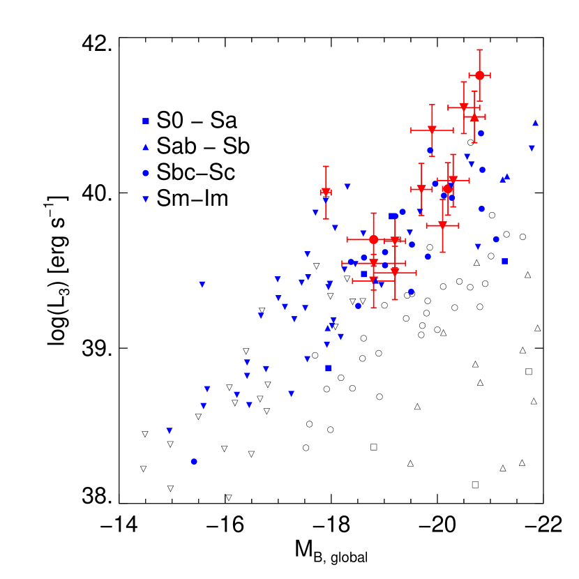
Figure 10: Total B magnitude plotted against the average luminosity of the brightest three H$\alpha$ regions. (If less than three regions were found, the average of all H II regions was used.) The filled (red) symbols are the data from our observations; the filled (blue) symbols are from Helmboldt, et al. (2005); and the open (black) symbols are from Kennicutt & Kent (1983).

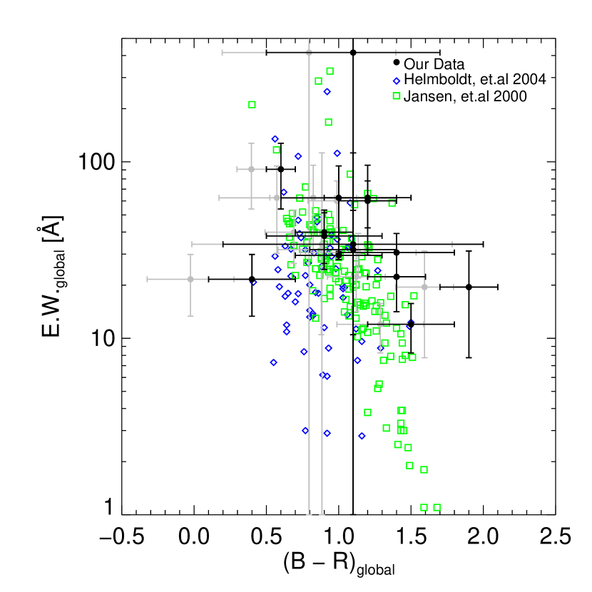
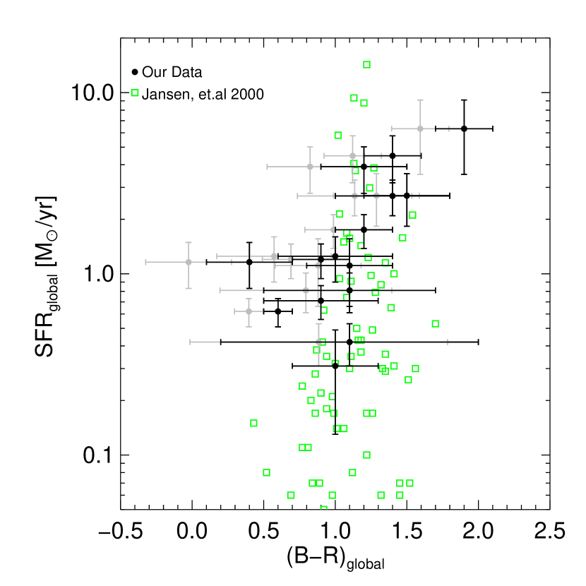
Figure 11: Global color versus equivalent width (left) and star formation rate (right). To insure any trends (or lack) remain the same, the data from this paper is shown both without inclination correction (black) and with (gray). Note that inclination corrections are described in Section 3. As the global SFR was not available for the Helmboldt, et al. (2005) data, it is not shown on the right.

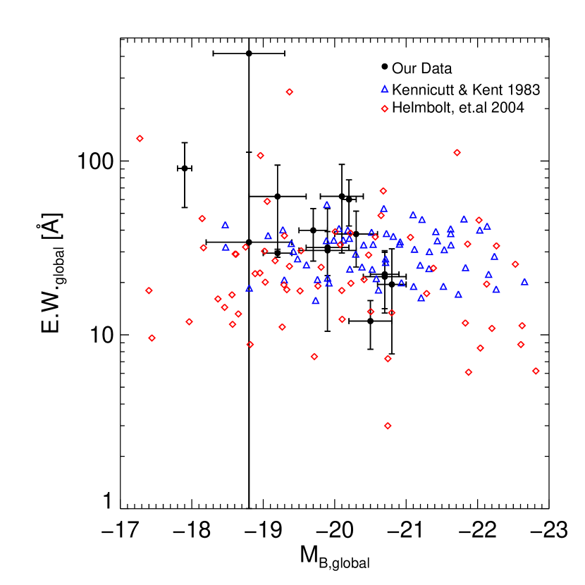
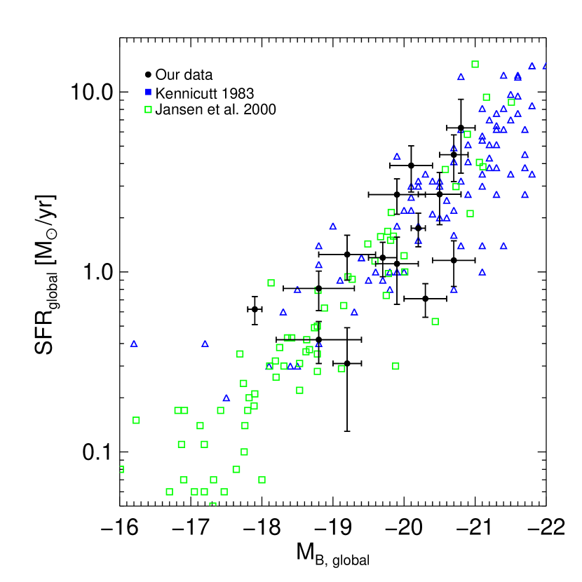
Figure 12: Total B magnitude plotted against the global equivalent width (left) and star formation rate (right). As the global SFR was not available for the Helmboldt, et al. (2005) data, it is not shown on the right.

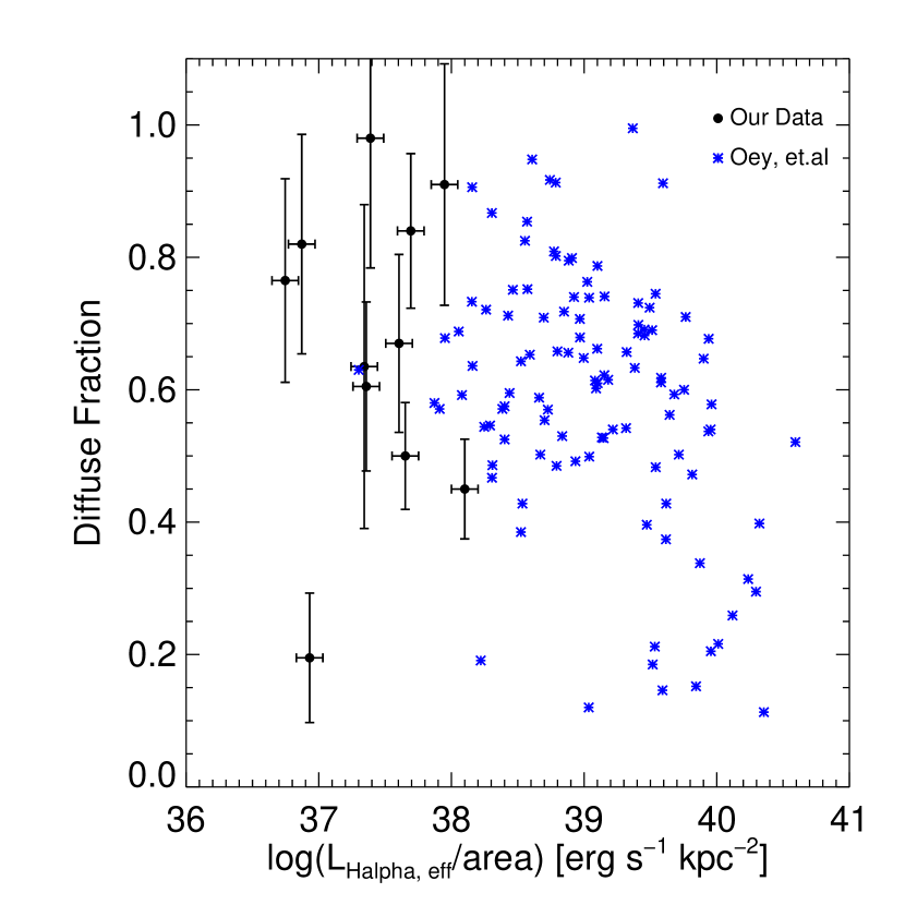
Figure 13: Luminosity surface brightness (Luminosity/area) plotted against the diffuse H$\alpha$ fraction for our sample and that of Oey, et al. (2006).

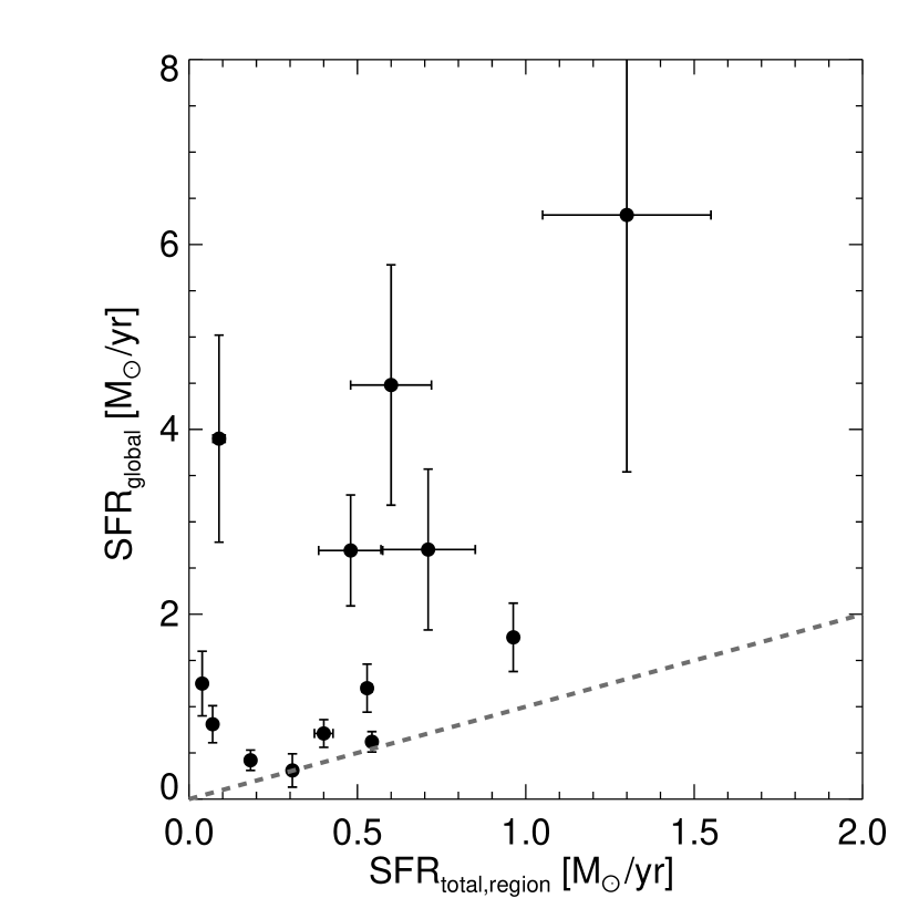
Figure 14: A comparison of regional and global star formation rate and equivalent width for the studied galaxies. On the left is a plot of the global SFR against the total SFR found for the individual H II regions, with a line demarcating the point where the global and regional SFR are equal. On the right is a plot of the global EW against the average EW for the individual H II regions.

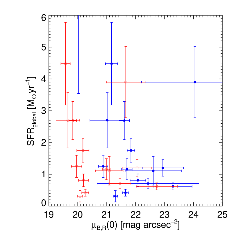
Figure 15: Central surface brightness versus global star formation rate for the observed galaxies. The (red) open circles are from the R band data, while the (blue) filled circles are for the B data.

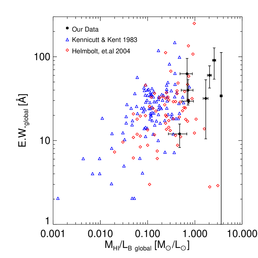
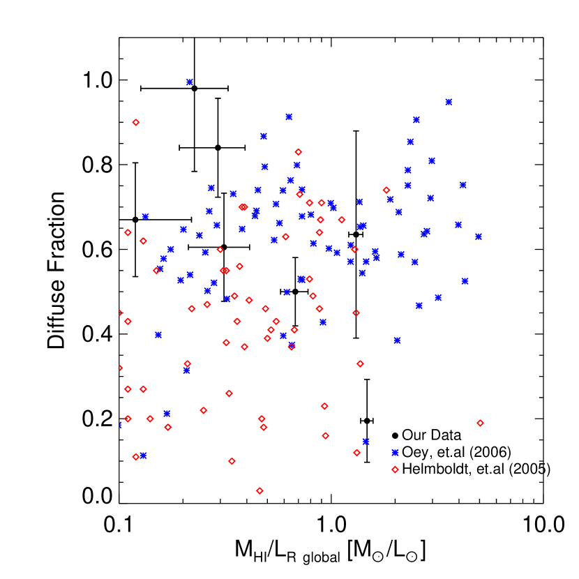
Figure 16: Gas mass to luminosity ratios plotted against global equivalent widths (left) and diffuse H$\alpha$ fractions (right). On the left, the (black) circles are our data, the (blue) triangles are from Kennicutt & Kent (1983) and the (red) diamonds are from Helmboldt, et al. (2004). On the right, the (black) circles are again our data, while the (blue) asterisks are from Oey, et al. (2006).

Figures 10 – 17 compare the properties of the H II regions and emission of our galaxy sample. Where possible, measurements from other samples of late-type galaxies are also shown (Kennicutt & Kent, 1983; Jansen, et al., 2000; Helmboldt, et al., 2005; Oey, et al., 2006). Examining the figures it is clear that the overall properties of our sample are similar to those of other late-type (Sbc-Sc) galaxies. That is, the values for the individual H II region luminosities are similar to those reported by Helmboldt, et al. (2005) and Kennicutt & Kent (1983) (Figure 10) while the global H$\alpha$ equivalent width (EW) and global star formation rates match those seen by all three comparison samples (Figures 11, 12).

We should note that as discussed in § 3 our sample suffers from having many of the H II regions blended together as a result of the distance to our galaxy samples. As a result, it is highly likely that in the comparisons of the luminosities for the galaxies’ individual H II regions the luminosities (Figure 10) from our sample are artificially higher then those in the other sample, potentially by a factor of 3 or more. This fact does not alter the results of this section, but it is the likely explanation for the slightly higher than average values found for L₃ in Figure 10.

To examine the total amount of gas found within the H II regions compared with that found in the diffuse H$\alpha$ gas, we need to determine the galaxies’ H$\alpha$ diffuse fraction, defined here as the ratio of H$\alpha$ flux not found within the defined H II regions to the total H$\alpha$ flux found for the entire galaxy. Examining Figures 13 and 14, as well as Tables 2 and 4, reveals an interesting fact – while the global SFR for these galaxies is fairly typical (0.3 – 5 M_⊙/yr), the combined SFR from the galaxies’ H II regions is a factor of 2 – 10 smaller. That is, on average the majority of the H$\alpha$ emission and thus the majority of the star formation in the observed galaxies comes not from the bright knots of star formation but instead from the galaxies’ diffuse H$\alpha$ gas. This is in contrast to the behavior seen from typical HSB galaxies, as evidenced by the data of Oey, et al. (2006) in Figure 13. We note that blending and angular resolution effects appear to be relatively unimportant in estimating the fraction of diffuse H$\alpha$ emission. Oey, et al. (2006) demonstrate this by showing no systematic changes in measured diffuse fractions as a function of distance up to almost 80 Mpc, and inclination angle, for their sample of 100+ SINGG survey galaxies.

While at first glance the higher diffuse H$\alpha$ fractions found for these galaxies seems surprising, recent GALEX results of the outer edges of M83, a region whose environment closely resembles that of the disks of massive LSB galaxies, also show considerable star formation outside the H II regions in that part of the galaxy (Thilker, et al., 2005). Similarly, Helmboldt, et al. (2005) found a slight trend with lower surface brightness galaxies having higher diffuse fractions than their higher surface brightness counterparts.

The fact that these galaxies have higher H$\alpha$ diffuse gas fractions raises an interesting question. Typically diffuse gas is believed to be ionized by OB stars lying within density-bounded H II regions. The problem of transporting the ionizing photons from these regions to the diffuse gas is extreme in these cases, as there would need to be a very large number of density-bound H II regions leaking ionizing photons to ionize the quantity of diffuse gas seen here. (See the more detailed discussion in Hoopes, Walterbos, & Bothun, 2001, which also discusses shock heating from stellar winds and SNe as ionization sources.) An alternative suggestion is that field OB stars are also ionizing the diffuse gas, as was suggested by Hoopes, Walterbos, & Bothun (2001). This would imply a different stellar population within and without the H II regions, as it would likely be the later OB types (B0–O9) which either escape the H II regions or survive the regions’ destruction. We note Oey, King, & Parker (2004) predict a modest increase in the fraction of field massive stars in galaxies with the lowest absolute star-formation rates. Scheduled GALEX observations of a subset of our observed galaxies may shed light on the underlying stellar population in the galaxies’ diffuse stellar disks.

Finally, it is elucidating to look for any trends between the global and regional properties of the galaxies and their SFR and H$\alpha$ content. Figure 15 plots the galaxies’ central surface brightness (in both B and R) against the galaxies’ total star formation rate. While the error bars make defining any trend difficult, there certainly appears to be a decrease in the global SFR with decreasing central surface brightness, similar to the trends seen in other studies (e.g. van den Hock, et al., 2000; Gerritsen & de Blok, 1999). Figure 16 shows the galaxies’ gas-to-luminosity ratios plotted against both their global equivalent width and diffuse H$\alpha$ fraction. In both cases, no trend can be seen with our data, although the small number of points available make any diagnosis difficult. Combined with the other datasets, though, we can see a general trend toward higher equivalent widths with increasing M_HI/L_B, but surprisingly no trend between gas fraction and the galaxies’ diffuse H$\alpha$ fraction is visible. This lack of correlation is also seen by Oey, et al. (2006). The last trend which can be seen is a rough correlation between the galaxies’ global color and star formation rate (Figure 11), with redder galaxies having higher SFR, a fact which may be a reddening effect. The individual H$\alpha$ regions, however, show no such trend (Figure 17).

7 Conclusion

The sample of 19 galaxies observed for this project were chosen to be large galaxies with low surface brightness disks. The surface brightness measurements for this sample were obtained originally through the UGC measurements through determining the galaxies’ average surface brightness within the $\mu$=25 mag arcsec^-2 isophote. The relation employed to determine the galaxies’ average surface brightness (Equation 7) has shown itself it be a good predictor of a galaxy’s central surface brightness. But for a wide variety of reasons the UGC measurements were not sufficient to insure the galaxies contained within this catalog have true LSB disks, underscoring the difficulty in designing targeted searches for large LSB galaxies.

Nonetheless, the sample of galaxies observed for this project have lower surface brightnesses than is found for a typical sample of large high surface brightness galaxies. In most other aspects the galaxies appear fairly ‘normal’, with colors typically B$-$R=0.3$-$0.9, morphological types ranging from Sb – Irr, and color gradients which typically grow bluer toward the outer radius. However, the galaxies have both higher gas mass-to-luminosity fractions and diffuse H$\alpha$ fractions than is found in higher surface brightness samples. This raises two questions. First, if the SFR for these galaxies has been similar to their higher surface brightness counterparts through the galaxies’ life, why do the lower surface brightness galaxies have higher gas mass-to-luminosity ratios? Second, why do these galaxies have a higher fraction of ionizing photons outside the density-bounded H II regions then their higher surface brightness counterparts?

The answer to the first question posed above likely comes from the difference between the studied galaxies’ current and historical SFR. As these galaxies have on average and lower metallicities (de Naray, McGaugh, & de Blok, 2004; Gerritsen & de Blok, 1999) than their higher surface brightness counterparts, it is likely that the galaxies’ SFR has not remained constant throughout the their lifetimes. Indeed the simplest explanation for the current similar SFRs and higher gas mass-to-luminosity ratios for the studied galaxies than for their higher surface brightness counterparts is that the galaxies’ past SFR was significantly different than is currently seen. In fact, the measured properties would be expected if the galaxies in this study have episodic star formation histories, with significant time (1-3 Gyr) lapsing between SF bursts, as has been conjectured for LSB galaxies in the past (e.g. Gerritsen & de Blok, 1999). Such a star formation history would help promote significant changes in the galaxies’ mean surface brightness and allow an individual large disk galaxy to appear as either (a) a relatively normal Hubble sequence spiral, (b) a large, lower surface brightness disk, or (c) perhaps even a lower surface brightness disk if the time between episodes is sufficiently large, depending on the elapsed time since the last SF burst. The final answer to this may be found when an answer to the second question, determining why the diffuse fractions for the studied galaxies is higher than for similar HSB galaxies, is also found. Irregardless, what is clear is that the studied sample shows a clear bridge between the known properties of high surface brightness galaxies and the more poorly understood properties of their very low surface brightness counterparts, such as Malin 1.

Table 1: Global Properties of Galaxies – B & R Measurements

					B					R
Galaxy	RA	Dec	Vel	Type	m	M	D25	$\langle\mu\rangle$		m	M	D25	$\langle\mu\rangle$	r	B$-$R	$i$
	$\left[J2000\right]$	$\left[J2000\right]$	$\left[km\;s^{-1}\right]$		$\left[mag\right]$	$\left[Mag\right]$	$\left[{}^{\prime\prime}\right]$	$\left[mag/\prime\prime^{2}\right]$		$\left[mag\right]$	$\left[Mag\right]$	$\left[{}^{\prime\prime}\right]$	$\left[mag/\prime\prime^{2}\right]$	$\left[{}^{\prime\prime}\right]$		$\left[{{}^{\circ}}\right]$
UGC 00023	00 04 13.0	10 47 25	7787	3	14.4 (0.1)	-20.7 (0.1)	71	23.4		13.0 (0.1)	-22.1 (0.1)	86.7	22.4	40	1.4 (0.2)	52
UGC 00189	00 19 57.5	15 05 32	7649	7	15.0 (0.2)	-20.1 (0.2)	84	24.4		13.8 (0.1)	-21.3 (0.1)	116.1	23.8	57	1.2 (0.2)	67
UGC 01362	01 52 50.7	14 45 52	7918	8.8	16.9 (0.2)	-18.2 (0.2)	30	24.3		15.6 (0.1)	-19.5 (0.1)	42.1	23.5	23	1.3 (0.3)	0
UGC 02299	02 49 07.8	11 07 09	10253	8	15.4 (0.2)	-20.3 (0.2)	59	24.0		14.5 (0.4)	-21.2 (0.4)	65.1	23.3	33	0.9 (0.4)	32
UGC 02588	03 12 26.5	14 24 27	10093	9.9	15.8 (0.2)	-19.9 (0.2)	39	23.6		14.7 (0.1)	-20.9 (0.1)	50.1	23.0	28	1.1 (0.2)	28
UGC 02796	03 36 52.5	13 24 24	9076	4	14.8 (0.2)	-20.6 (0.2)	66	23.6		13.3 (0.1)	-22.1 (0.1)	94.1	22.7	28	1.5 (0.2)	57
UGC 03119	04 39 07.7	11 31 50	7851	4	14.3 (0.2)	-20.8 (0.2)	71	23.7		12.4 (0.1)	-22.7 (0.1)		24.1	40	1.9 (0.2)	72
UGC 03308	05 26 01.8	08 57 25	8517	6	14.3 (0.3)	-21.0 (0.3)	89	23.8		14.0 (0.2)	-21.3 (0.2)	88.1	23.5	48	0.3 (0.4)	28
UGC 07598	12 28 30.9	32 32 52	9041	5.9	15.3 (0.1)	-20.1 (0.1)	46	23.5		14.8 (0.1)	-20.6 (0.1)	66.8	22.8	33	0.5 (0.2)	22
UGC 08311	13 13 50.8	23 15 16	3451	4.1	15.5 (0.1)	-17.9 (0.1)	50	23.8		14.8 (0.1)	-18.5 (0.1)	62.0	23.5	33	0.7 (0.2)	26
UGC 08644	13 40 01.4	07 22 00	6983	8	16.1 (0.2)	-18.8 (0.2)	43	24.2		15.3 (0.2)	-19.6 (0.2)	49.4	23.5	28	0.8 (0.3)	30
UGC 08904	13 58 51.1	26 06 24	9773	3.6	15.9 (0.1)	-19.7 (0.1)	43	23.8		14.9 (0.1)	-20.7 (0.1)	55.5	23.4	33	1.0 (0.2)	48
UGC 10894	17 33 03.8	27 34 29	6890	4	16.0 (0.3)	-18.8 (0.3)	48	24.1		14.9 (0.3)	-19.9 (0.3)		23.0	28	1.1 (0.4)	57
UGC 11068	17 58 05.0	28 14 38	4127	3.2	15.0 (0.2)	-18.7 (0.2)	64	24.0		13.8 (0.1)	-19.9 (0.1)	89.4	23.4	57	1.2 (0.2)	0
UGC 11355	18 47 57.0	22 56 33	4360	3.5	13.9 (0.3)	-19.9 (0.3)	173	24.8		12.5 (0.1)	-21.3 (0.1)		23.7	82	1.4 (0.3)	73
UGC 11396	19 03 49.5	24 21 28	4441	3.5	14.8 (0.3)	-19.1 (0.3)	114	24.4		13.8 (0.2)	-20.1 (0.2)	78.7	23.0	33	1.0 (0.4)	59
UGC 11617	20 43 39.3	14 17 52	5119	6.1	14.9 (0.2)	-19.2 (0.2)	75	24.1		13.9 (0.2)	-20.3 (0.2)	86.1	23.3	40	1.1 (0.3)	58
UGC 11840	21 53 18.0	04 14 50	7986	4	16.3 (0.1)	-18.9 (0.1)	24	22.9		15.3 (0.1)	-19.9 (0.1)	23.3	21.9	11	1.0 (0.2)	40
UGC 12021	22 24 11.6	06 00 12	4472	3	14.7 (0.2)	-19.2 (0.2)	113	24.7		13.6 (0.1)	-20.2 (0.1)	130.4	23.9	57	1.1 (0.2)	63

Note. — Errors are given in parenthesis.

Table 2: Global Properties of Galaxies – H$\alpha$

Galaxy	H$\alpha$ flux $\times 10^{-13}$	EW	SFR	r
	$\left[erg\;cm^{-2}\;s^{-1}\right]$	$\rm\left[\AA\right]$	$\rm\left[{M_{\odot}yr^{-1}}\right]$	$\rm\left[{}^{\prime\prime}\right]$
UGC 00023	5 (1)	22 (8)	4 (1)	28
UGC 00189	4 (1)	63 (33)	4 (1)	23
UGC 01362	$\cdots$	$\cdots$	$\cdots$	$\cdots$
UGC 02299	0.41 (0.09)	38 (13)	0.7 (0.2)	6
UGC 02588	0.7 (0.3)	32 (21)	1.1 (0.5)	13
UGC 02796	2.1 (0.7)	12 (4)	2.7 (0.9)	13
UGC 03119	7 (4)	20 (12)	6 (6)	28
UGC 03308	1.0 (0.3)	22 (8)	1.1 (0.3)	11
UGC 07598	1.3 (0.3)	60. (18)	1.8 (0.4)	19
UGC 08311	3.1 (0.6)	91 (37)	0.6 (0.1)	19
UGC 08644	$\cdots$	$\cdots$	$\cdots$	$\cdots$
UGC 08904	0.8 (0.2)	40 (13)	1.1 (0.3)	16
UGC 10894	0.4 (1)	34 (78)	0.4 (0.1)	9
UGC 11068	$\cdots$	$\cdots$	$\cdots$	$\cdots$
UGC 11355	8 (2)	30 (9)	2.7 (0.6)	28
UGC 11396	2.4 (0.8)	400 (2000)	0.8 (0.2)	16
UGC 11617	3.1 (0.7)	30 (2)	0.3 (0.2)	19
UGC 11840	$\cdots$	$\cdots$	$\cdots$	$\cdots$
UGC 12021	4 (1)	63 (32)	1.3 (0.4)	23
UGC 12289	$\cdots$	$\cdots$	$\cdots$	$\cdots$

Note. — Derivation of quantities are described in Section 3. Errors are given in parenthesis.

Table 3: Fitted Galaxy Properties

			inner			outer
Galaxy	Fit	Filter	$\mu_{eff}/\mu_{0}$	$R_{eff}/\alpha$		$\mu_{0}$	$\alpha$	Boundary	Fit
	Type		$\left[mag\;arcsec^{-2}\right]$	$\left[{}^{\prime\prime}\right]$		$\left[mag\;arcsec^{-2}\right]$	$\left[{}^{\prime\prime}\right]$	$\left[{}^{\prime\prime}\right]$	Error
UGC 00023	Two Disk	B	19.06 (0.33)	1.71 (0.02)		21.17 (0.21)	11.05 (0.06)	6.55	0.82
UGC 00023	Two Disk	R	17.30 (0.27)	1.72 (0.02)		19.58 (0.16)	9.58 (0.03)	6.93	0.53
UGC 00023	Bulge/Disk	B	21.48 (1.98)	4.06 (0.23)		21.47 (0.51)	11.96 (0.11)	8.94	0.89
UGC 00023	Bulge/Disk	R	19.20 (1.56)	3.07 (0.14)		19.82 (0.35)	9.96 (0.05)	8.79	0.58
UGC 00189	Two Disk	B	20.99 (0.08)	7.75 (0.06)		24.05 (1.85)	36.90 (2.11)	28.34	0.33
UGC 00189	Two Disk	R	19.53 (0.09)	6.13 (0.05)		21.66 (0.67)	18.84 (0.22)	24.92	0.97
UGC 01362	One Disk	B	$\cdots$	$\cdots$		23.06 (0.33)	7.77 (0.10)	$\cdots$	1.78
UGC 01362	One Disk	R	$\cdots$	$\cdots$		21.84 (0.15)	7.85 (0.04)	$\cdots$	0.46
UGC 02299	Two Disk	B	20.85 (0.10)	2.00 (0.16)		22.43 (1.76)	11.24 (0.04)	6.48	1.88
UGC 02299	Two Disk	R	19.84 (0.28)	2.21 (0.03)		21.46 (0.38)	10.50 (0.10)	7.23	0.99
UGC 02299	Bulge/Disk	B	25.10 (2.85)	17.35 (1.95)		23.23 (2.18)	12.62 (0.27)	17.01	2.08
UGC 02299	Bulge/Disk	R	24.00 (1.75)	17.76 (1.24)		22.30 (1.43)	10.37 (0.19)	0.00	1.18
UGC 02588	One Disk	B	$\cdots$	$\cdots$		21.50 (0.08)	5.47 (0.02)	$\cdots$	1.40
UGC 02588	One Disk	R	$\cdots$	$\cdots$		20.41 (0.07)	5.79 (0.02)	$\cdots$	1.12
UGC 02588	Bulge/Disk	B	25.75 (2.43)	16.16 (1.75)		22.61 (0.97)	8.78 (0.08)	6.94	1.18
UGC 02588	Bulge/Disk	R	23.77 (2.50)	7.86 (0.75)		21.09 (0.48)	7.41 (0.04)	4.57	0.82
UGC 02796	Two Disk	B	19.07 (0.34)	1.89 (0.03)		21.02 (0.60)	8.75 (0.14)	6.90	0.48
UGC 02796	Two Disk	R	17.52 (0.27)	2.19 (0.03)		19.66 (0.41)	8.69 (0.08)	8.59	0.68
UGC 02796	Bulge/Disk	B	23.07 (2.01)	13.80 (1.10)		22.54 (4.11)	8.92 (0.45)		0.71
UGC 02796	Bulge/Disk	R	21.01 (0.90)	10.26 (0.31)		20.49 (1.06)	6.76 (0.22)		0.21
UGC 03119	One Disk	B	$\cdots$	$\cdots$		19.82 (0.07)	10.35 (0.03)	$\cdots$	0.75
UGC 03119	One Disk	R	$\cdots$	$\cdots$		17.92 (0.05)	9.48 (0.01)	$\cdots$	0.49
UGC 03119	Bulge/Disk	B	22.05 (9.17)	3.54 (0.91)		20.03 (0.31)	11.51 (0.08)	3.50	0.61
UGC 03119	Bulge/Disk	R	21.07 (5.81)	6.53 (1.29)		18.16 (0.24)	10.10 (0.02)	3.71	0.28
UGC 03308	Two Disk	B	19.83 (2.25)	0.87 (0.04)		21.70 (0.18)	15.47 (0.16)	3.47	0.35
UGC 03308	Two Disk	R	19.06 (1.32)	0.92 (0.03)		20.99 (0.13)	11.60 (0.06)	3.58	0.25
UGC 03308	Bulge/Disk	B	18.36 (10.1)	0.43 (0.08)		21.71 (0.23)	15.66 (0.18)	3.62	0.37
UGC 03308	Bulge/Disk	R	18.70 (5.77)	0.67 (0.08)		21.03 (0.18)	11.90 (0.08)	3.85	0.20
UGC 07598	One Disk	B	$\cdots$	$\cdots$		21.69 (0.07)	7.96 (0.02)	$\cdots$	0.75
UGC 07598	One Disk	R	$\cdots$	$\cdots$		19.82 (0.08)	6.26 (0.02)	$\cdots$	1.12
UGC 07598	Bulge/Disk	B	16.02 (6.98)	0.21 (0.03)		21.84 (0.13)	8.60 (0.03)	3.25	0.52
UGC 07598	Bulge/Disk	R	15.78 (3.90)	0.40 (0.03)		20.18 (0.21)	7.34 (0.04)	4.06	0.49
UGC 08311	Two Disk	B	20.82 (0.09)	2.94 (0.02)		23.29 (0.66)	14.91 (0.26)	12.50	0.48
UGC 08311	Two Disk	R	20.28 (0.08)	3.22 (0.03)		22.73 (0.71)	15.81 (0.32)	13.64	0.39
UGC 08644	One Disk	B	$\cdots$	$\cdots$		22.56 (0.14)	8.79 (0.06)	$\cdots$	0.55
UGC 08644	One Disk	R	$\cdots$	$\cdots$		21.19 (0.15)	6.40 (0.04)	$\cdots$	0.78
UGC 08904	Two Disk	B	20.43 (0.16)	2.56 (0.02)		22.94 (0.71)	10.07 (0.15)	11.22	0.69
UGC 08904	Two Disk	R	18.90 (0.16)	2.20 (0.01)		22.05 (0.49)	9.67 (0.10)	11.19	0.35
UGC 08904	Bulge Only	B	23.99 (0.27)	12.55 (0.09)		$\cdots$	$\cdots$	$\cdots$	1.17
UGC 08904	Bulge Only	R	21.83 (0.25)	6.95 (0.04)		$\cdots$	$\cdots$	$\cdots$	0.48
UGC 10894	One Disk	B	$\cdots$	$\cdots$		21.65 (0.10)	7.90 (0.04)	$\cdots$	0.44
UGC 10894	One Disk	R	$\cdots$	$\cdots$		20.26 (0.12)	6.69 (0.04)	$\cdots$	0.42
UGC 11068	Two Disk	B	20.15 (0.65)	1.15 (0.02)		22.46 (0.13)	13.65 (0.07)	4.87	0.31
UGC 11068	Two Disk	R	18.67 (0.54)	1.25 (0.02)		21.02 (0.14)	11.26 (0.05)	5.23	0.54
UGC 11068	Bulge/Disk	B	20.36 (0.18)	1.00 (0.00)		22.53 (0.11)	14.10 (0.06)	5.31	0.38
UGC 11068	Bulge/Disk	R	19.89 (2.52)	1.66 (0.10)		21.18 (0.25)	11.97 (0.07)	6.23	0.42
UGC 11355	Two Disk	B	19.20 (0.15)	3.34 (0.02)		21.61 (0.18)	32.30 (0.24)	14.23	0.86
UGC 11355	Two Disk	R	17.30 (0.16)	3.01 (0.02)		19.83 (0.13)	24.07 (0.10)	13.02	0.64
UGC 11355	Bulge/Disk	B	23.29 (0.95)	19.99 (0.72)		22.13 (0.56)	38.81 (0.57)	26.27	1.13
UGC 11355	Bulge/Disk	R	20.70 (0.94)	10.96 (0.37)		20.19 (0.35)	26.30 (0.18)	26.30	0.93
UGC 11396	Two Disk	B	20.34 (1.82)	1.14 (0.05)		22.08 (0.27)	22.66 (0.39)	4.46	0.95
UGC 11396	Two Disk	R	19.77 (2.17)	1.23 (0.08)		20.20 (0.17)	13.04 (0.10)	2.80	1.69
UGC 11396	Bulge/Disk	B	20.52 (9.40)	0.97 (0.19)		22.10 (0.35)	23.03 (0.45)	4.75	0.93
UGC 11396	Bulge/Disk	R	20.09 (3.23)	1.09 (0.32)		20.21 (0.23)	13.03 (0.11)	3.03	1.69
UGC 11617	One Disk	B	$\cdots$	$\cdots$		21.30 (0.07)	12.83 (0.05)	$\cdots$	0.69
UGC 11617	One Disk	R	$\cdots$	$\cdots$		20.08 (0.08)	10.99 (0.04)	$\cdots$	0.46
UGC 11840	No Fit	B	$\cdots$	$\cdots$		$\cdots$	$\cdots$	$\cdots$	$\cdots$
UGC 11840	No Fit	R	$\cdots$	$\cdots$		$\cdots$	$\cdots$	$\cdots$	$\cdots$
UGC 12021	One Disk	B	$\cdots$	$\cdots$		20.73 (0.06)	11.05 (0.02)	$\cdots$	1.63
UGC 12021	One Disk	R	$\cdots$	$\cdots$		19.41 (0.06)	10.26 (0.02)	$\cdots$	1.58
UGC 12021	Bulge/Disk	B	26.49 (1.28)	23.19 (0.00)		20.88 (0.16)	11.59 (0.04)	2.37	1.54
UGC 12021	Bulge/Disk	R	23.85 (0.32)	23.19 (0.00)		19.96 (0.18)	11.60 (0.03)	6.23	1.01

Note. — Derivation of quantities is described in Section 3. Errors are given in parenthesis.

Table 4: Properties of H$\alpha$ Regions

Galaxy	Region	H$\alpha$ Flux $\times 10^{-15}$	H$\alpha$ Luminosity$\times 10^{38}$	SFR	EW	B	R	B$-$R	Diffuse
		$\left[erg\;cm^{-2}\;s^{-1}\right]$	$\left[erg\;s^{-1}\right]$	$\left[M_{\odot}\;yr^{-1}\right]$	$\rm\left[\AA\right]$	$\left[mag\right]$	$\left[mag\right]$	$\left[mag\right]$	$\left[\%\right]$
UGC 00023	1	70 (14)	760 (150)	0.6 (0.1)	23 (1)	16.9 (0.1)	15.2 (0.1)	1.7 (0.2)	0.82 (0.04)
UGC 00189	1	10 (2)	110 (20)	0.09 (0.02)	30 (2)	19.9 (0.6)	18.3 (0.5)	1.7 (0.7)	0.98 (0.01)
UGC 01362	0	$\cdots$	$\cdots$	$\cdots$	$\cdots$	$\cdots$	$\cdots$	$\cdots$	$\cdots$
UGC 02299	1	12 (2)	240 (50)	0.19 (0.04)	20 (1)	21 (2)	21 (2)	0. (3)	$\cdots$
UGC 02299	2	15 (3)	260 (50)	0.21 (0.04)	14 (1)	18.2 (0.2)	17.1 (0.2)	1.1 (0.3)	$\cdots$
UGC 02299	TOTAL	22 (3)	490 (70)	0.39 (0.06)	$\cdots$	$\cdots$	$\cdots$	$\cdots$	0.45 (0.06)
UGC 02588	0	$\cdots$	$\cdots$	$\cdots$	$\cdots$	$\cdots$	$\cdots$	$\cdots$	$\cdots$
UGC 02796	1	74.8 (15)	900 (200)	0.71 (0.1)	10 (1)	16.5 (0.2)	14.8 (0.4)	1.7 (0.4)	0.67 (0.01)
UGC 03119	1	151 (30)	1600 (300)	1.3 (0.3)	16 (1)	18.8 (0.1)	16.7 (0.1)	2 (0.1)	0.77 (0.02)
UGC 03308	0	$\cdots$	$\cdots$	$\cdots$	$\cdots$	$\cdots$	$\cdots$	$\cdots$	$\cdots$
UGC 07598	1	6 (1)	80 (17)	0.07 (0.01)	13 (1)	22.2 (0.7)	21.5 (0.7)	0.6 (1)	$\cdots$
UGC 07598	2	4.7 (0.9)	60 (12)	0.05 (0.01)	12 (1)	22 (1)	20.2 (0.9)	2 (1)	$\cdots$
UGC 07598	3	2.4 (0.5)	32 (6)	0.03 (0.01)	13 (1)	23 (1)	21 (1)	2 (2)	$\cdots$
UGC 07598	4	6 (1)	80 (20)	0.06 (0.01)	12 (1)	21.1 (0.8)	19.6 (0.7)	2 (1)	$\cdots$
UGC 07598	5	3.3 (0.7)	43 (9)	0.03 (0.01)	13 (1)	23 (2)	22 (2)	2 (3)	$\cdots$
UGC 07598	6	6 (1)	80 (20)	0.06 (0.01)	11 (1)	21 (3)	22 (3)	-1 (4)	$\cdots$
UGC 07598	7	4.1 (0.8)	50 (10)	0.04 (0.01)	11 (1)	22 (1)	21 (2)	1 (4)	$\cdots$
UGC 07598	8	1.3 (0.3)	15 (3)	0.012 (0.003)	9 (1)	25 (3)	24 (3)	1 (3)	$\cdots$
UGC 07598	9	32 (6)	430 (90)	0.34 (0.07)	13 (1)	18 (0.1)	16 (0.1)	1.9 (3)	$\cdots$
UGC 07598	10	1.4 (0.3)	20. (4)	0.015 (0.003)	16 (1)	21.8 (0.5)	20.4 (0.5)	1.3 (0.5)	$\cdots$
UGC 07598	11	10 (2)	130 (30)	0.11 (0.02)	11 (1)	21.4 (0.5)	20 (0.6)	1.4 (0.8)	$\cdots$
UGC 07598	12	4.8 (1)	60 (10)	0.05 (0.01)	11 (1)	22 (1)	20.2 (0.9)	2 (1)	$\cdots$
UGC 07598	13	4.4 (0.9)	60 (10)	0.05 (0.01)	12 (1)	21.8 (0.8)	20.1 (0.7)	2 (1)	$\cdots$
UGC 07598	14	5 (1)	70 (10)	0.05 (0.01)	11 (1)	22.7 (1)	21 (1)	1 (2)	$\cdots$
UGC 07598	TOTAL	69 (6)	1200 (100)	0.96 (0.08)	$\cdots$	$\cdots$	$\cdots$	$\cdots$	0.5 (0.1)
UGC 08311	1	7 (1)	14 (3)	0.011 (0.002)	20. (1)	21.3 (0.7)	21 (0.9)	0. (1)	$\cdots$
UGC 08311	2	100 (20)	240 (50)	0.19 (0.04)	53 (1)	18.8 (0.4)	18.4 (0.5)	0.3 (0.6)	$\cdots$
UGC 08311	3	7 (1)	16 (3)	0.012 (0.003)	18 (1)	20.8 (0.1)	20. (1)	1 (1)	$\cdots$
UGC 08311	4	17 (3)	38 (8)	0.03 (0.01)	29 (1)	0.9 (0.1)	20.5 (0.9)	-19.6 (0.9)	$\cdots$
UGC 08311	5	8 (2)	18 (4)	0.015 (0.003)	25 (1)	22 (2)	22 (2)	1 (3)	$\cdots$
UGC 08311	6	140 (30)	320 (60)	0.26 (0.05)	38 (1)	16.9 (0.1)	16.3 (0.1)	0.6 (0.1)	$\cdots$
UGC 08311	7	15 (3)	32 (6)	0.03 (0.01)	19 (1)	18.6 (0.1)	18.1 (0.2)	0.6 (0.2)	$\cdots$
UGC 08311	TOTAL	270 (30)	680 (80)	0.54 (0.07)	$\cdots$	$\cdots$	$\cdots$	$\cdots$	0.2 (0.1)
UGC 08644	1	5.1 (1)	44 (9)	0.04 (0.01)	17 (1)	21 (0.1)	20. (1)	1 (1)	$\cdots$
UGC 08644	2	4.8 (1)	42 (8)	0.03 (0.01)	20. (1)	22 (0.5)	21.1 (0.6)	0.9 (0.8)	$\cdots$
UGC 08644	TOTAL	8.3 (1)	90 (10)	0.07 (0.01)	$\cdots$	$\cdots$	$\cdots$	$\cdots$	$\cdots$
UGC 08904	1	3.4 (0.7)	47 (9)	0.04 (0.01)	10. (1)	22.4 (0.8)	22 (1)	1 (1)	$\cdots$
UGC 08904	2	0.7 (0.1)	12 (2)	0.01 (0.009)	23 (1)	23.6 (0.5)	23.0 (0.6)	0.7 (0.8)	$\cdots$
UGC 08904	3	1.2 (0.3)	20. (4)	0.02 (0.02)	16 (1)	24.3 (0.7)	24 (1)	1 (1)	$\cdots$
UGC 08904	4	0.8 (0.2)	12 (2)	0.01 (0.009)	10. (1)	23.8 (0.4)	24 (1)	0. (1)	$\cdots$
UGC 08904	5	0.7 (0.1)	9 (2)	0.01 (0.007)	10. (1)	24.5 (0.9)	24 (1)	1 (2)	$\cdots$
UGC 08904	6	32 (6)	600 (100)	0.45 (0.09)	25 (1)	17.7 (0.1)	16.3 (0.1)	1.4 (0.1)	$\cdots$
UGC 08904	TOTAL	33 (6)	700 (100)	0.53 (0.09)	$\cdots$	$\cdots$	$\cdots$	$\cdots$	0.6 (0.1)
UGC 10894	1	1.2 (0.2)	11 (2)	0.009 (0.002)	39 (3)	24 (2)	23 (1)	1 (2)	$\cdots$
UGC 10894	2	1.4 (0.3)	13 (3)	0.010 (0.002)	37 (2)	22.1 (0.5)	21.3 (0.6)	0.8 (0.8)	$\cdots$
UGC 10894	3	13 (3)	110 (20)	0.09 (0.02)	27 (1)	18.9 (0.2)	17.2 (0.1)	1.8 (0.2)	$\cdots$
UGC 10894	4	1.9 (0.4)	18 (4)	0.014 (0.003)	31 (2)	23 (1)	22 (1)	1 (2)	$\cdots$
UGC 10894	5	1.8 (0.4)	16 (3)	0.013 (0.003)	35 (2)	22.8 (0.7)	21.9 (0.7)	1 (1)	$\cdots$
UGC 10894	6	2.8 (0.6)	26 (5)	0.020 (0.004)	36 (2)	22.4 (0.7)	22 (1)	0. (1)	$\cdots$
UGC 10894	7	3.9 (0.8)	35 (7)	0.03 (0.01)	31 (2)	22.6 (0.8)	21.6 (0.8)	1 (1)	$\cdots$
UGC 10894	TOTAL	23 (2)	230 (25)	0.18 (0.02)	$\cdots$	$\cdots$	$\cdots$	$\cdots$	0.6 (0.3)
UGC 11068	0	$\cdots$	$\cdots$	$\cdots$	$\cdots$	$\cdots$	$\cdots$	$\cdots$	$\cdots$
UGC 11355	1	180 (40)	600 (100)	0.48 (0.1)	17 (1)	19.7 (0.4)	18.2 (0.4)	1.5 (0.6)	0.87 (0.08)
UGC 11396	1	25 (5)	90 (20)	0.07 (0.01)	21 (1)	22 (1)	18.1 (0.2)	4 (1)	0.91 (0.01)
UGC 11617	1	9 (2)	40 (8)	0.07 (0.01)	12 (1)	21 (1)	21 (0.6)	0. (1)	$\cdots$
UGC 11617	2	21 (4)	90 (20)	0.04 (0.01)	13 (1)	21 (2)	20. (2)	1 (3)	$\cdots$
UGC 11617	3	13 (3)	50 (10)	0.04 (0.01)	13 (1)	22 (2)	20. (3)	1 (3)	$\cdots$
UGC 11617	4	12 (2)	47 (9)	0.09 (0.01)	11 (1)	21 (2)	21 (1)	1 (3)	$\cdots$
UGC 11617	5	26 (5)	110 (20)	0.03 (0.02)	14 (1)	21.5 (0.6)	21 (4)	1 (4)	$\cdots$
UGC 11617	6	10 (2)	42 (8)	0.03 (0.01)	12 (1)	21.5 (0.2)	20.8 (0.7)	0.7 (0.7)	$\cdots$
UGC 11617	TOTAL	69 (6)	390 (30)	0.31 (0.03)	$\cdots$	$\cdots$	$\cdots$	$\cdots$	0.8 (0.1)
UGC 11840	0	$\cdots$	$\cdots$	$\cdots$	$\cdots$	$\cdots$	$\cdots$	$\cdots$	$\cdots$
UGC 12021	1	13 (3)	50 (10)	0.04 (0.01)	31 (2)	19.2 (0.4)	17.8 (0.3)	1.4 (0.5)	0.97 (0.01)

Note. — Derivation of quantities is described in Section 3. Errors are given in parenthesis.

Figure 1: Grey scale images of the observed galaxies. Figure available through the published AJ paper or online at http://www.gb.nrao.edu/$\sim$koneil.

Figure 2: Surface brightness profiles for all galaxies observed. The dash-dotted lines show the inner fit, the dashed lines show the outer fit, and the solid lines show the combined fits. Both the B (blue - bottom) and R (red - top) profiles are shown. Figure available through the published AJ paper or online at http://www.gb.nrao.edu/$\sim$koneil.

Figure 3: Color profiles for all the galaxies observed. Here the inner fits (when made) are shown by a dashed line and the outer fits are shown by a solid line. Figure available through the published AJ paper or online at http://www.gb.nrao.edu/$\sim$koneil.

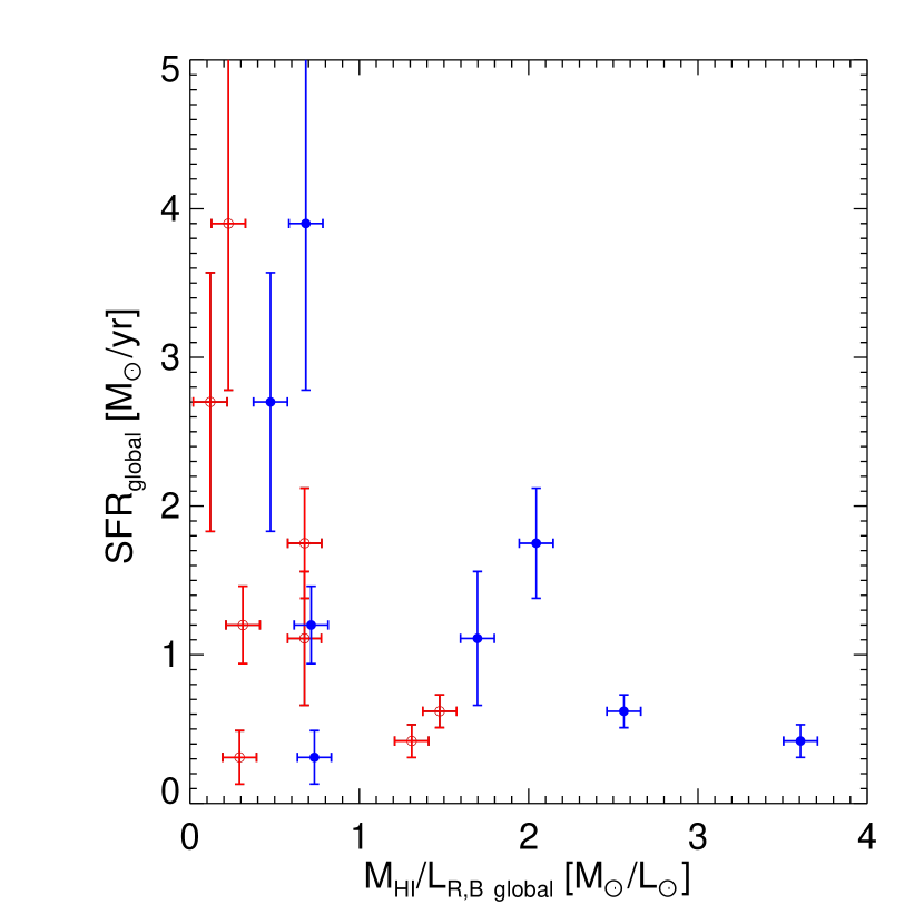
Figure 9: Gas mass to B and R-band luminosity ratios plotted against the global star formation rate for the galaxies. The (blue) filled circles are for the B-band data and the (red) open circles are for the R-band data.

Figure 17: This plot shows the regional colors versus star formation rates for the observed galaxies.

References

- Bothun & Cornell (1990) Bothun, G. D. & Cornell, M. 1990 AJ 99, 1004
- Bothun, et al. (1986) Bothun, G. D., Beers, T. C., Mould, J. R., & Huchra, J. P. 1986 ApJ 308, 510
- Bothun, et al. (1985) Bothun, G. D., Beers, T. C., Mould, J. R., & Huchra, J. P. 1985 AJ 90 2487
- Bottinelli, et al. (1995) Bottinelli, L., Gouguenheim, L., Paturel, G., Teerikorpi, P. 1995 A&A 296, 64
- Broeils & Courteau (1997) Broeils, A. H. & Courteau, S. 1997 ASPC 117, 74
- Cornell, et al. (1987) Cornell, M., Aaronson, M., Bothun, G., & Mould, J. 1987 ApJS 64, 507
- Das, et al. (2006) Das, M., O’Neil, K., Vogel, S., & McGaugh, S. 2006 ApJ preprint
- de Jong (1996) de Jong, R. S. 1996 A&AS 118, 557
- de Naray, McGaugh, & de Blok (2004) de Naray, Rachel Kuzio, McGaugh, Stacy S., & de Blok, W. J. G. 2004 MNRAS 355, 887
- de Vaucouleurs, et al. (1991) de Vaucouleurs, G, de Vaucouleurs, Antoinette, Corwin, Herold G., Jr., Buta, Ronald J., Paturel, Georges, & Fouque, Pascal Third Reference Catalogue of Bright Galaxies 1991 Springer-Verlag Berlin Heidelberg New York
- Fouqué & Paturel (1985) Fouqué, P. & Paturel, G.(1985) A&A 150, 192
- Freeman (1970) Freeman, K. 1970 ApJ 160, 811
- Gavazzi, et al. (2006) Gavazzi, G., Boselli, A., Cortese, L., Arosio, I., Gallazzi, A., Pedotti, P., & Carrasco, L. 2006 A&A 446, 839
- Gerritsen & de Blok (1999) Gerritsen, Jeroen P. E. & de Blok, W. J. G. 1999 A&A 342, 655
- Gurovich, et al. (2004) Gurovich, Sebasti n, McGaugh, Stacy S., Freeman, Ken C., Jerjen, Helmut, Staveley-Smith, Lister, & de Blok, W. J. G. 2004 PASA 21, 412
- Helmboldt, et al. (2005) Helmboldt, J.F., Walterbos, R.A.M., Bothun, G.D., O’Neil, K. 2005, ApJ, 630, 824
- Helmboldt, et al. (2004) Helmboldt, J.F., Walterbos, R.A.M., Bothun, G.D., O’Neil, K., de Blok, W.J.G. 2004 ApJ, 613, 914
- Hodge & Kennicutt (1983) Hodge, P. W. & Kennicutt, R. C. Jr. 1983 ApJ 267, 563
- Hoopes, Walterbos, & Bothun (2001) Hoopes, Charles G., Walterbos, Ren A. M., & Bothun, Gregory D. 2001 ApJ 559, 878
- Howarth (1983) Howarth, I 1983 MNRAS 203, 301
- Impey & Bothun (1997) Impey, C. & Bothun, G.D. 1997 ARA&A 35, 267
- Jansen, et al. (2000) Jansen, R., Fabricant, D., Franx, M., Caldwell, N. 2000 ApJS 126, 331
- Kennicutt, et al. (2004) Kennicutt, W.C. Jr, Lee, J. C., Akiyama, S., Funes, J. G., & Sakai, S. 2004 AAS 205, 6005
- Kennicutt (1998) Kennicutt, W.C. Jr 1998 ARA&A 36, 189
- Kennicutt, Tamblyn, & Congdon (1994) Kennicutt, W.C. Jr, Tamblyn, P., & Congdon, C. 1994 ApJ 435, 22
- Kennicutt & Kent (1983) Kennicutt, R. C. Jr & Kent 1983 AJ 88 1094
- Kennicutt (1983) Kennicutt, R. C. Jr 1983 ApJ 272, 54
- Koopman & Kenney (2006) Koopman, E. & Kenney, J. 2006 ApJS 162, 97
- McCall, Rybski, & Shields (1985) McCall, M. L., Rybski, P. M., & Shields, G. A. 1985 ApJS 57, 1
- McGaugh, Rubin, & de Blok (2001) McGaugh, Stacy S., Rubin, Vera C., & de Blok, W. J. G 2001 AJ 122, 2381
- McGaugh, et al. (2000) McGaugh, S. S., Schombert, J. M., Bothun, G. D., & de Blok, W. J. G. 2000, ApJ 533, L99
- Meurer, et al. (2006) Meurer, G., Hanish, D.J., Ferguson, H.C., Knezek, P., et al.2006 ApJS 165, 307
- Nilson (1973) Nilson, P. Uppsala General Catalogue of Galaxies (UGC) Acta Universitatis Upsalienis, Nova Regiae Societatis Upsaliensis, Series
- O’Donnell (1994) O’Donnell, J 1994 ApJ 437, 262
- Oey, et al. (2006) Oey, et al.2006 - preprint
- Oey, King, & Parker (2004) Oey, M. S., King, N. L., & Parker, J. W. 2004, AJ 127, 1632
- Oey & Kennicutt (1993) Oey, S. & Kennicutt, R. 1993 ApJ 411, 137O
- O’Neil, van Driel, & Schneider (2006) O’Neil, K. van Driel, W. & Schneider, S. 2006 in preparation
- O’Neil, et al. (2004) O’Neil, K., Bothun, G., van Driel, W., & Monnier-Ragaigne, D. 2004 A&A 428, 823
- O’Neil & Schinnerer (2004) O’Neil, K. & Schinnerer, E. 2004 ApJ 615, L109
- O’Neil, Schinnerer, & Hofner (2003) O’Neil, K., Schinnerer, E., & Hofner, P. 2003 ApJ 588, 230
- O’Neil, Bothun, & Schombert (2000) O’Neil, K., Bothun, G., Schombert, J. 2000 AJ 119. 136
- O’Neil, Hofner, & Schinnerer (2000) O’Neil, K., Hofner, P., & Schinnerer, E. 2000 ApJ 545, L99
- Osterbrock (1989) Osterbrock, D. 1989 Astrophysics of Gaseous Nebulae and Active Galactic Nuclei University Science Books
- Pickering, et al. (1997) Pickering, T. E., Impey, C. D., van Gorkom, J. H., & Bothun, G. D. 1997 AJ 114, 1858
- Roennback & Bergvall (1995) Roennback, J., & Bergvall, N. 1995 A&A 302, 353
- Schombert & Bothun (1988) Schombert, J. & Bothun, G. 1988 AJ 91, 1389
- Seaton (1979) Seaton, M. 1979 MNRAS 187, 73
- Simien & de Vaucouleurs (1986) Simien, F. & de Vaucouleurs, G. 1986 ApJ 302, 564
- Sprayberry, et al. (1995) Sprayberry, D., Impey, C. D., Bothun, G. D. & Irwin, M. J. 1995 AJ 109, 558
- Thilker, et al. (2005) Thilker, D., et al.2005 ApJ 619L, 79
- Thilker, Braun, & Walterbos (2000) Thilker, David A., Braun, Robert, & Walterbos, Ren A. M. 2000 AJ 120 3070
- Tully, et al. (1998) Tully, R. Brent, Pierce, Michael J., Huang, Jia-Sheng, Saunders, Will, Verheijen, Marc A. W., & Witchalls, Peter L. 1998 AJ 115, 2264
- Tully & Fouqué (1985) Tully, B. & Fouqué 1985 ApJS 58, 67
- Tully & Fisher (1977) Tully, B. & Fisher, R. 1977 A&A 54, 661
- van den Hock, et al. (2000) van den Hoek, L. B., de Blok, W. J. G., van der Hulst, J. M., & de Jong, T. 2000 A&A 357, 397
- Verheijen (1997) Verheijen, M. 1997 Ph.D. Dissertation Kapteyn Institute, Groningen
- Zwaan, et al. (1995) Zwaan, M.A., van der Hulst, J.M., de Blok, W.J.G., & McGaugh, S.S. 1995 MNRAS 273, L35