Domain Wall Dynamics near a Quantum Critical Point

Abstract

We study the real-time domain-wall dynamics near a quantum critical point of the one-dimensional anisotropic ferromagnetic spin $1/2$ chain. By numerical simulation, we find the domain wall is dynamically stable in the Heisenberg-Ising model. Near the quantum critical point, the width of the domain wall diverges as $\left(\Delta-1\right)^{-1/2}$.

year number number identifier

I Introduction

Recent progress in synthesizing materials that contain ferromagnetic chainsKaji05 ; Mito05 ; Kage97 ; Maig00 provides new opportunities to study the quantum dynamics of atomic-size domain walls (DW). On the atomic level, a DW is a structure that is stable with respect to (quantum) fluctuations, separating two regions with opposite magnetization. Such a structure was observed in the one-dimensional CoCl${}_{2}\cdot 2$H₂O chainTorrance69 ; Nicoli74 .

In an earlier paperYuan06 , we studied the propagation of spin waves in ferromagnetic quantum spin chains that support DWs. We demonstrated that DWs are very stable against perturbations, and that the longitudinal component of the spin wave speeds up when it passes through a DW while the transverse component is almost completely reflected.

In this paper, we focus on the dynamic stability of the DW in the Heisenberg-Ising ferromagnetic chain. It is known that the ground state of this model in the subspace of total magnetization zero supports DW structuresGochev77 ; Gochev83 . However, if we let the system evolve in time from an initial state with a DW structure and this initial state is not an eigenstate, it must contain some excited states. Therefore, the question whether the DW structure will survive in the stationary (long-time) regime is nontrivial.

The question how the DW structure dynamically survives in the stationary (long-time) region is an interesting problem. In particular, we focus on the stability of the DW with respect to the dynamical (quantum) fluctuations as we approach the quantum critical point (from Heisenberg-Ising like to Heisenberg). We show that the critical quantum dynamics of DWs can be described well in terms of conventional power laws. The behavior of quantum systems at or near a quantum critical point is of contemporary interestSachdev99 . We also show that the DW profiles rapidly become very stable as we move away from the quantum critical point.

II Model

The Hamiltonian of the system is given byMIKE91 ; Cloizeaux66 ; Gochev77 ; Gochev83 ; MATT81

$$H=-J\sum_{n=1}^{N-1}(S_{n}^{x}S_{n+1}^{x}+S_{n}^{y}S_{n+1}^{y}+\Delta S_{n}^{z}S_{n+1}^{z}),$$ (1)

where $N$ indicates the total number of spins in the spin chain, and the exchange integrals $J$ and $J\Delta$ determine the strength of the interaction between the $x$, $y$ and $z$ components of spin $1/2$ operators $\mathbf{S}_{n}=\left(S_{n}^{x},S_{n}^{y}\,,S_{n}^{z}\right)$. Here we only consider the system with the ferromagnetic ($J>0$) nearest exchange interaction. It is well known that $\left|\Delta\right|=1$ is a quantum critical point of the Hamiltonian in Eq. (1), that is, the analytical expressions of the ground state energy for $1<\Delta$ and $-1<\Delta<1$ are different and singular at the points $\Delta=\pm 1$Cloizeaux66 .

In Ref.Gochev77 ; Gochev83 Gochev constructed a stable state with DW structure in both the classical and quantum treatments of the Hamiltonian (1). In the classical treatment, Gochev replaces the spin operators in Eq. (1) by classical vectors of length $s$

$$S_{n}^{z}=s\cos\theta_{n},S_{n}^{x}=s\sin\theta_{n}\cos\varphi_{n},S_{n}^{y}=s\sin\theta_{n}\sin\varphi_{n},$$

and then uses the conditions $\delta E/\delta\theta=0$ and $\varphi_{n}=const.$ to find the ground state. In the ground state, the magnetization per site is given byGochev83

$$\begin{array}[]{c}S_{n}^{z}=s\tanh(n-n_{0})\sigma,\\ S_{n}^{x}=s\cos\varphi\text{ }\mathrm{sech}(n-n_{0})\sigma,\\ S_{n}^{y}=s\sin\varphi\text{ }\mathrm{sech}(n-n_{0})\sigma,\end{array}$$ (2)

where

$$\sigma=\ln[\Delta+\sqrt{\Delta^{2}-1}],$$ (3)

$\varphi$ is an arbitrary constant, and $n_{0}$ is a constant fixing the position of the DW. The corresponding energy is

$$E_{DW}=2s^{2}J\Delta\tanh\sigma.$$ (4)

In the quantum mechanical treatment, Gochev first constructs the eigenfunction of a bound state of $k$ magnonsGochev83

$$\left|\psi_{k}\right\rangle=A_{n}\sum_{\{m_{l}\}}B_{m_{1}m_{2}...m_{k}}S_{m_{1}}^{-}S_{m_{2}}^{-}...S_{m_{k}}^{-}\left|0\right\rangle,$$ (5)

where

$$B_{m_{1}m_{2}...m_{k}}=\prod\limits_{i=1}^{k}v_{i}^{m_{i}},m_{i}<m_{i+1},$$ (6)

$$v_{i}=\cosh(i-1)\sigma/\cosh(i\sigma),$$ (7)

$$A^{-2}=\prod\limits_{i=1}^{k}v_{i}^{2i}/(1-v_{i}^{2}),$$ (8)

and the corresponding energy is given byGochev83

$$\epsilon_{k}=\frac{1}{2}J\Delta\tanh\sigma\tanh k\sigma.$$ (9)

Then he demonstrated that for the infinite chain, the linear superposition

$$\left|\phi_{n_{0}}\right\rangle=A\sum_{i=-\infty}^{\infty}\exp\left\{-\frac{1}{2}\sigma\left[i+\left(\frac{1}{2}-\alpha\right)\right]\right\}\left|\psi_{N_{0}+i}\right\rangle,$$ (10)

where

$$n_{0}=N_{0}+\alpha,\left|\alpha\right|\leq 1/2,N_{0}\rightarrow\infty,$$ (11)

$$A^{-2}=\sum_{i=-\infty}^{\infty}\exp\left\{-\frac{1}{2}\sigma\left[i+\left(\frac{1}{2}-\alpha\right)\right]^{2}\right\},$$ (12)

is the quantum analog of the classical domain wall, in which $\left\langle S_{n}^{z}\right\rangle,\left\langle S_{n}^{x}\right\rangle,\left\langle S_{n}^{y}\right\rangle$ are given in Eq. (2), and the energy coincides with Eq. (4).

Gochev’s work confirmed the existence of the DW structures in the one-dimensional ferromagnetic quantum spin $1/2$ chain. In the infinite chain, the exact quantum analog of classical DW is represented by $\left|\phi_{n_{0}}\right\rangle$. In the finite chain, the DW structure exists as a bound $k$-magnon state $\left|\psi_{k}\right\rangle$. The main difference between these two states is the distribution of magnetization in the XY plane. In the infinite chain, the change of the magnetization occurs in three dimensions, according to Eq. (2), but in the finite chain $\left\langle S_{n}^{x}\right\rangle=\left\langle S_{n}^{y}\right\rangle=0$ for all spins.

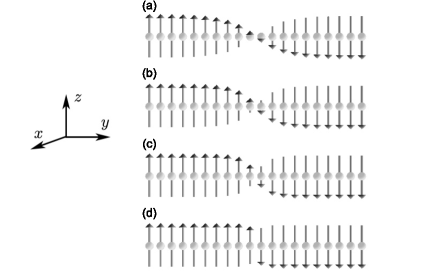
Figure 1: The magnetization $\left\langle S_{n}^{z}\right\rangle$ in the ground state of the subspace of total magnetization $M=0$, generated by the power method. The parameters are: (a) $\Delta=1.05$, (b) $\Delta=1.1$, (c) $\Delta=1.2$, (d) $\Delta=2$. The total number of spins in the spin chain is $N=20$. It is clear that there is a DW at the centre of the spin chain. Furthermore there is no structure in the XY plane, that is, $\left\langle S_{n}^{x}\right\rangle=\left\langle S_{n}^{y}\right\rangle=0$.

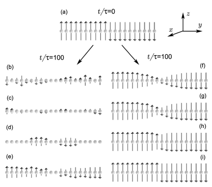
Figure 2: Top picture (a): Initial spin configuration at time $t/\tau=0$; Bottom pictures (b,c,d,e,f,g,h,i): Spin configuration at time $t/\tau=100$; Bottom left pictures (b,c,d,e): DW structures disappear or are not stable. The parameters are: (b) $\Delta=0$ (XY model), (c) $\Delta=0.5$ (Heisenberg-XY model), (d) $\Delta=1$ (Heisenberg model), (e) $\Delta=1.05$ (Heisenberg-Ising model); Bottom right pictures (f,g,h,i): DW structures are dynamically stable in the Heisenberg-Ising model. The parameters are: (f) $\Delta=1.1$, (g) $\Delta=1.2$, (h) $\Delta=2$, (i) $\Delta=20$. The total number of spins in the spin chain is $N=20$.

Now we consider $\left\langle S_{n}^{z}\right\rangle$ of the bound state $\left|\psi_{k}\right\rangle$ in the case that the number of flipped spin is half of the total spins, i.e., $k=N/2$ and $N$ is an even number. Even though the formal expression for $\left|\psi_{k}\right\rangle$ is known, the expression for $\left\langle S_{n}^{z}\right\rangle$ in this state (for finite and infinite chains) is not known. For finite $N$, the ground state in the subspace of total magnetization $M=0$ can, in principle, be calculated from Eq. (5). However, this requires a numerical procedure and we loose the attractive features of the analytical approach. Indeed, it is more efficient to use a numerical method and compute directly the ground state in the subspace of total magnetization $M=0$. In Fig. 1, we show some representative results as obtained by the power methodWilkinson99 for a chain of $N=20$ spins. In all cases, the domain wall is well-defined. Obviously, because we are considering the system in the ground state, the magnetization profile will not change during the time evolution.

To inject a DW in the spin chain, we take the state $|\Phi\rangle$ with the left half of the spins up and the other half down as the initial state (see Fig. 2(a) for $N=20$). The state $|\Phi\rangle$ corresponds to the state with the largest weight in the bound state $|\psi_{k}\rangle$ with $k=N/2$, because $|B_{m_{1}m_{2}...m_{k}}|^{2}$ reaches the maximum if $m_{i}=i$ for all $i=1,2,..,N/2$ (note $|v_{i}|<1$). It is clear that $|\Phi\rangle$ is not an eigenstate of the Hamiltonian in Eq. (1). The energy of $|\Phi\rangle$, relative to the ferromagnetic ground state, is $J\Delta/2$, and its spread $(\langle\Phi|H^{2}|\Phi\rangle-\langle\Phi|H|\Phi\rangle^{2})^{1/2}=J/2$. In Table 1, we list some representative values of the energy in the initial state (see Fig. 2(a)) and in the ground state of subspace $M=0$ (see Fig. 1).

A priori, there is no reason why the DW of the initial state $|\Phi\rangle$ should relax to a DW profile that is dynamically stable. For $\Delta\simeq 1$, the difference between energy of the initial state and the ground state energies for $N=16,18,20,22$ is relatively large and the relative spread in energy ($1/\Delta$) is large also, suggesting that near the quantum critical point, the initial state may contain a significant amount of excited states. Therefore, it is not evident that a DW structure will survive in the long-time regime. In fact, from the numbers in Table I, one cannot predict whether or not the DW will be stable. For instance, for $\Delta=1.05$ and $N=16,18,20$, the DW is not dynamically stable whereas for $N=22$ it is stable but the energies (see first line in Table I) do not give a clue as to why this should be the case. On the other hand, by solving the time dependent Schrödinger equation (TDSE), it is easy to see if the DW is dynamically stable or not.

Table 1: The energy $E=J\Delta/2$ of the initial state $|\Phi\rangle$ (see Fig. 2(a)) and the ground state $E_{g}^{(N)}$ in the $M=0$ subspace, both relative to the ground state energy of the ferromagnet.

$\Delta$	$E$	$E_{g}^{(16)}$	$E_{g}^{(18)}$	$E_{g}^{(20)}$	$E_{g}^{(22)}$
$1.05$	$0.53$	$0.16$	$0.16$	$0.16$	$0.16$
$1.1$	$0.55$	$0.23$	$0.23$	$0.23$	$0.23$
$2$	$1.00$	$0.87$	$0.87$	$0.87$	$0.87$
$5$	$2.50$	$2.45$	$2.45$	$2.45$	$2.45$

III Dynamically Stable Domain Walls

We solve the TDSE of the whole system with the Hamiltonian in Eq. (1) and study the time-evolution of the magnetization at each lattice site. The numerical solution of the TDSE is performed by the Chebyshev polynomial algorithm, which is known to yield extremely accurate independent of the time step usedTALE84 ; LEFO91 ; IITA97 ; DOBR03 . We adopt open boundary conditions, not periodic boundary conditions, because the periodic boundary condition would introduce two DWs in the initial state. In this paper, we display the results at time intervals of $\tau=\pi/5J$, and use units such that $\hbar=1$ and $J=1$.

The initial state of the system is shown in Fig. 2(a). The spins in the left part ($n=1$ to $10$) of the spin chain are all ”spin-up” and the rest ($n=11$ to $20$) are all ”spin-down”. Here ”spin-up” or ”spin-down” correspond to the eigenstates of the single spin $1/2$ operator $S_{n}^{z}$.

Whether the DW at the centre of the spin chain is stable or unstable depends on the value of $\Delta$. In Fig. 2(b,c,d,e,f,g,h, and i), we show the states of the system as obtained by letting the system evolve over a fairly long time ($t=500J/\pi$). It is clear that the DW totally disappears for $0\leq\Delta\leq 1$, that is, in the XY, Heisenberg-XY and Heisenberg spin $1/2$ chain, the DW structures are not stable. For the Heisenberg-Ising model ($\Delta>1$), the DW remains stable when $t\geq 500J/\pi$ (see Ref.Yuan06 ), and its structure is more sharp and clear if $\Delta$ is larger, so we will concentrate on the cases $\Delta>1$. One may note that the values of $\Delta$ in Fig. 2(e,f,g,h) are the same as in Fig. 1(a,b,c,d), but that the distributions of the magnetization are similar but not the same. This is because the energy is conserved during the time evolution and the system, which starts from the initial state shown in Fig. 2(a), will never relax to the ground state of the subspace with the total magnetization $M=0$.

In order to get a quantitative expression of the width of DW, we first introduce the quantity $\overline{S_{n}^{z}\left(t_{1},t_{2};\Delta\right)}$ ($n=1,2,...,N$) as the time average of the expectation value $\left\langle S_{n}^{z}\left(t\right)\right\rangle$ of $n$th spin:

$$\overline{S_{n}^{z}\left(t_{1},t_{2};\Delta\right)}\equiv\frac{\int_{t_{1}}^{t_{2}}\left\langle S_{n}^{z}\left(t\right)\right\rangle dt}{t_{2}-t_{1}}.$$ (13)

We take the average in Eq. (13) over a long period during which the DW is dynamically stable. In Fig. 3,

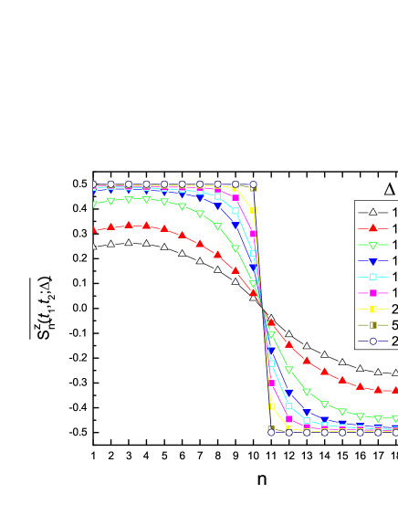
Figure 3: (Color online) $\overline{S_{n}^{z}\left(t_{1},t_{2};\Delta\right)}$ as a function of $n$ for different $\Delta$. Here $t_{1}=101\tau$, $t_{2}=200\tau$. We show the data for $\Delta=1.05,1.06,1.1,1.2,1.3,1.5,2,5$ and $20$ only. The total number of spins in the spin chain is $N=20$.

we show some results of $\overline{S_{n}^{z}\left(t_{1},t_{2};\Delta\right)}$ for the Heisenberg-Ising model, where we take $t_{1}=101\tau$, $t_{2}=200\tau$ and various $\Delta$. We find that each curve in Fig. 3 is symmetric about the line $n=\left(N+1\right)/2$, and can be fitted well by the function

$$\overline{S_{n}^{z}\left(t_{1},t_{2};\Delta\right)}=a_{\Delta}\tanh\left[\frac{n-(N+1)/2}{b_{\Delta}}\right].$$ (14)

The values of $\Delta$ we used and the corresponding values of $a_{\Delta}$, $b_{\Delta}$ are shown in Table 2. As we mentioned earlier, GochevGochev83 constructed an eigenstate of the one-dimensional anisotropic ferromagnetic spin $1/2$ chain in which the mean values $S_{n}^{z}$, $S_{n}^{x}$ and $S_{n}^{y}$ coincide with the stable DW structure in the classical spin chain, that is

$$\left\langle S_{n}^{z}\right\rangle=\frac{1}{2}\tanh(n-n_{0})\sigma,$$ (15)

where $n_{0}$ is the position of the DW (in our notation, this is $\left(N+1\right)/2$). The fitted form of $\overline{S_{n}^{z}\left(t_{1},t_{2};\Delta\right)}$ in Eq. (14) is similar to Eq. (15). From Table 2, it is clear that as $\Delta$ increases, $\left|a_{\Delta}\right|$ converges to $1/2$, in agreement with Eq. (15). From the comparison of $b_{\Delta}$ and $1/\sigma$ in Fig. 4, it is clear that the dependence on $\Delta$ is qualitatively similar but not the same. This is due to the fact that Gochev’s solution is for a DW in the ground state whereas we obtain the DW by relaxation of the state shown in Fig. 2(a).

We want to emphasize that the meaning of $\overline{S_{n}^{z}\left(t_{1},t_{2};\Delta\right)}$ in Eq. (14) is different from $\left\langle S_{n}^{z}\right\rangle$ in Eq. (15). The former describes the mean value of $\left\langle S_{n}^{z}\left(t\right)\right\rangle$ in a state with dynamical fluctuations, while the latter describes the distribution of $\left\langle S_{n}^{z}\right\rangle$ in an exact eigenstate without dynamical fluctuations.

Table 2: The values of $\Delta$ we used in our simulations and the corresponding $a_{\Delta}$, $b_{\Delta}$ fitted by Eq. (14) for a spin chain of $N=20$ spins.

$\Delta$	${a}_{\Delta}$	${b}_{\Delta}$	$\Delta$	${a}_{\Delta}$	${b}_{\Delta}$
$1.05$	$-0.263$	$3.659$	$1.8$	$-0.493$	$0.524$
$1.06$	$-0.330$	$3.171$	$1.9$	$-0.494$	$0.488$
$1.07$	$-0.377$	$2.850$	$2$	$-0.495$	$0.460$
$1.08$	$-0.406$	$2.673$	$2.1$	$-0.495$	$0.436$
$1.09$	$-0.424$	$2.534$	$2.2$	$-0.496$	$0.416$
$1.1$	$-0.435$	$2.396$	$2.5$	$-0.497$	$0.370$
$1.15$	$-0.462$	$1.996$	$3$	$-0.498$	$0.322$
$1.2$	$-0.471$	$1.626$	$4$	$-0.499$	$0.270$
$1.25$	$-0.476$	$1.330$	$5$	$-0.499$	$0.240$
$1.3$	$-0.479$	$1.142$	$6$	$-0.500$	$0.220$
$1.35$	$-0.481$	$0.959$	$7$	$-0.500$	$0.206$
$1.4$	$-0.483$	$0.869$	$8$	$-0.500$	$0.195$
$1.45$	$-0.485$	$0.770$	$9$	$-0.500$	$0.187$
$1.5$	$-0.487$	$0.719$	$10$	$-0.500$	$0.179$
$1.6$	$-0.489$	$0.629$	$15$	$-0.500$	$0.156$
$1.7$	$-0.491$	$0.568$	$20$	$-0.500$	$0.141$

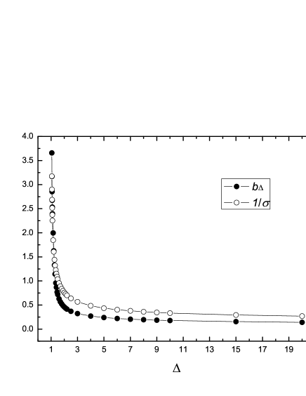
Figure 4: Comparison of $b_{\Delta}$ and $1/\sigma$ as a function of $\Delta$. The total number of spins in the spin chain is $N=20$.

Figure 5: The DW width as a function of $\Delta$ in a spin chain of $N=20$ spins. The black dots are the simulation data and the solid line is given by $W\left(\Delta\right)=A_{N}/\ln\left\{\Delta-\epsilon_{N}+\left[\left(\Delta-\epsilon_{N}\right)^{2}-1\right]^{1/2}\right\}+B_{N}$ with $\epsilon_{N}=0.046\pm 0.001,$ $A_{N}=2.16\pm 0.06$ and $B_{N}=-0.485\pm 0.068$.

Figure 6: The DW width as a function of $\Delta$ in a spin chain of $N=16$, $18$, $22$, and $24$ spins. The black dots are the simulation data and the solid line in each panel is given by Eq. (18).

Table 3: The values of $\epsilon_{N}$, $A_{N}$ and $B_{N}$ in Eq. (18) for a spin chain of $N=16$, $18$, $20$, $22$ and $24$ spins. For the fits, we used all the data for $\Delta\leq 5$.

$N$	$\epsilon_{N}$	$A_{N}$	$B_{N}$
$16$	$0.065\pm 0.001$	$2.08\pm 0.10$	$-0.493\pm 0.142$
$18$	$0.052\pm 0.002$	$2.07\pm 0.11$	$-0.450\pm 0.152$
$20$	$0.045\pm 0.002$	$2.22\pm 0.09$	$-0.556\pm 0.133$
$22$	$0.040\pm 0.001$	$2.36\pm 0.08$	$-0.689\pm 0.140$
$24$	$0.033\pm 0.001$	$2.34\pm 0.06$	$-0.681\pm 0.127$

Figure 7: Fit of $\Delta_{N}^{\ast}$ to $\Delta^{\ast}+\lambda\cdot N^{-2}$ with $\Delta^{\ast}=1.009\pm 0.002$, and $\lambda=14.253\pm 0.660$.

Figure 8: The DW width as a function of $\Delta$ ($1.06\leq\Delta\leq 20$) in the ground state of subspace $M=0$ in a spin chain of $N=20$ spins. The black dots are the simulation data and the solid line is given by Eq. (18), with $\epsilon_{N}=0.010\pm 0.001,$ $A_{N}=1.87\pm 0.04$ and $B_{N}=-0.550\pm 0.079$.

Next we introduce a definition of the DW width. From Eq. (14), we can find $n_{1}$ and $n_{2}$ which satisfy

$$\overline{S_{n_{1}}^{z}\left(t_{1},t_{2};\Delta\right)} =1/4,$$

$$\overline{S_{n_{2}}^{z}\left(t_{1},t_{2};\Delta\right)} =-1/4,$$ (16)

that is, when $\left|\overline{S_{n}^{z}\left(t_{1},t_{2};\Delta\right)}\right|$ equals half of its maximum value ($1/2$). Here $n_{1}$ and $n_{2}$ are not necessarily integer numbers. Now we can define the DW width $W$ as the distance between $n_{1}$ and $n_{2}$:

$$W=\left|n_{1}-n_{2}\right|.$$ (17)

Clearly, the width of the DW becomes ill-defined if it approaches the size of the chain. On the other hand, the computational resources (mainly memory), required to solve the TDSE, grow exponentially with the number of spins in the chain. These two factors severely limit the minimum difference between $\Delta$ and the quantum critical point ($\Delta=1$) that yields meaningful results for the width of the DW. Indeed, for fixed $N$, $\Delta$ has to be larger than the ”effective” critical value for the finite system in order for the DW width to be smaller than the system size. Although the system sizes that are amenable to numerical simulation are rather small for present-day ”classical statistical mechanics” standards, it is nevertheless possible to extract from these simulations useful information about the quantum critical behavior of the dynamically stable DW.

In Fig. 5, we plot $W$ as a function of $\Delta$ ($1.06\leq\Delta\leq 20$). By trial and error, we find that all the data can be fitted very well by the function

$$W\left(\Delta\right)=\frac{A_{N}}{\ln\left\{\Delta-\epsilon_{N}+\left[\left(\Delta-\epsilon_{N}\right)^{2}-1\right]^{1/2}\right\}}+B_{N},$$ (18)

where $\epsilon_{N}$, $A_{N}$ and $B_{N}$ are fitting parameters. As shown in Fig. 6, all the data for $N=16$, $18$, $22$, $24$ and $\Delta\leq 5$ fit very well to Eq. (18). The results of these fits are collected in Table 3.

To analyze the finite-size dependence in more detail, we adopt the standard finite-size scaling hypothesisLandau2000 . We assume that in the infinite system, the DW width plays the role of the correlation length, that is, we assume that

$$W\left(\Delta\right)\sim W_{0}(\Delta-1)^{-\nu},$$ (19)

where $\nu$ is a critical exponent. Finite-size scaling predicts that the effective critical value $\Delta_{N}^{\ast}=1+\epsilon_{N}$ where $\epsilon_{N}$ is proportional to $N^{-1/\nu}$. Taking $\nu=1/2$, Fig. 7 shows that $\Delta_{N}^{\ast}$ converges to one as $N$ increases.

As a check on the fitting procedure, we apply it to the data obtained by solving for the ground state in the $M=0$ subspace. In view of Eq. (13) and (14), we may expect that Eq. (18) fits the data very well and, as shown in Fig. 8, this is indeed the case.

If we fit the data to

$$W\left(\Delta\right)=W_{0}\left(\Delta-\Delta_{N}^{\ast}\right)^{-C}.$$ (20)

without assuming a priori value $C$, we find that $C$ depends on the range of $\Delta$ that was used in the fit, as shown in Fig. 9. Remarkably, we find that $C\approx 0.57$ if we fit the data for a large range of $\Delta$’s and that $C$ approaches $1/2$ if we restrict the value of $\Delta$ to the vicinity of the critical point.

Figure 9: The exponent $C$ as a function of $\Delta_{\max}$ in a spin chain of $N=20$ spins. The exponent $C$ obtained by fitting the DW width to Eq. (20), with $\Delta_{N=20}^{\ast}$ as obtained from the fit shown in Fig. 7, for $\Delta$ in the range $\left[1.06,\Delta_{\max}\right]$.

IV The Stability of Domain Walls

To describe the stability of the DW structure, we introduce $\delta_{n}\left(\Delta\right)$ ($n=1,2,...,N$):

$$\delta_{n}\left(\Delta\right)=\sqrt{\overline{\left[S_{n}^{z}\left(t_{1},t_{2};\Delta\right)\right]^{2}}-\overline{S_{n}^{z}\left(t_{1},t_{2};\Delta\right)}^{2}},$$ (21)

where

$$\overline{\left[S_{n}^{z}\left(t_{1},t_{2};\Delta\right)\right]^{2}}\equiv\frac{\int_{t_{1}}^{t_{2}}\left\langle S_{n}^{z}\left(t\right)\right\rangle^{2}dt}{t_{2}-t_{1}}.$$ (22)

In order to show the physical meaning of $\delta_{n}$, we write $\left\langle S_{n}^{z}\left(t\right)\right\rangle$ as

$$\left\langle S_{n}^{z}\left(t\right)\right\rangle\equiv C_{n}+\Omega_{n}\left(t\right),$$ (23)

where $C_{n}$ is a constant and $\Omega_{n}\left(t\right)$ is a time-dependent term. Then Eq. (21) becomes

$$\delta_{n}\left(\Delta\right)=\left\{\frac{\int_{t_{1}}^{t_{2}}\Omega_{n}^{2}\left(t\right)dt}{t_{2}-t_{1}}-\left[\frac{\int_{t_{1}}^{t_{2}}\Omega_{n}\left(t\right)dt}{t_{2}-t_{1}}\right]^{2}\right\}^{1/2}.$$ (24)

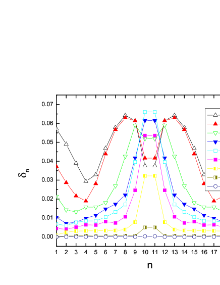
Figure 10: (Color online) $\delta_{n}\left(\Delta\right)$ as a function of $n$ for different $\Delta$. Here $t_{1}=101\tau$, $t_{2}=200\tau$. We only show the data for $\Delta=1.05,1.06,1.1,1.2,1.3,1.5,2,5$ and $20$. The total number of spins in the spin chain is $N=20$.

Figure 11: $\delta_{10}\left(\Delta\right)$ as a function of $\Delta$. Here $t_{1}=101\tau$, $t_{2}=200\tau$. The total number of spins in the spin chain is $N=20$.

It is clear that if $\left\langle S_{n}^{z}\left(t\right)\right\rangle$ is a constant in the time interval $[t_{1},t_{2}]$, then $\delta_{n}\left(\Delta\right)=0$. In general, since the initial state is not an eigenstate of the Hamiltonian Eq. (1), the magnetization of each spin will fluctuate and $\Omega_{n}\left(t\right)\neq 0$. If, after long time, the system relaxes to a stationary state that contains a DW, the magnetization of each spin will fluctuate around its stationary value $C_{n}$. The fluctuations are given by $\Omega_{n}\left(t\right)$. If $\left|\Omega_{n}\left(t\right)\right|$ is large, the difference between the actual magnetization profile at time $t$ and the stationary profile $C_{n}$ may be large. From Eq. (24), it is clear that $\delta_{n}\left(\Delta\right)$ is a measure of the deviation of $\left\langle S_{n}^{z}\left(t\right)\right\rangle$ from its stationary value $C_{n}$, averaged over the time interval $[t_{1},t_{2}]$. Thus, $\delta_{n}\left(\Delta\right)$ gives direct information about the dynamics stability of the DW.

Figure 10 shows the distribution $\delta_{n}\left(\Delta\right)$ for different values of $\Delta$. We only show some typical results, as in Fig. 3. As expected, the distribution of $\delta_{n}\left(\Delta\right)$ is symmetric about the centre of the spin chain ($n=10.5$).

We first consider how $\delta_{n}\left(\Delta\right)$ changes with $\Delta$ for fixed $n$. From Fig.10, we conclude:

1) For the spins which are not located at the DW centre, i.e., $n\neq 10,11$, $\delta_{n}\left(\Delta\right)$ decreases if $\Delta$ becomes larger. This means that the quantum fluctuations of these spins become smaller if we increase the value of $\Delta$. This is reasonable because with increasing $\Delta$, the initial state approaches an eigenstate of the Hamiltonian for which $\delta_{n}\left(\Delta\right)=0$ (Ising limit).

2) For the spins at the DW centre, i.e., $n=10,11$, when $\Delta$ becomes larger and larger, $\delta_{n}\left(\Delta\right)$ first increases and then decreases. Qualitatively, this can be understood in the following way. When $\Delta$ is close to $1$, the magnetization at the DW centre disappears very fast and remains zero. However, if $\Delta>>1$, the magnetization at the DW centre will retain its initial direction, hence the behavior of  the spin at the DW centre will qualitatively change as $\Delta$ moves away from the critical point $\Delta=1$. In Fig. 11, we plot $\delta_{10}\left(\Delta\right)$ ($=\delta_{11}\left(\Delta\right)$) as a function of $\Delta$. It is clear that $\delta_{10}\left(\Delta\right)$ first increases as $\Delta$ increases, reaches its maximum at $\Delta=1.3$, and then decreases as $\Delta$ becomes larger.

Now we consider the $n$-dependence of $\delta_{n}\left(\Delta\right)$ for fixed $\Delta$. Since $\delta_{n}\left(\Delta\right)$ is a symmetric function of $n$, we may consider only one side of the whole chain, e.g., the spins with $n=1,2,...,N/2$. From Fig.10, according to the value of $\Delta$, there are three different regions:

1) $1.05\leq\Delta\leq 1.3$: starting from the boundary ($n=1$), $\delta_{n}\left(\Delta\right)$ first decreases, then increases, and finally decreases again as $n$ approaches the DW centre ($n=10$). As we discussed already, the fluctuation of the magnetization at the DW centre is small when $\Delta$ is close to $1$. The spin at the boundary only interacts with one nearest spin, so it has more freedom to fluctuate. For the others, because of the influence of the DW structure (or boundary), the fluctuations of the spins which are near the DW (or near the boundary) are larger compared to those of a spin located in the middle of a polarized region. Thus $\delta_{n}\left(\Delta\right)$ is larger if the spin is located near the DW or near a boundary.

2) $1.3\leq\Delta\leq 5$: $\delta_{n}\left(\Delta\right)$ reaches its maximum at the DW centre. The reason for this is that in this regime the magnetizations of all spins retain their initial direction, therefore the spins that are far from the centre fluctuate little.

3) $5<\Delta$: in this regime (Ising limit), the initial state is very close to the eigenstate, and the fluctuations are small, even for the spins at the DW.

V Summary

In the presence of Ising-like anisotropy, DWs in a ferromagnetic spin $1/2$ chain are dynamically stable over extended periods of time. The profiles of the magnetization of the DW are different from the profile in the ground state in the subspace of total magnetization $M=0$. As the system becomes more isotropic, approaching the quantum critical point, the width of the DW increases as a power law, with an exponent equal to $1/2$.

References

- (1) T. Kajiwara, M. Nakano, Y. Kaneko, S. Takaishi, T. Ito, M. Yamashita, A. Igashira-Kamiyama, H. Nojiri, Y. Ono and N. Kojima, J. Am. Chem. Soc. 127 10150 (2005).
- (2) M. Mito, H. Deguchi, T. Tajiri, S. Takagi, M. Yamashita and H. Miyasaka, Phys. Rev. B 72, 144421 (2005).
- (3) H. Kageyama, K. Yoshimura, K. Kosuge, M. Azuma, M. Takano, H. Mitamura and T. Goto, J. Phys. Soc. Jpn. 66, 3996 (1997).
- (4) A. Maignana, C. Michel, A.C. Masset, C. Martin and B. Raveau, Eur. Phys. J. B 15, 657 (2000).
- (5) J. Torrance and M. Tinkham, Phys. Rev. 187, 587 (1969).
- (6) D. Nicoli and M. Tinkham, Phys. Rev. B 9, 3126 (1974).
- (7) S. Yuan, H. De Raedt, and S. Miyashita, J. Phys. Soc. Jpn., 75, 084703 (2006).
- (8) I.G. Gochev, JETP Lett. 26, 127 (1977).
- (9) I.G. Gochev, Sov. Phys. JETP 58, 115 (1983).
- (10) S. Sachdev, Quantum Phase Transitions, (Cambridge University Press, Cambridge, 1999).
- (11) H.J. Mikeska, S. Miyashita and G.H. Ristow, J. Phys.: Condens. Matter 3, 2985 (1991).
- (12) J. des Cloizeaux and M. Gaudin, J. Math. Phys. 7, 1384 (1966).
- (13) D.C. Mattis, The Theory of Magnetism I, Solid State Science Series 17 (Springer, Berlin 1981).
- (14) J.H. Wilkinson, The Algebraic Eigenvalue Problem, (Oxford University Press, Oxford, 1999).
- (15) H. Tal-Ezer and R. Kosloff, J. Chem. Phys. 81, 3967 (1984).
- (16) C. Leforestier, R.H. Bisseling, C. Cerjan, M.D. Feit, R. Friesner, A. Guldberg, A. Hammerich, G. Jolicard, W. Karrlein, H.-D. Meyer, N. Lipkin, O. Roncero and R. Kosloff, J. Comp. Phys. 94, 59 (1991).
- (17) T. Iitaka, S. Nomura, H. Hirayama, X. Zhao, Y. Aoyagi and T. Sugano, Phys. Rev. E56, 1222 (1997).
- (18) V.V. Dobrovitski and H.A. De Raedt, Phys. Rev. E67 , 056702 (2003).
- (19) D.P. Landau and K. Binder, A Guide to Monte Carlo Simulations in Statistical Physics, (Cambridge University Press, Cambridge, 2000).