Geometric phase of an atom inside an adiabatic radio frequency potential

Abstract

We investigate the geometric phase of an atom inside an adiabatic radio frequency (rf) potential created from a static magnetic field (B-field) and a time dependent rf field. The spatial motion of the atomic center of mass is shown to give rise to a geometric phase, or Berry’s phase, to the adiabatically evolving atomic hyperfine spin along the local B-field. This phase is found to depend on both the static B-field along the semi-classical trajectory of the atomic center of mass and an “effective magnetic field” of the total B-field, including the oscillating rf field. Specific calculations are provided for several recent atom interferometry experiments and proposals utilizing adiabatic rf potentials.

I Introduction

Magnetic trapping is an important enabling technology for the active research field of neutral atomic quantum gases. A variety of trap potentials can be developed using magnetic (B-) fields with different spatial distributions and time variations. For instance, the widely used quadrupole trap and the Ioffe-Pritchard trap IPT are usually created with static B-fields, while the time averaged orbiting potential (TOP) TOP and time orbiting ring trap (TORT) TORT ; Kurn1 are created using oscillating B-fields with frequencies larger than the effective trap frequencies. Atom chips atomchip have brought further developments to magnetic trap technology, as they can provide larger B-fields and gradients at reduced power-consumptions or electric currents using micro-fabricated coils. Today, magnetic trapping is a versatile tool used in many laboratories around the world for controlling atomic spatial motion in regions of different scales and geometric shapes, e.g., 3D or 2D traps, double well traps, and storage ring traps IPT ; TOP ; TORT ; Kurn1 ; atomchip ; Chapman ; ring-2 .

Recently, magnetic traps based on adiabatic microwave micro-theory ; micro-experiment and adiabatic radio frequency (rf) potentials (ARFP) Rf-collision ; Rf-previous-theory ; Rf-previous-hot ; Rf-zhanghaichao ; Rf-classical ; Rf-quantum ; Rf-experiment ; Rf-experiment2 ; Rf-experiment3 ; demarco ; Rf-cooling ; Rf-shanghai ; Rf-ring ; Rf-ring2 ; Rf-beyond ; Rf-Zimmermann ; Rf-combine have attracted considerable attention. An ARFP is typically created with the combination of a static B-field and an rf field. The idea for an ARFP has been around for some time Rf-collision ; Rf-zhanghaichao ; Rf-previous-theory , and experimental demonstrations recently have been carried out for confining both thermal Rf-previous-hot and Bose condensed atoms Rf-experiment ; Rf-experiment2 ; Rf-experiment3 ; demarco . Further development of improved ARFP with atom chip technology likely will assist in practical applications of atom interferometry. For instance, a double well potential was constructed recently using low order multi-poles capable of atomic beam splitting while maintaining tight spatial confinement Rf-classical . Several interesting recent proposals outline the construction of small storage rings with radii of the order $1\mu$m Rf-classical ; Rf-quantum ; Rf-combine ; Rf-ring ; Rf-ring2 , which could become useful if implemented for atom Sagnac interferometry Sagnac setups on atom chips.

When a neutral atom is confined in a magnetic potential, its hyperfine spin is assumed to follow adiabatically the spatial variation of the B-field direction during its spatial translational motion. As a result of this adiabatic approximation, the center of mass motion for the atom experiences an induced gauge field sun and other , giving rise to a geometric phase (or Berry’s phase) to the atomic internal spin state berry ; jorg . The effect of this geometric phase is widely known, and is first addressed carefully in a meaningful way for atomic quantum gases by an explicit calculation of the resulting geometric phase in a static or a time averaged magnetic trap in Ref. Ho-Shenoy . Several important consequences are predicted to occur for a magnetically trapped atomic condensate in a quadrupole trap, a Ioffe-Pritchard trap Ho-Shenoy ; peng-prl , or a TORT based storage ring peng-pra . To our knowledge, this geometric phase effect has not been investigated in any detail for an atom inside an ARFP.

In a recent paper, we show that this geometric phase causes an effective Aharonov-Bohm-type ABeffect phase shift in a magnetic storage ring based atom interferometer peng-pra . In addition, our studies imply that the spatial fluctuation of the geometric phase can lead to a reduction of the visibility of the interference contrast. In view of this, we decided to carry out this study as reported here for the atomic geometric phase in an ARFP in order to shed light on the proposed high precision atom Sagnac interference experiment Sagnac .

Analytical derivations for this study at some places become rather tedious and complicated. We therefore first will summarize our major results here for readers who may not be interested in the intricate details. We find that the geometric phase in an ARFP generally takes a more complicated form in comparison to the case of a static trap or a time averaged trap. In an ARFP, this phase factor is found to be determined by the trajectory of the time independent component of the trap field as well as an “effective B-field” that depends on the total B-field. In contrast to the earlier result found for a static trap or a time averaged trap Ho-Shenoy ; peng-pra , the final result turns out to be not expressible as a functional of the trajectory for the direction of the total B-field in the parameter space.

This paper is organized as follows. In sec. II, we generalize the semi-classical approach as outlined in Ref. Rf-classical for the operating principle of an ARFP to a form more convenient for discussing the geometric phase. Section III parallels that of sec. II by reformulating a full quantum theory for discussing the geometric phase inside an ARFP Rf-quantum . The explicit expression for the geometric phase inside an ARFP is given in a readily adaptable form for specifical calculations. In sec. IV, we discuss the effect of the geometric phase in several types of ARFP recently proposed for atomic splitters and storage rings Rf-classical ; Rf-quantum ; Rf-combine ; Rf-ring ; Rf-ring2 and beam splitters Rf-experiment ; Rf-classical . Finally, concluding remarks are given in sec. V.

II A semi-classical approach

In this section, we provide a semi-classical formulation for calculating the atomic geometric phase inside an ARFP. The semi-classical working principle for an ARFP is described in Ref. Rf-classical , although only for the special case when the atomic center of mass is assumed at a fixed location. In order to calculate the geometric phase, our formulation allows for the explicit consideration of atomic center of mass motion classically. In our approach, the geometric phase is obtained naturally, and the validity conditions for both the adiabatic and the rotating wave approximations are clearly shown for an ARFP.

Inside an ARFP Rf-classical , the total B-field ${\vec{B}}(\vec{r},t)$ is the sum of a static field component ${\vec{B}}_{s}(\vec{r})$ and an oscillatory rf field ${\vec{B}}_{o}(\vec{r},t)$, which conveniently is expressed as

$${\vec{B}}_{o}(\vec{r},t)={\vec{B}}^{(a)}_{\rm{rf}}(\vec{r},t)\cos(\omega t)+{\vec{B}}^{(b)}_{\rm{rf}}(\vec{r},t)\cos(\omega t+\eta).$$ (1)

where $\vec{r}$ is the spatial position vector of the atom, $\omega$ is frequency of the rf field, and $\eta$ is a relative phase factor.

In this section, we will assume that the atomic spatial motion is pre-determined, i.e., $\vec{r}(t)$ is given (as a slowly varying function of time $t$). For weak B-fields, the system Hamiltonian is simply the linear Zemman interaction

$$H(t)=g_{F}\mu_{B}{\vec{F}}\cdot{\vec{B}}[\vec{r}(t),t],$$ (2)

where $g_{F}$ is the corresponding Lande g-factor and $\mu_{B}$ denotes the Bohr magneton. $\hbar=1$ is assumed.

For a static or a time averaged magnetic trap, the Hamiltonian (2) varies slowly over time scales of the Larmor precession of the atomic spin in the total B-field. During the effectively slow trapped motion, the atomic hyperfine spin is assumed to be fixed at the instantaneous eigenstate of the Hamiltonian (2). The geometric phase then can be calculated straightforwardly from the variation of the B-field direction in the parameter space Ho-Shenoy ; peng-pra .

In an ARFP, the situation is more complicated. Although the variation of $\vec{B}_{s}[\vec{r}(t)]$ remains much slower than the Larmor precession, the rf frequency $\omega$ usually is assumed to be nearly resonant with the precession frequency. Thus, the Hamiltonian (2) contains both fast and slow time varying components, making the direct calculation of the geometric phase a more involved task. In the following, we will proceed step by step, clarifying the various approximations adopted along the way.

To understand the working principle for an ARFP, we first decompose the Hamiltonian $H(t)$ (2) into the following form

$$H(t)=H_{s}[\vec{r}(t)]+H_{+}[\vec{r}(t)]e^{-i\omega t}+H_{-}[\vec{r}(t)]e^{i\omega t},$$ (3)

where $H_{s}$ and $H_{\pm}$ are all slow varying functions of time and are given by

$$H_{s}[\vec{r}(t)] = g_{F}\mu_{B}{\vec{F}}\cdot{\vec{B}}_{s}[\vec{r}(t)],$$

$$H_{+}[\vec{r}(t)] = \frac{1}{2}g_{F}\mu_{B}{\vec{F}}\cdot\left({\vec{B}}^{(a)}_{\rm{rf}}[\vec{r}(t)]+e^{-i\eta}{\vec{B}}^{(b)}_{\rm{rf}}[\vec{r}(t)]\right),$$

$$H_{-}[\vec{r}(t)] = H_{+}^{\dagger}[\vec{r}(t)].$$ (4)

$H_{s}$ is diagonal in the spin angular momentum basis defined along the local direction of the static B-field $\vec{B}_{s}[\vec{r}(t)]$. The eigenstate takes the familiar form $|m_{F}[\vec{r}(t)]\rangle_{s}$, quantized along the direction of $\vec{B}_{s}[\vec{r}(t)]$, with the eigenvalue $m_{F}\left|B_{s}[\vec{r}(t)]\right|$ for $\vec{B}_{s}[\vec{r}(t)]\cdot\vec{F}$ and $m_{F}\in[-F,F]$, in analogy with the usual case of the z-quantized representation result of $F_{z}|m_{F}\rangle_{z}=m_{F}|m_{F}\rangle_{z}$.

Next we introduce a unitary transformation

$$U(t)=\sum_{m_{F}=-F}^{F}|m_{F}\rangle_{z}\,{}_{s}\langle m_{F}[\vec{r}(t)]|e^{im_{F}\kappa\omega t},$$ (5)

with $\kappa={\rm sign}(g_{F})$ for the rotating wave approximation. The quantum state in the interaction picture $|\Psi(t)\rangle_{I}=U(t)|\Psi(t)\rangle$ defined by $U(t)$ is governed by the Schroedinger equation $i\partial_{t}|\Psi(t)\rangle_{I}=H_{I}(t)|\Psi(t)\rangle_{I}$, with the Hamiltonian in the interaction picture given by

$$H_{I}(t) = UHU^{\dagger}+i(\partial_{t}U)U^{\dagger}$$ (6)

$$= \sum_{m=-F}^{F}m\kappa\Delta[\vec{r}(t)]|m\rangle_{z}\,{}_{z}\langle m|-i\sum_{m,n=-F}^{F}|m\rangle_{z}\,{}_{s}\langle m[\vec{r}(t)]|\frac{d}{dt}|n[\vec{r}(t)]\rangle_{s}\,{}_{z}\langle n|e^{i(m-n)\kappa\omega t}$$

$$+\sum_{m=-F+1}^{F}\left(h^{(+)}_{m}[\vec{r}(t)]|m\rangle_{z}\,{}_{z}\langle m-1|+h^{(-)}_{m}[\vec{r}(t)]|m\rangle_{z}\,{}_{z}\langle m-1|e^{2i\kappa\omega t}+h.c.\right)$$

$$+\sum_{m=-F}^{F}\left(h_{m}[\vec{r}(t)]|m\rangle_{z}\,{}_{z}\langle m|e^{i\kappa\omega t}+h.c.\right),\ \ \ \$$

where the time dependent parameters are defined as

$$\Delta[\vec{r}(t)] = \mu_{B}|g_{F}\vec{B}[\vec{r}(t)]|-\omega,$$

$$h^{(\pm)}_{m}[\vec{r}(t)] = \,{}_{s}\langle m[\vec{r}(t)]|H_{\pm}[\vec{r}(t)]|(m-1)[\vec{r}(t)]\rangle_{s},\ \ {\rm and}$$ (7)

$$h_{m}[\vec{r}(t)] = \,{}_{s}\langle m[\vec{r}(t)]|H_{\pm}[\vec{r}(t)]|m[\vec{r}(t)]\rangle_{s}.$$

The above result is obtained easily if we note that the matrix element $\,{}_{s}\langle m[\vec{r}(t)|H_{\pm}(t)|m^{\prime}[\vec{r}(t)\rangle_{s}$ is non-zero only when $m-m^{\prime}=0,\pm 1$. So far, we have always assumed that $|m[\vec{r}(t)]\rangle_{s}$ is a single valued function of the atomic position $\vec{r}$. A careful examination shows that the eigenstate $|m[\vec{r}(t)]\rangle_{s}$ cannot be determined uniquely because of the presence of the $U(1)$ gauge freedom for selecting a local phase factor $\exp\{i\phi[\vec{r}(t)]\}$, which consequently affects the resulting expressions for $h_{m}^{(\pm)}(t)$ and $\,{}_{s}\langle m[\vec{r}(t)]|d/dt|m^{\prime}[\vec{r}(t)]\rangle_{s}$.

The rotating wave approximation neglects of the oscillating terms proportional to $e^{im\omega t}$ ($m\neq 0$) in the Hamiltonian $H_{I}$ (6). The error for this approximation is estimated easily from a time dependent perturbation calculation. The sufficient condition for its validity requires that all factors such as $\int_{0}^{t}dt^{\prime}h_{m}(t^{\prime})\exp[i\kappa\omega t^{\prime}]$, $\int_{0}^{t}dt^{\prime}h_{m}^{(-)}(t^{\prime})\xi_{m,m-1}(t^{\prime})\exp[i\kappa(2\omega+\Delta)t^{\prime}]$, and $\int_{0}^{t}dt^{\prime}\langle m[\vec{r}(t^{\prime})]|d/dt^{\prime}|n[\vec{r}(t^{\prime})]\rangle\xi_{mn}(t^{\prime})\exp[i(m-n)\kappa(\omega+\Delta)t^{\prime}]$ are negligible, where

$$\xi_{mn}(t) = \exp\left[\int_{0}^{t}dt^{\prime}\,_{s}\langle m[\vec{r}(t^{\prime})]|\frac{d}{dt^{\prime}}|m[\vec{r}(t^{\prime})]\rangle_{s}\right]\times$$ (8)

$$\exp\left[-\int_{0}^{t}dt^{\prime}\,_{s}\langle n[\vec{r}(t^{\prime})]|\frac{d}{dt^{\prime}}|n[\vec{r}(t^{\prime})]\rangle_{s}\right].$$

Thus, the gauge independent factors $h_{m}^{(-)}\xi_{m,m-1}$, $\langle m_{s}|d/dt|n_{s}\rangle\xi_{mn}$ , $h_{m}$, and $\Delta$ should all vary slowly with time and with the modulus of their amplitudes much less than $\omega$.

The effective Hamiltonian in the interaction picture under the rotating wave approximation then becomes

$$H^{(I)}_{\rm eff}(t) = \mu_{B}g_{F}\vec{F}\cdot\vec{B}^{\rm eff}[\vec{r}(t)]$$ (9)

$$-i\sum_{m=-F}^{F}|m\rangle_{z}\,{}_{s}\langle m[\vec{r}(t)]|\frac{d}{dt}|m[\vec{r}(t)]\rangle_{s}\,{}_{z}\langle m|,\ \ \ \ \$$

where the first term resembles a coupling between the atomic spin and an “effective B-field” $\vec{B}^{\rm eff}(\vec{r})$, whose components in real space are given by

$$B_{x}^{\rm eff}(\vec{r}) = {\rm Re}\left[\frac{2\,_{s}\langle m(\vec{r})|H_{\pm}(\vec{r})|(m-1)(\vec{r})\rangle_{s}}{\mu_{B}g_{F}\sqrt{(F+m)(F-m-1)}}\right],$$

$$B_{y}^{\rm eff}(\vec{r}) = -{\rm Im}\left[\frac{2\,_{s}\langle m(\vec{r})|H_{\pm}(\vec{r})|(m-1)(\vec{r})\rangle_{s}}{\mu_{B}g_{F}\sqrt{(F+m)(F-m-1)}}\right],\ \ {\rm and}$$

$$B_{z}^{\rm eff}(\vec{r}) = \left|\vec{B}_{s}(\vec{r})\right|-\frac{\omega}{\mu_{B}|g_{F}|}\ .\ \ \$$ (10)

Clearly, the $x$- and $y$-components of the effective field $\vec{B}^{\rm eff}(\vec{r})$ depend on the explicit form of the eigenstate $|m(\vec{r})\rangle_{s}$. In fact, it easily can be seen that different choices of the local phase factor for the $|m(\vec{r})\rangle_{s}$ actually lead to different values of $\vec{B}^{\rm eff}(\vec{r})$ related to each other through $\vec{r}$-dependent rotations in the $x$-$y$ plane.

In practice, the eigenstate $|n(\vec{r})\rangle_{s}$ and the effective field $\vec{B}^{\,\rm eff}$ can sometimes be constructed more simply, as in Ref. Rf-classical . For any spatial position $\vec{r}$, we first choose a rotation $R[\hat{m}(\vec{r}),\chi(\vec{r})]$ along the axis $\hat{m}(\vec{r})$ with an angle $\chi(\vec{r})$ that satisfies $R[\vec{n}(\vec{r}),\chi(\vec{r})]\vec{B}_{s}(\vec{r})=|\vec{B}_{s}(\vec{r})|\hat{e}_{z}$. It is then easy to show that the eigenstate $|n[\vec{r}(t)]\rangle_{s}$ can be chosen as

$$|n(\vec{r})\rangle_{s}=\exp\left[i\vec{F}\cdot\hat{m}(\vec{r})\chi(\vec{r})\right]|n\rangle_{z}.$$ (11)

Unfortunately, the choice for $R$ is not unique in a given static field $\vec{B}_{s}(\vec{r})$, an analogous result to the $U(1)$ gauge freedom for the the egienstate $|n(\vec{r})\rangle_{s}$. Corresponding to the choice (11) given above for $|n(\vec{r})\rangle_{s}$, the unitary transformation $U$ defined in (5) would become

$$U(t)=\exp(-iF_{z}\omega t)\cdot\exp\left[-i\vec{F}\cdot\hat{m}(\vec{r})\chi(\vec{r})\right],$$ (12)

and the transverse components of the “effective B-field” given by $B^{\,\rm eff}_{x,y}(\vec{r})=\overline{B}_{x,y}(\vec{r})/2$ Rf-classical with

$$\overline{\vec{B}}(\vec{r}) = R[\hat{m}(\vec{r}),\chi(\vec{r})]\vec{B}_{\rm rf}^{(a)}(\vec{r})$$ (13)

$$+R[\hat{e}_{z},-\kappa\eta]R[\hat{m}(\vec{r}),\chi(\vec{r})]\vec{B}_{\rm rf}^{(b)}(\vec{r}).$$

In earlier discussions of an ARFP Rf-classical ; Rf-quantum , the atomic internal state is assumed uniformly to remain adiabatically in a certain eigenstate of the first term of $H^{(I)}_{\rm eff}(t)$. To fully appreciate this adiabatic approximation and to calculate the geometric phase, we expand $|\Psi(t)\rangle_{I}$ into the instantaneous eigenstate basis $|n[\vec{r}(t)]\rangle_{\rm eff}$ quantized along the direction of the effective B-field $\vec{B}^{\rm eff}$ according to $|\Psi(t)\rangle_{I}=\sum_{n}C_{n}(t)|n[\vec{r}(t)]\rangle_{\rm eff}$. The first term of $H^{(I)}_{\rm eff}(t)$ is simply the effective Zemman interaction between the atomic hyperfine spin and the effective B-field. The corresponding Schroedinger equation for the Hamiltonian $H^{(I)}_{\rm eff}(t)$ of (9) then becomes

$$i\frac{d}{dt}C_{n}(t)=[\epsilon_{I}^{(n)}(t)+\nu_{nn}(t)]C_{n}(t)+\sum_{m\neq n}\nu_{nm}(t)C_{m}(t),$$

with

$$\epsilon_{I}^{(n)}(t) = n\mu_{B}g_{F}|\vec{B}^{\rm eff}(t)|,$$

$$\nu_{pq}(t) = -i\sum_{l}\,{}_{\rm eff}\langle p[\vec{r}(t)]|l\rangle_{z}$$ (14)

$$\,{}_{s}\langle l[\vec{r}(t)]|\frac{d}{dt}|l[\vec{r}(t)]\rangle_{s}\,{}_{z}\langle l|q[\vec{r}(t)]\rangle_{\rm eff}$$

$$-i\,_{\rm eff}\langle p[\vec{r}(t)]|\frac{d}{dt}|q[\vec{r}(t)]\rangle_{\rm eff}.$$

Under the adiabatic approximation, the atomic internal state remains in a given eigenstate $|n[\vec{r}(t)]\rangle_{\rm eff}$ with transitions to states $|m[\vec{r}(t)]\rangle_{\rm eff}$ ($m\neq n$) being negligibly small. Thus, the transition probability, as estimated from the first order perturbation theory,

$$\int_{0}^{t}dt^{\prime}\nu_{nm}(t^{\prime})e^{i\int_{0}^{t^{\prime}}dt^{\prime\prime}[\epsilon_{I}^{(n)}(t^{\prime\prime})+\nu_{nn}(t^{\prime\prime})-\epsilon_{I}^{m}(t^{\prime\prime})-\nu_{mm}(t^{\prime\prime})]}$$

should be much less than one. As before, we find the sufficient condition for the validity of the adiabatic approximation is given by

$$\frac{|\nu_{mn}(t)|}{|\epsilon_{I}^{m}(t^{\prime})-\epsilon_{I}^{(n)}(t^{\prime})|}\ll 1,$$ (15)

provided that $\nu_{mn}(t)\exp[i\int_{0}^{t^{\prime}}[\nu_{nn}(t^{\prime\prime})-\nu_{mm}(t^{\prime\prime})]dt^{\prime}]$, which is independent of the local phase factor for $|n[\vec{r}(t)]\rangle_{\rm eff}$ and $|n[\vec{r}(t)]\rangle_{s}$, remains a slowly varying function of time.

A straight forward calculation from the effective Hamiltonian (9) then gives the general expression for the geometric phase in an ARFP

$$\gamma_{n}(t) = \int_{0}^{t}\nu_{nn}(t^{\prime})dt^{\prime}$$ (16)

$$= -i\int_{0}^{t}\sum_{l}\left|\,{}_{\rm eff}\langle n[\vec{r}(t^{\prime})|l\rangle_{z}\right|^{2}\times$$

$$\,{}_{s}\langle l[\vec{r}(t^{\prime})]|\frac{d}{dt^{\prime}}|l[\vec{r}(t^{\prime})]\rangle_{s}dt^{\prime}$$

$$+\gamma^{(I)}_{n}(t),$$

and $\gamma^{(I)}_{n}(t)=-i\int_{0}^{t}dt^{\prime}\,_{\rm eff}\langle n[\vec{r}(t^{\prime})|d/dt^{\prime}|n[\vec{r}(t^{\prime})\rangle_{\rm eff}$. During the adiabatic motion in a given internal state, the time evolution of the coefficient $C_{n}(t)$ takes the form

$$C_{n}(t)=C_{n}(0)e^{-i\int_{0}^{t}\epsilon_{I}^{(n)}(t^{\prime})dt^{\prime}}e^{-i\gamma_{n}(t)}.$$ (17)

Equation (16) is the central result of this work. The geometric phase of an atom inside an ARFP is shown to contain two parts. The second part, $\gamma^{(I)}_{n}(t)$, is clearly due to the interaction term $\mu_{B}g_{F}\vec{F}\cdot\vec{B}^{{\rm eff}}$ in $H_{\rm eff}^{(I)}$ (9), with its value determined by the trajectory of the direction for the “effective B-field” $\vec{B}^{\rm eff}$. The first part arises from the second term of $H_{\rm eff}^{(I)}$ (9). It is determined by the trajectories of both the static field $\vec{B}_{s}$ and the effective B-field $\vec{B}^{\rm eff}$. The expression for $\gamma_{n}$ in an ARFP is complicated because the internal quantum state in an ARFP is assumed to be adiabatically kept in an eigenstate of $\mu_{B}g_{F}\vec{F}\cdot\vec{B}^{\rm eff}$, rather than an eigenstate of the total interaction Hamiltonian $H^{(I)}_{\rm eff}(t)$.

In section IV, we will perform explicit calculations for several examples of ARFP proposed for various applications: e.g., as atomic storage rings or atomic beam splitters. Most often we find that only the first part of Eq. (16) contributes a non-zero value to the geometric phase.

Before proceeding to the next section for a quantal treatment of the geometric phase, we find the time evolution of the atomic spin state in the Schroedinger picture

$$|\Psi(t)\rangle = \sum_{ml}C_{l}(0)\,_{z}\langle m|l[\vec{r}(t)]\rangle_{\rm eff}\times$$ (18)

$$e^{-i\int_{0}^{t}\epsilon_{I}^{l}(t^{\prime})dt^{\prime}}e^{-i\gamma_{l}(t)}e^{-im\omega t}|m[\vec{r}(t)]\rangle_{s},$$

obtained directly from $|\Psi(t)\rangle=U^{\dagger}(t)|\Psi(t)\rangle_{I}$ after the applications of the rotating wave and adiabatic approximations. When the atom is prepared initially in a specific adiabatic state $|n[\vec{r}(t)]\rangle_{\rm eff}$ of the interaction picture, we arrive at the simple case of $C_{l}(0)=\delta_{ln}$.

III A quantum mechanical treatment

In the previous section, we provided the result for the geometric phase $\gamma_{n}(t)$ in an ARFP based on a semi-classical approach, where the atomic center of mass motion is described classically. A clear physical picture exists in this case for the appearance of the geometric phase in a certain parameter space. The validity conditions for the rotating wave and the adiabatic approximations as obtained above are all formulated in terms of gauge independent forms. However, if the influence of the geometric phase on the atomic spatial motion is to be included, e.g., as in the Aharonov-Bohm-type, phase shift, interference arrangement in an atomic Sagnac interferometer discussed earlier peng-pra , we would need an improved description where both the atomic spin and its center of mass motion are treated quantum mechanically.

In a full quantum treatment of the atomic motion, the quantum state of an atom can be expressed as $|\Phi(t)\rangle=\sum\phi_{l}(\vec{r},t)|l\rangle_{z}$, where $\phi_{l}(\vec{r},t)$ is the atomic spatial wave function for the internal state $|l\rangle_{z}$ of $F_{z}$. The state $|\Phi(t)\rangle$ then satisfies the Schroedinger equation governed by the Hamiltonian

$${\cal H}=\frac{{\vec{P}}^{2}}{2M}+g_{F}\mu_{B}\vec{F}\cdot\vec{B}(\vec{r},t),$$ (19)

with $\vec{P}$ being the kinetic momentum and $M$ the atomic mass.

The rotating wave and adiabatic approximations can be introduced now by defining the interaction picture with the unitary transformation

$${\cal U}(t) = \left[\sum_{m=-F}^{F}|m\rangle_{z}\,{}_{\rm eff}\langle m(\vec{r})|\right]\times$$ (20)

$$\left[\sum_{n=-F}^{F}|n\rangle_{z}\,{}_{s}\langle n(\vec{r})|e^{in\kappa\omega t}\right].\ \ \$$

The state in the interaction picture $|\Phi(t)\rangle_{I}={\cal U}(t)|\Phi(t)\rangle$ now is governed by the Schroedinger equation with the Hamiltonian ${\cal H}_{\rm eff}={\cal U}{\cal H}{\cal U}^{\dagger}$. Under the rotating wave and adiabatic approximations, we neglect transitions between states $|m\rangle_{z}$ and $|n\rangle_{z}$ $(m\neq n)$ as well as the rapidly oscillating terms. We then obtain

$${\cal H}_{\rm eff} \approx \sum_{n}|n\rangle_{z}\,{}_{z}\langle n|{\cal H}_{\rm eff}|n\rangle_{z}\,{}_{z}\langle n|$$ (21)

$$\approx \sum_{n}H_{\rm ad}^{(n)}|n\rangle_{z}\,{}_{z}\langle n|,$$

where the adiabatic Hamiltonian $H_{\rm ad}^{(n)}$ for the $n$-th adiabatic branch is defined as

$$H_{\rm ad}^{(n)}=\frac{\left(\vec{P}-\vec{A}_{n}\right)^{2}}{2M}+\epsilon_{I}^{(n)}(\vec{r}),$$ (22)

with the effective gauge potential

$$\vec{A}_{n}(\vec{r}) = -i\sum_{l}\left|\,{}_{\rm eff}\langle n(\vec{r})|l\rangle_{z}\right|^{2}\,_{s}\langle l(\vec{r})|\nabla|l(\vec{r})\rangle_{s}$$ (23)

$$-i\,_{\rm eff}\langle n(\vec{r})|\nabla|n(\vec{r})\rangle_{\rm eff}.$$

In this form, it is well known that the geometric phase $\gamma_{n}$ can be expressed as the integral of the gauge potential $\vec{A}_{n}$ along the spatial trajectory for the atomic center of mass in an ARFP, i.e., one would expect generally that $\gamma_{n}=\int\vec{A}_{n}\cdot d\vec{r}$. Similar to the result of the semi-classical approach, the gauge potential $\vec{A}_{n}(\vec{r})$ can be expressed as the sum of two parts. The first part in Eq. (23) is the weighted sum of the atomic gauge potential $-i\,_{s}\langle l(\vec{r})|\nabla|l(\vec{r})\rangle_{s}$ from the static field $\vec{B}_{s}$, while the second term is the atomic gauge potential from the “effective B-field” $\vec{B}^{\rm eff}$.

A full quantum treatment for atomic motion in an ARFP has been attempted earlier Rf-quantum . In fact, many of our formulations are identical to the results of Ref. Rf-quantum . For instance, it is easy to show that the unitary transformations $U_{S}$, $U_{R}$, and $U_{F}$ in Rf-quantum are related directly to ours as $U_{F}^{\dagger}U_{R}^{\dagger}U_{S}^{\dagger}={\cal U}$. The only difference concerns the gauge potential $\vec{A}_{n}$ that was neglected in Ref. Rf-quantum . Thus, they did not give the expression for the gauge potential, and the result for the geometric phase was not obtained either Rf-quantum . Our study shows that the neglect of the adiabatic gauge potential potentially can give rise to a final result, dependent on the choice of the local phase factors for the internal eigenstate.

IV Geometric phases in ARFP based applications

In the above two sections, we obtain the expression for the atomic geometric phase in an ARFP. This section is devoted to the calculations of the geometric phases for several proposed applications of ARFP, such as storage rings or beam splitters for neutral atoms Rf-ring ; Rf-ring2 ; Rf-combine ; Rf-classical ; Rf-quantum .

Before presenting our results for the more specific cases, we provide some general discussions of the geometric phases in several ARFP based storage rings. As was pointed out earlier, the geometric phase $\gamma_{n}$ is given by the line integral of the gauge potential $\vec{A}_{n}$ along the trajectory for the atomic center of mass motion. For a closed path in the storage ring at a fixed $\rho=\rho_{c}$ and $z=z_{c}$, this can be further reduced to

$$\gamma_{n}=q\int_{0}^{2\pi}A^{(\phi)}_{n}(\rho,\phi,z)\rho d\phi,$$ (24)

where the integer $q$ is the winding number of the path and $A^{(\phi)}_{n}$ is the component of $\vec{A}_{n}$ along the azimuthal direction $\hat{e}_{\phi}$ of the familiar cylindrical coordinate system $(\rho,\phi,z)$. Without loss of generality, we take $q=1$ in this paper. For the storage rings proposed in Refs. Rf-ring ; Rf-ring2 ; Rf-combine ; Rf-classical ; Rf-quantum , the gauge potentials $A^{(\phi)}_{n}(\rho,\phi,z)$ are actually independent of the angle $\phi$. Therefore, the geometric phase is simply given by

$$\gamma_{n}^{(c)}=2\pi\rho_{c}A^{(\phi)}_{n}(\rho_{c},z_{c}),$$ (25)

given out in explicit forms for different storage ring schemes Rf-classical ; Rf-quantum ; Rf-combine ; Rf-ring ; Rf-ring2 .

In reality, because of thermal motion or when the atomic transverse motional state is considered, the center of mass for an atom can deviate from $(\rho_{c},z_{c})$ even for a closed trajectory. This uncertainty in the exact shape of the closed trajectory gives rise to a fluctuating geometric phase and is usually difficult to study. Assuming a simple closed path at fixed $\rho$ and $z$, we have found previously that the subsequently fluctuations could decrease the visibility of the interference pattern peng-pra . Quantum mechanically, such destructive interference can be explained as resulting from entanglement between the freedoms for $\phi$ and $(\rho,z)$ because of the dependence of the gauge potential $A_{n}^{\phi}$ on $\rho$ and $z$. Therefore, it is important to investigate this dependence near the trap center.

For simplicity, our discussions below will focus on the closed loops where $\rho$ and $z$ are $\phi$-independent constants. In this case, the geometric phase can be expressed as $\gamma_{n}(\rho,z)=2\pi\rho A^{(\phi)}_{n}(\rho,z)$. We will show numerically the distributions for $\gamma_{n}(\rho,z)$ obtained this way near the central region of $(\rho_{c},z_{c})$. If needed, a more rigorous approach can be developed to investigate the fluctuations of the resulting geometric phase from the gauge potential $A^{(\phi)}_{n}(\rho,z)$.

IV.1 The storage ring proposals of Refs. Rf-ring ; Rf-ring2 ; Rf-combine

This subsection is devoted to a detailed calculation of the geometric phases for the ARFP storage ring proposals of Refs. Rf-ring ; Rf-ring2 ; Rf-combine . We will derive the analytical expressions for the azimuthal component $A^{(\phi)}_{n}$ of the gauge potential that arises in both cases from cylindrically symmetric static B-field and rf fields. Because of the cylindrical symmetry, the angle $\beta_{s}(\rho,z)$ between the local static B-field and the $z$-axis is required to be analytical in the region near the storage ring. Therefore, the eigenstate $|n(\vec{r})\rangle_{s}$ of $\vec{F}\cdot\vec{B}_{s}$ can be chosen as

$$|n(\vec{r})\rangle_{s}=\exp\{-i[\vec{F}\cdot\hat{e}_{\phi}\beta_{s}(\rho,z)+n\phi]\}|n\rangle_{z}.$$ (26)

Consequently, $\vec{B}^{\,\rm eff}(\vec{r})$ is also cylindrically symmetric, which leads to the eigenstate $|n(\vec{r})\rangle_{\rm eff}$ of $\vec{F}\cdot\vec{B}^{\,\rm eff}$ as

$$|n(\vec{r})\rangle_{\rm eff}=\exp\{-i[\vec{F}\cdot\hat{n}^{\,\rm eff}_{\perp}(\vec{r})\beta_{\rm eff}(\rho,z)+n\phi]\}|n\rangle_{z},$$ (27)

with the unit vector $\hat{n}^{\,\rm eff}_{\perp}(\vec{r})$ in the $x$-$y$ plane orthogonal to $\vec{B}^{\,\rm eff}(\vec{r})$ and $\beta_{\,\rm eff}(\rho,z)$ denoting the angle between $\vec{B}^{\,\rm eff}(\vec{r})$ and the $z$-axis. We note that the unit vector field $\hat{n}^{\,\rm eff}_{\perp}(\vec{r})$ also possesses cylindrical symmetry, i.e., remains invariant under rotation around the $z$-axis. The expressions of (26) and (27) allow us to obtain the simple expression of the gauge potential

$$A^{(\phi)}_{n}(\rho,z)=-\frac{n}{\rho}\cos\beta_{\rm eff}(\rho,z)\cos\beta_{s}(\rho,z),$$ (28)

after straightforward calculations.

In the scheme of Ref. Rf-ring , the static B-field is a “ring-shaped quadrupole field” that vanishes along a circle of a radius $\rho_{0}$ in the $x$-$y$ plane. Near $\rho=\rho_{0}$, the B-field is given approximately by

$$\vec{B}_{s}(\vec{r})=B^{\prime}(\rho-\rho_{0})\hat{e}_{\rho}-B^{\prime}z\hat{e}_{z},$$ (29)

like a quadrupole field, while the rf-field takes a complicated form

$$\vec{B}_{o}(\vec{r},t) = \left(\frac{a}{\sqrt{2}}\cos(\omega t)+\frac{b}{\sqrt{2}}\cos(\omega t+\varphi)\right)\hat{e}_{\rho}$$ (30)

$$+\left(-\frac{a}{\sqrt{2}}\sin(\omega t)+\frac{b}{\sqrt{2}}\sin(\omega t+\varphi)\right)\hat{e}_{z},\ \ \ \ \ \$$

with constants $a$ and $b$ independent of $\vec{r}$.

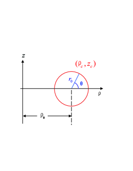
Figure 1: (Color online) A cross-sectional view for the storage ring of Ref. Rf-ring . The static field is zero in the ring at the fixed radius $\rho_{0}$. The addition of rf-fields creates an ARFP centered at a ring through $(\rho_{c},z_{c})$. The distance from the trap center to the ring with radius $\rho_{0}$ in the plane $z=0$ is $r_{0}$.

From the expression of (26) for the eigenstate $|n(\vec{r})\rangle_{s}$, the “effective B-field” $\vec{B}^{\,\rm eff}$ becomes

$$\vec{B}^{\,\rm eff}(\vec{r}) = B^{\prime}[\sqrt{(\rho-\rho_{0})^{2}+z^{2}}-r_{0}]\hat{e}_{z}$$ (31)

$$-\left(\frac{b}{\sqrt{2}}\cos(\theta+\varphi)+\frac{a}{\sqrt{2}}\cos\theta\right)\hat{e}_{\rho}$$

$$+\left(\frac{b}{\sqrt{2}}\sin(\theta+\varphi)-\frac{a}{\sqrt{2}}\sin\theta\right)\hat{e}_{\phi},$$

where $r_{0}$ and $\theta$ are given by

$$r_{0} = \frac{\omega}{|\mu_{B}g_{F}B^{\prime}|}\,,$$

$$\cos\theta(\rho,z) = \frac{\rho-\rho_{0}}{\sqrt{(\rho-\rho_{0})^{2}+z^{2}}}\,,$$

$$\sin\theta(\rho,z) = \frac{z}{\sqrt{(\rho-\rho_{0})^{2}+z^{2}}}\,.$$ (32)

In an ARFP, as discussed here, the trap center at $(\rho_{c},z_{c})$ is determined by minimizing both the $z$-component and the transverse component of $\vec{B}^{\,\rm eff}$. Without loss of generality, we will assume $a,b>0$. Then, $(\rho_{c},z_{c})$ is found to satisfy

$$\theta(\rho_{c},z_{c}) = -\varphi/2,$$

$$\sqrt{(\rho_{c}-\rho_{0})^{2}+z_{c}^{2}} = r_{0},$$ (33)

i.e., the trap center lies on the surface of the “resonance toroid” at $\rho=\rho_{0}$ with a radius $r_{0}$ as shown in Fig. 1. The relative angle of the trap center with respect to the center of the toroid cross-section is given by $-\varphi/2$. On this “resonance toroid,” the rf-field is resonant with the static field, i.e., $B^{\,\rm eff}_{z}$ vanishes. As a result, the “effective B-field” lies again in the $x$-$y$ plane on the “resonance toroid,” which gives $\cos\beta_{\rm eff}(\rho_{c},z_{c})=0$ and leads to the result $A^{(\phi)}_{n}(\rho_{c},z_{c})=\gamma_{n}=0$ as shown in the trap center for the storage ring considered before in Ref. Rf-ring .

From the expression (29) of the static field and the definition of the angle $\theta(\rho,z)$, we find a simple relationship $\beta_{s}(\rho,z)=\pi/2+\theta(\rho,z)$, with which the gauge potential $A^{(\phi)}_{n}(\rho,\phi)$ in (28) can be further simplified as

$$A^{(\phi)}_{n}(\rho,z) = \frac{n}{\rho}\cos\beta_{\rm eff}(\rho,z)\sin\theta(\rho,z)$$ (34)

$$\approx \frac{n}{\rho}\cos\beta_{\rm eff}(\rho,z)\sin\theta(\rho_{c},z_{c}),$$

near the trap center. Thus, the spatial fluctuation of the gauge potential $A^{(\phi)}_{n}(\rho,z)$ in the region around the trap center is closely related to the angle $\theta(\rho_{c},z_{c})$ of the trap center, or the parameter $\varphi$ of the oscillating field $\vec{B}_{o}$. When $\varphi=0$, the atom is trapped in the region with $\theta\approx 0$ or $\pi$, where the fluctuation of $A^{(\phi)}_{n}(\rho,z)$ is suppressed significantly due to the small value of $\sin\theta$. On the other hand, if the angle $\varphi$ is set to $\pi$ with the trap center located in the region with $\theta\approx\pm\pi/2$, the fluctuation of the gauge potential becomes amplified.

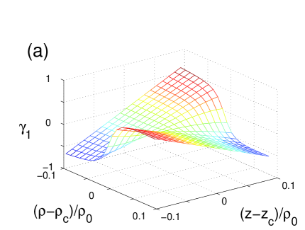
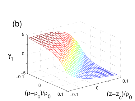
Figure 2: (Color online) The distribution of the geometric phase $\gamma_{1}$ near the trap center $(\rho_{c},z_{c})$ of the storage ring proposed in Ref. Rf-ring at (a) $\varphi=0$, (b) $\varphi=\pi/2$, and (c) $\varphi=\pi$, clearly displaying the $\sin(\varphi/2)$ dependence.

In Fig. 2, we illustrate numerical results for the distribution of the geometric phase $\gamma_{1}(\rho,z)=2\pi\rho A_{1}^{\phi}(\rho,z)$ in the region near the trap center at $\varphi=0,\pi/2,\pi$. We see clearly decreased fluctuations of $\gamma_{1}$ when the absolute value of $\sin\theta(\rho_{c},z_{c})=-\sin(\varphi/2)$ is decreased.

Next we turn to the storage ring of Ref. Rf-ring2 constructed from a quadrupole static B-field $\vec{B}_{s}(\vec{r})=B^{\prime}(x,y,-2z)$ and an $\vec{r}$-independent rf field $\vec{B}_{o}=B_{\rm rf}\cos(\omega t)\hat{e}_{z}$ along the $z$ direction. The resulting ARFP provides a 2D ring shaped trap in the $x$-$y$ plane. In addition, a 1D optical potential along the $z$ direction is employed to confine atoms in the transverse plane at $z=0$ Rf-ring2 . The “effective B-field” takes the form

$$\vec{B}^{\,\rm eff}(\vec{r})=B^{\prime}(\rho-\rho_{0})\hat{e}_{z}-\frac{1}{2}B_{\rm rf}\hat{e}_{\rho},$$ (35)

in the plane at $z=0$, with $\rho_{0}=\omega/|\mu_{B}g_{F}B^{\prime}|$. Because the strength of $\vec{B}^{\,\rm eff}$ is near minimum at the ring $\rho=\rho_{0}$, the trap center for this storage ring is located at $\rho_{c}=\rho_{0}$ and $z_{c}=0$. At the trap center, the “effective B-field” is along the direction of $\hat{e}_{\rho}$. Thus, according to Eq. (28), the geometric phase $\gamma_{n}^{(c)}$ at the trap center again vanishes.

In Fig. 3, we show the distribution of the geometric phase $\gamma_{1}$ in the region near the trap center for $B_{\rm rf}=0.05|B^{\prime}|\rho_{0}$ and $B_{\rm rf}=0.15|B^{\prime}|\rho_{0}$. We see that the fluctuation is relatively small when the strength of the rf-field is large. This can be explained by Eq. (28), which shows that $A_{n}^{(\phi)}$ is proportional to $\cos\beta_{\rm eff}$ and can be approximated as $2B^{\,\rm eff}_{z}/B_{\rm rf}$ near the trap center. When $B_{\rm rf}$ is large, the gauge potential becomes a relatively slow varying function of $\rho$ and $z$. In this case, the presence of a 1D optical potential allows for the possibility of tuning the trap center position to a nonzero value of $z$, with the storage ring remaining in the $x$-$y$ plane. Then $\cos\beta_{s}$ is assumed to a nonzero value, leading to increased fluctuations for the geometric phase.

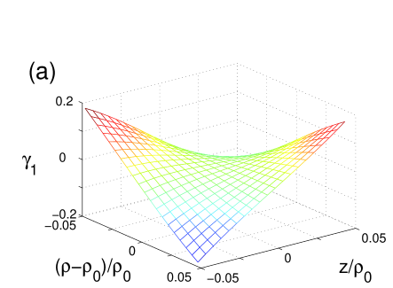
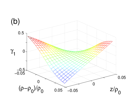
Figure 3: (Color online) The geometric phase $\gamma_{1}$ for the storage ring of Ref. Rf-ring2 with (a) $B_{\rm rf}=$ $0.15B^{\prime}\rho_{0}$ and (b) $B_{\rm rf}=0.05B^{\prime}\rho_{0}$.

Finally, we discuss the geometric phase in the “time averaged” ARFP storage ring proposed in Ref. Rf-combine . Unlike previously considered ARFP based storage rings, the time dependence now exists in both the “static B-field” and the frequency of the rf field given by

$$\vec{B}_{s}(\vec{r},t) = B^{\prime}\rho\hat{e}_{\rho}-2B^{\prime}z\hat{e}_{z}+B_{m}\sin(\omega_{m}t)\hat{e}_{z},$$

$$\vec{B}_{o}(t) = B_{\rm rf}\sin[\omega(t)t]\hat{e}_{z},$$

$$\omega(t) = \omega_{0}\sqrt{1+(B_{m}/B^{\prime}\rho_{0})^{2}\sin^{2}(\omega_{m}t)}\,.$$ (36)

The frequency $\omega_{m}$ is assumed to be much smaller than $\omega_{0}$ but much larger than the trap frequency. The radius $\rho_{0}$ is now defined as $\rho_{0}=\omega_{0}/|\mu_{B}g_{F}B^{\prime}|$, and the “effective B-field” takes the form

$$\vec{B}^{\,\rm eff}(\vec{r},t)=\Delta(\vec{r},t)\hat{e}_{z}-\frac{B^{\prime}\rho}{|2\vec{B}_{s}(\vec{r},t)|}B_{\rm rf}\hat{e}_{\phi}\,.$$ (37)

The operating principle for the time averaged storage ring of Ref. Rf-combine is similar to the well-known TOP TOP and TORT traps TORT ; Kurn1 . The effective trap potential experienced by the atom is proportional to the time averaged value of the “effective B-field” $\int_{0}^{2\pi/\omega_{m}}|\vec{B}^{\,\rm eff}(\vec{r},t)|dt$. When $B_{\rm rf}$ and $B_{m}$ are much smaller than $B^{\prime}\rho_{0}$, the center of the storage ring is located approximately at $\rho_{c}=\rho_{0},z_{c}=0$. Using the earlier result peng-pra , we find that in the time averaged storage ring, the effective gauge potential $\tilde{A}_{n}^{(\phi)}(\rho,z)$ is reduced simply to the time averaged instantaneous gauge potential

$$\tilde{A}_{n}^{(\phi)}(\rho,z)=\frac{\omega_{m}}{2\pi}\int_{0}^{2\pi/\omega_{m}}A_{n}^{(\phi)}(\rho,z,t)dt,$$ (38)

with $A_{n}^{(\phi)}(\rho,z,t)$ given in (28). The geometric phase then is given approximately by $\gamma_{n}(\rho,z)=2\pi\tilde{A}_{n}^{(\phi)}(\rho,z)$. In this case, we find that the geometric phase always vanishes at the trap center $(\rho_{c},z_{c})$. Figure 4 illustrates the distribution of the geometric phase in the region near the trap center for two different values of the rf-field amplitude $B_{\rm rf}$. Similar to the storage ring of Ref. Rf-ring2 , the fluctuation of the geometric phase is suppressed in this case for large $B_{\rm rf}$.

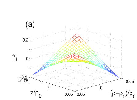
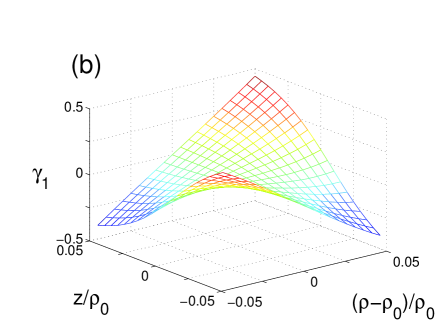
Figure 4: (Color online) The geometric phase $\gamma_{1}$ for the storage ring of Ref. Rf-combine at (a) $B_{\rm rf}=0.3B^{\prime}\rho_{0}$ and (b) $B_{\rm rf}=0.1B^{\prime}\rho_{0}$. $B_{m}=0.05B^{\prime}\rho_{0}$.

IV.2 The storage ring proposals of Refs. Rf-classical ; Rf-quantum

Next we consider the ARFP based storage ring proposed in Refs. Rf-classical ; Rf-quantum . In this case, the static B-field is that of a Ioffe-Pritchard trap on an atom chip. In the Cartesian coordinate $(x,y,z)$, it takes the form

$$\vec{B}_{s}=B^{\prime}x\hat{e}_{x}-B^{\prime}y\hat{e}_{y}+B^{\prime}L\hat{e}_{z},$$ (39)

where $B^{\prime}$ is the B-field gradient and the bias field along the $z$-direction is denoted as $B^{\prime}L$. The amplitudes $\vec{B}^{(a)}_{\rm rf}$ and $\vec{B}^{(b)}_{\rm rf}(z)$ of the rf field are $\vec{B}^{(a)}_{\rm rf}=[B_{\rm rf}(z)/\sqrt{2}]\hat{e}_{x}$ and $\vec{B}^{(b)}_{\rm rf}=[B_{\rm rf}(z)/\sqrt{2}]\hat{e}_{y}$ with

$$B_{\rm rf}(z)=B_{\rm rf}^{(0)}+B^{\prime\prime}z^{2}.$$ (40)

In the schemes of Ref. Rf-classical ; Rf-quantum considered earlier, the phase $\eta$ of the rf field is assumed to be $\kappa\pi/2$. The $x$- and $y$-components of the “effective B-field” $\vec{B}^{\,\rm eff}(\vec{r})$ then become

$$B^{\,\rm eff}_{x}(\vec{r}) = \frac{B_{\rm rf}(z)}{2\sqrt{2}}(1+\cos\beta_{s}(\rho,z)),$$

$$B^{\,\rm eff}_{y}(\vec{r}) = 0,$$ (41)

according to Eq. (10). Then the strength of the “effective B-field” $\vec{B}^{\,\rm eff}$ has its minimum along a circle with a non-zero radius $\rho_{c}$, provided a positive detuning $\Delta$ exists at the origin $(0,0,0)$ Rf-classical ; Rf-quantum . The “effective B-field” $\vec{B}^{\,\rm eff}$ is easily shown to lie in the $x$-$z$ plane along the trap bottom mapped out by the atomic center of mass motion. This gives rise to a vanishing $\gamma_{F}^{(I)}$. With a proper choice for the local phase of $|n(\vec{r})\rangle_{\rm eff}$, the gauge potential $A^{(\phi)}_{n}$ takes the form

$$A^{(\phi)}_{n}(\rho,z)=\frac{n}{\rho}\cos\beta_{\rm eff}(\rho,z)\left(1-\cos\beta_{s}(\rho,z)\right).$$ (42)

Figure 5 displays the geometric phase along a closed path for a spin-$1$ atom as a function of $\rho_{c}$ for the ARFP storage ring proposed in Refs. Rf-classical ; Rf-quantum . The parameter $\lambda$ is defined as

$$\lambda=\sqrt{2}\frac{\Delta[\vec{r}=0]}{|g_{F}\mu_{B}B_{\rm rf}^{(0)}|}\ .$$ (43)

To assure the validity of the rotating wave approximation, we find that the maximal values of $\Delta[\vec{r}=0]/(|g_{F}|\mu_{B})$ and $B_{\rm rf}^{(0)}/\sqrt{2}$ must be restricted to the region of $\lambda\in[0,0.15]$.

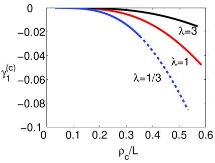
Figure 5: (Color online) The geometric phase $\gamma_{1}$ is plotted against the radius $\rho_{c}$ for the ARFP storage ring of Ref. Rf-classical ; Rf-quantum with $\eta=\kappa\pi/2$ at $\lambda=3$, $\lambda=1$, and $\lambda=1/3$. To assure the validity of the rotating wave approximation, in the solid lines, the maximal value of $\Delta[\vec{r}=0]/|g_{F}\mu_{B}B^{\prime}\rho_{0}|$ or $B_{\rm rf}/(\sqrt{2}B^{\prime}\rho_{0})$ are restricted to be smaller than $0.15$. The extending dashed line is beyond the rotating wave approximation for $\lambda=1/3$ and $B_{\rm rf}/(\sqrt{2}B^{\prime}\rho_{0})\in[0.15,0.3]$.

As shown in Fig. 1, the geometric phase remains much smaller than $2\pi$ in this situation. This fact can be appreciated easily if we look at the distribution of the “effective B-field” ${\vec{B}}^{\,\rm eff}$. According to Eq. (41), the component $B_{x}^{\,\rm eff}$ has a nonzero minimal value $B_{\rm rf}/(2\sqrt{2})$, while $|B^{\rm eff}_{z}|$ can become arbitrarily small, although not necessarily zero in general. Therefore, at the trap center where $|{\vec{B}}^{\,\rm eff}|$ is a minimum, the value of $\cos\beta_{\rm eff}=B^{\,\rm eff}_{z}/|{\vec{B}}^{\,\rm eff}|$ can become very small, leading to small geometric phases. Yet, despite the relatively small geometric phase found here, our result remains important because it could represent a systematic error if not properly included in a Sagnac interference experiment.

In Fig. 6, we show the spatial distribution of the geometric phase $\gamma_{1}$ around the trap center with $\lambda=1/3$ and $\lambda=3$. The fluctuation is found to be relatively small when $\lambda$ is small or when the rf-field amplitude $B_{\rm rf}$ is large.

Although not discussed in Refs. Rf-classical ; Rf-quantum , a ring shaped trap also can be realized if we take $\eta=-\kappa\pi/2$. The “effective B-field” $\vec{B}^{\,\rm eff}$ still lies in the $x$-$y$ plane

$$\vec{B}^{\,\rm eff}_{x}(\vec{r}) = -\frac{B_{\rm rf}(z)}{2\sqrt{2}}\cos(2\phi)(1-\cos\beta_{s}(\rho,z)),$$

$$\vec{B}^{\,\rm eff}_{y}(\vec{r}) = \frac{B_{\rm rf}(z)}{2\sqrt{2}}\sin(2\phi)(1-\cos\beta_{s}(\rho,z)),$$ (44)

clearly giving rise to a non-zero solid angle with respect to a closed path along the storage ring. Therefore, the term $\gamma^{(\rm eff)}_{F}$ is non-zero in this case. We choose the eigenstates $|n(\vec{r})\rangle_{s}$ and $|n(\vec{r})\rangle_{\rm eff}$ as

$$|n(\vec{r})\rangle_{s} = \exp[-i\vec{F}\cdot\hat{n}_{s}(\vec{r})\beta_{s}(\rho,z)]|n\rangle_{z},$$

$$|n(\vec{r})\rangle_{\rm eff} = \exp[-i\vec{F}\cdot\hat{n}^{\,\rm eff}_{\perp}(\vec{r})\beta_{\rm eff}(\rho,z)]|n\rangle_{z}.$$ (45)

with the unit vector $\hat{n}^{s}_{\perp}(\vec{r})$ in the $x$-$y$ plane orthogonal to $\vec{B}_{s}(\vec{r})$. In this case, the gauge potential $A^{(\phi)}_{n}$ can be expressed as

$$A^{(\phi)}_{n}(\rho,z)=\frac{n}{\rho}\cos\beta_{\rm eff}(\rho,z)[1+\cos\beta_{s}(\rho,z)].$$ (46)

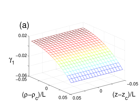
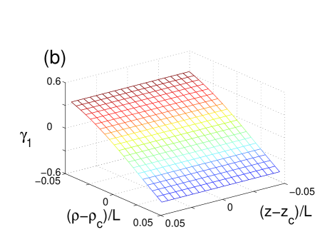
Figure 6: (Color online) The spatial distribution of the geometric phase $\gamma_{1}$ for the storage ring of Refs. Rf-classical ; Rf-quantum at (a) $\lambda=1/3$ and (b) $\lambda=3$. $\eta=\kappa\pi/2$. $B_{\rm rf}^{(0)}=0.08B^{\prime}L$ and $B^{\prime\prime}=10^{-12}B^{\prime}/L$ are assumed.

In Figure 7, we show the fluctuation of the geometric phase $\gamma_{1}$ for a closed path with a new parameter

$$\lambda^{\prime}=6\sqrt{2}\frac{\Delta[\vec{r}=0]}{|g_{F}\mu_{B}B_{\rm rf}^{(0)}|}\,,$$ (47)

equal to $3$ and $1/3$. The fluctuation for $\gamma_{1}$ is found to be much larger than the case of $\eta=\kappa\pi/2$, which can be explained by the transverse components $B^{\,\rm eff}_{x,y}$ of the “effective B-field.” Because $\cos\beta_{s}$ is always close to unity. In the case of $\eta=-\kappa\pi/2$, $B^{\,\rm eff}_{x,y}$ can take only small positive values. Therefore, at the minimum of the ARFP trap $\rho=\rho_{0}$ of $|\vec{B}^{\,\rm eff}|$, both $B^{\,\rm eff}_{z}$ and $B^{\,\rm eff}_{x,y}$ have to be close to zero. In this case the value for $\cos\beta_{\rm eff}$ becomes a rapidly changing function of $\rho$ in the region near $\rho_{c}$.

Our above calculations have obtained analytical expressions of the geometric phases in an ARFP based storage ring for $\eta=\pm\kappa\pi/2$. We have further investigated the fluctuations of the geometric phase for the two cases of $\eta=\pm\kappa\pi/2$. It seems one benefits from implementing a Sagnac interferometer in the discussed ARFP storage ring with $\eta=\kappa\pi/2$ and operating at a relatively large $\lambda$.

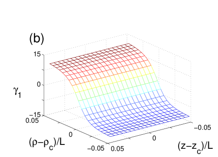
Figure 7: (Color online) The spatial distribution of the geometric phase $\gamma_{1}$ for the storage ring of Refs. Rf-classical ; Rf-quantum at (a) $\lambda^{\prime}=3$ and (b)$\lambda^{\prime}=1/3$. $\eta=-\kappa\pi/2$. $B_{\rm rf}^{(0)}=0.08B^{\prime}L$ and $B^{\prime\prime}=10^{-12}B^{\prime}/L$ are assumed.

Before proceeding onto the concluding section, we will discuss the geometric phase in an ARFP based beam splitter created via a double potential Rf-classical ; Rf-experiment . In such an implementation, the static field $\vec{B}_{s}$ is created from a Ioffe-Pritchard trap, while the oscillating rf field components are $\vec{B}_{\rm rf}^{(a)}=B_{\rm rf}[z]\hat{e}_{x}$ and $\vec{B}_{\rm rf}^{(b)}=0$. By spatially tuning the amplitude of $B_{\rm rf}$ from zero to a significant value, in the $x$-$y$ plane, an ARFP can be tuned from a single well centered near the origin to a double well with two minimal points at the point with nonzero radius $\rho_{0}$ and $\phi=0,\pi$. Therefore, a Y-shaped atom beam splitter can be accomplished when the $B_{\rm rf}[z]$ initially is increased along the $z$-axis to a large value, and then decreased to zero. In such an arrangement, the atom beam moving along the $z$ direction can be separated into two beams that move along the $z$-axis at $\phi=0,\pi$ for a while, and then can be recombined again into a single beam.

In the atom interferometer considered above, both the static field $\vec{B}_{s}$ and the “effective B-field” $\vec{B}^{\,\rm eff}$ are limited to the $x$-$z$ plane. Therefore, for motion along the closed path of the trap bottom, the solid angle enclosed by the trajectory of $\vec{B}^{\,\rm eff}$ is zero. Thus, the geometric phase in (16) can be expressed as

$$\gamma_{n}(t)=-i\int_{0}^{t}\sum_{l}|\,_{\rm eff}\langle n(\vec{r})|l\rangle_{z}|^{2}\,_{s}\langle l(\vec{r})|\nabla|l(\vec{r})\rangle_{s}\cdot\vec{v}dt^{\prime}.\ \ \$$ (48)

We can show that the product $\,{}_{\rm eff}\langle n(\vec{r})|l\rangle_{z}|^{2}\,_{s}\langle l(\vec{r})|\nabla|l(\vec{r})\rangle_{s}$ is a function of $\rho_{c}$ and is independent of $z$. Thus, the geometric phase can be expressed as an integral of this function with respect to $\rho_{c}$, from zero to a large value and then back to zero. Therefore, the value of the geometric phase would be zero in the end.

V Conclusion

In this study, we develop theoretical formalisms for the calculation of the atomic geometric phase inside an ARFP. We show that, due to the complexity of the ARFP, the geometric phase depends on the spatial variation of both the static field and an “effective B-field” $\vec{B}^{\,\rm eff}$. We provide general expressions for the geometric phase and the corresponding adiabatic gauge potential in Eqs. (16) and (23), respectively.

To shed light on actual applications of the atomic geometric phase, we investigate the distribution of atomic geometric phases for several proposed or ongoing experiments with ARFP based storage rings and atom beam splitters. We prove rigorously that the geometric phase in the center of the storage rings proposed in Refs. Rf-ring ; Rf-ring2 is always zero. In addition, we find that in the storage ring of Ref. Rf-ring , the spatial fluctuation of the geometric phase sensitively depends on the position of the trap center on the “resonance toroid.” In the proposals of Refs. Rf-ring2 ; Rf-combine ; Rf-classical ; Rf-quantum , the fluctuation for the geometric phase becomes significantly suppressed when the amplitude $B_{\rm rf}$ of the rf-field is large. In the proposals of Rf-classical ; Rf-quantum , the fluctuations of the geometric phase also is suppressed if the angle $\eta$ is set to be $\kappa 2\pi$. In the beam splitter realized with the double well potential ARFP Rf-classical ; Rf-experiment , the geometric phase is shown to be zero.

Our work helps to clarify the working principle of trapping neutral atoms in an ARFP and the validity conditions for the various approximations involved. We hope our results will shine new light on the proposed inertial sensing experiments based on trapped atoms in ARFP.

- (1) D. E. Pritchard, Phys. Rev. Lett. 51, 1336 (1983).
- (2) W. Petrich, M. H. Anderson, J. R. Ensher, and E. A. Cornell, Phys. Rev. Lett. 74, 3352 (1995).
- (3) A.S. Arnold and E. Riis, J. Mod. Opt. 49, 959 (2002); C. S. Garvie, E. Riis, and A. S. Arnold, Laser Spectroscopy XVI, edited by P. Hannaford et al. (World Scientific, Singapore, 2004), p. 178, see also www.photonics.phys.strath.ac.uk.
- (4) S. Gupta, K. W. Murch, K. L. Moore, T. P. Purdy, and D. M. Stamper-Kurn, Phys. Rev. Lett. 95, 143201 (2005); K. W. Murch, K. L. Moore, S. Gupta, and D.M. Stamper-Kurn, Phys. Rev. Lett. 96, 013202 (2005).
- (5) R. Folman, P. Krger, J. Schmiedmayer, J. Denschlag, and C. Henkel, Advances in Atomic, Molecular, and Optical Physics, vol. 48, 263 (2002).
- (6) J. A. Sauer, M. D. Barrett, and M. S. Chapman, Phys. Rev. Lett. 87, 270401 (2001).
- (7) A.S. Arnold, C.S. Garvie, and E. Riis, Phys. Rev. A 73, 041606(R) (2006).
- (8) C. C. Agosta, I. F. Silvera, H. T. C. Stoof, and B. J. Verhaar, Phys. Rev. Lett. 62, 2361 (1989).
- (9) Z. Zhao, I. F. Silvera, and M. Reynolds, Jour. Low. Temp. Phys. 89, 703 (1992).
- (10) A. J. Moerdijk, B. J. Verhaar, and T. M. Nagtegaal, Phys. Rev. A 53, 4343 (1996).
- (11) H. Zhang, P. Zhang, X. Xu, J. Han, and Y. Wang, Chin. Phys. Lett. 22, 83 (2001).
- (12) O. Zobay and B. M. Garraway, Phys. Rev. Lett. 86, 1195 (2001); Phys. Rev. A 69, 023605 (2004).
- (13) Y. Colombe, E. Knyazchyan, O. Morizot, B. Mercier, V. Lorent, and H. Perrin, Europhys. Lett. 67, 593 (2004).
- (14) S. Hofferberth, I. Lesanovsky, B. Fischer, J. Verdu, and J. Schmiedmayer, Nature Physics 2, 710 (2006).
- (15) T. Schumm, S. Hofferberth, L. M. Andersson, S. Wildermuth, S. Groth, I. Bar-Joseph, J. Schmiedmayer, and P. Krger, Nature Physics 1, 57 (2005).
- (16) G.-B. Jo, Y. Shin, S. Will, T. A. Pasquini, M. Saba, W. Ketterle, D. E. Pritchard, M. Vengalattore, and M. Prentiss, Phys. Rev. Lett. 98, 030407 (2007).
- (17) M. White, H. Gao, M. Pasienski, and B. DeMarco, Phys. Rev. A 74, 023616 (2006).
- (18) T. Fernholz, C. R. Gerritsma, P. Krger, and R. J. C. Spreeuw, arXiv:Physics/0512017.
- (19) O. Morizot, Y. Colombe, V. Lorent, and H. Perrin, arXiv: Physics/0512015.
- (20) I. Lesanovsky and W. von Klitzing, arXiv: cond-mat/0612213.
- (21) I. Lesanovsky, T. Schumm, S. Hofferberth, L. M. Andersson, P. Krger, and J. Schmiedmayer, Phys. Rev. A 73, 033619 (2006).
- (22) I. Lesanovsky, S. Hofferberth, J. Schmiedmayer, and P. Schmelcher, Phys. Rev. A 74, 033619 (2006).
- (23) C. L. G. Alzar, H. Perrin, H. B. M. Garraway, and V. Lorent, arXiv: physics/0608088.
- (24) X. Li, H. Zhang, M. Ke, B. Yan, and Y. Wang, arXiv: physics/0607034.
- (25) S. Hofferberth, B. Fishcher, T. Schumm, J. Schmiedmayer, and I. Lesanovsky, arXiv: quan-ph/0611240.
- (26) Ph.W. Courteille, B. Deh, J. Fortgh, A. Gnther, S. Kraft, C. Marzok, S. Slama, and C. Zimmermann, J. Phys. B 39, 1055 (2006).
- (27) M. G. Sagnac, C. R. Hebd. Seances Acad. Sci. 157, 708 (1913).
- (28) C. A. Mead and D. G. Truhlar, J. Chem. Phys. 70, 2284 (1979); C. A. Mead, Phys. Rev. Lett. 59, 161 (1987); C. P. Sun and M. L. Ge, Phys. Rev. D 41, 1349 (1990).
- (29) M. V. Berry, Proc. R. Soc. Lond. A 392, 45 (1984).
- (30) J. Schmiedmayer, M. S. Chapman, C. R. Ekstrom, T. D. Hammond, D. K. Kokorowski, A. Lenef, R. A. Rubenstein, E. T. Smith, and D. E. Pritchard, p. 72, Atom interferometry, edited by P. Berman, (Academic Press, N.Y. 1997).
- (31) T. Ho and V. B. Shenoy, Phys. Rev. Lett. 77, 2595 (1996).
- (32) P. Zhang, H. H. Jen, C. P. Sun, and L. You, Phys. Rev. Lett. 98, 030403 (2007).
- (33) P. Zhang and L. You, Phys. Rev. A 74, 062110 (2006).
- (34) Y. Aharonov and D. Bohm, Phys. Rev. 115, 485 (1959).