Generating Squeezed States of Nanomechanical Resonator

Abstract

We propose a scheme for generating squeezed states in solid state circuits consisting of a nanomechanical resonator (NMR), a superconducting Cooper-pair box (CPB) and a superconducting transmission line resonator (STLR). The nonlinear interaction between the NMR and the STLR can be implemented by setting the external biased flux of the CPB at certain values. The interaction Hamiltonian between the NMR and the STLR is derived by performing Fr$\rm\ddot{o}$hlich transformation on the total Hamiltonian of the combined system. Just by adiabatically keeping the CPB at the ground state, we get the standard parametric down-conversion Hamiltonian. The CPB plays the role of “nonlinear media”, and the squeezed states of the NMR can be easily generated in a manner similar to the three-wave mixing in quantum optics. This is the three-wave mixing in a solid-state circuit.

I introduction

Mechanical harmonic oscillator plays an important role in the historical development of quantum mechanics. The harmonic oscillator problem was one of the few completely solvable problems when one began to learn quantum mechanics. Due to the macroscopic nature, the experiments of mechanical harmonic oscillators didn’t achieve much progress for a quite long time, however. Recently, with the development in quantum information processing, people are now searching for possible applications of mechanical harmonic oscillator in this field, and evidence for quantized displacement in a nanomechanical harmonic oscillator has been observed Gaidarzhy . Many good physical ideas about the harmonic oscillator came up, though this system is rather simple. Squeezed state was one of them. Squeezed state provides a good example of the interplay between experiment and theory in the development of quantum mechanics. Statistical properties of squeezed states have been widely investigated and the possibility of applying squeezed states to study the fundamental quantum physics phenomena, as well as to detect the gravitational radiation, has been recognized scully ; bocko .

Though the idea of squeezed states originated from mechanical harmonic oscillator, the first experiment realization was the squeezed states of electromagnetic field in nonlinear quantum opticsslusher ; wu . In the nonlinear optical experiments, three-wave and four-wave mixing were two main methods to generate squeezed states. If one injects low energy photons into a nonlinear optical medium, the second harmonic generation may be induced and this forms a squeezed state, this procedure is called three-wave mixing. Though the theory of four-wave mixing was more complicated, the first squeezed state of electromagnetic field was implemented in this system. And recently, the theory of generating squeezed states in a high-Q cavity was considered Almeida .

Recently, there has been significant progress in realizing quantum optics in solid state electrical circuits. This new subject has a nickname “circuit quantum electrodynamics (circuit QED)” blais ; Chiorescu ; geller1 ; huo07 . The extreme strong coupling limit in cavity QED has been implemented experimentally with circuit QED systems, such as superconducting charge qubit and superconducting transmission line resonator (STLR) system wallraff , flux qubit and quantum $LC$ oscillator system Chiorescu , and phase qubit and nanomechanical resonator (NMR) system ( which is a mechanical harmonic oscillator) geller2 .

Because of the extreme strong coupling in circuit QED, generating squeezed states in such systems became very interesting and attracted much attention moon ; zhou ; rabl ; tian ; Ruskov ; xue . In Ref. moon , using two modes of the STLR coupled to a superconducting charge qubit simultaneously, the authors studied microwave parametric down-conversion and discussed the squeezed states of one mode of the STLR. In the other Refs.zhou ; rabl ; tian ; Ruskov , the authors discussed the generation of squeezed states of NMR. The generation of squeezed states of NMR in these schemes use either the operations on the qubit or dissipation and measurement to produce the needed nonlinearity.

In this paper, we propose a scheme for generating squeezed states of NMR in circuit QED, and it is similar to the three-wave mixing in optical cavity experiments. Our proposal is based on the system consisting of a superconducting Cooper-pair box (CPB), also a superconducting charge qubit, a NMR and a STLR. We find that with certain biased conditions of the CPB, the nonlinear process can be implemented and the squeezed states of NMR can easily be generated. The nonlinear interaction can be switched on and off at will by changing the external biased flux of the CPB. By controlling the gate charge $n_{g}>1/2$ and/or $n_{g}<0$, one can get different squeezed variables $x$ and/or $p$. Compared with other schemes, our scheme is more simple and effective in generating the squeezed states. In this scheme, the state of CPB is adiabatically kept in its ground states, and does not need qubit operations so that it avoids the restriction set by the decoherence time of the qubit.

II The Model

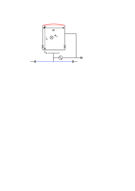
Figure 1: (Color online) Schematic diagram of combined system of a STLR, a NMR and a superconducting CPB. The STLR (the blue line) is shown at the bottom, and at the top is the NMR (the red line), which is one part of the SQUID.

The system under consideration is shown in Fig.1. A STLR (the blue line at the bottom of Fig.1) is placed close to a CPB. The state of CPB is separately controlled by the gate voltage $V_{g}$ through a gate capacitance $C_{g}$. The CPB is also coupled to a large superconductor reservoir through two identical Josephson junctions with capacitance $C_{J}$ and Josephson energy $E_{J}$, and this forms a superconducting quantum interference device (SQUID) and is also the basic configuration of superconducting charge qubit. The SQUID configuration allows one to apply external flux to control the Josephson energy. For superconducting charge qubits, the capacitance $C_{g}$ is much less than $C_{J}$. In this regime a convenient basis is formed by the charge states, characterized by the number of Cooper pairs $n$ on the CPB. In the neighborhood of $n_{g}=1/2$, only two charge states $|N\rangle$ and $|N+1\rangle$ play a role, while all other charge states, having a much higher energy, can be ignored. In this case, the Hamiltonian of the CPB reads makhlin

$$H_{q}=-\frac{1}{2}E_{c}(1-2n_{g})\sigma_{z}-E_{J}\cos(\frac{\pi\Phi_{e}}{\Phi_{0}})\sigma_{x},$$ (1)

where $E_{c}=(2e)^{2}/(2C_{\Sigma})$ is the charging energy, $C_{\Sigma}=2C_{J}+C_{g}$ is the total capacitance saw by the CPB, $n_{g}=C_{g}V_{g}/(2e)$ is the gate charge induced by the gate voltage, and $\Phi_{e}$ is the externally applied flux.

For a CPB fabricated inside a STLR, there is not only the dc voltage $V_{g}$ but also a quantum part $V_{q}$ applied on the gate capacitance. The quantized voltage at the antinode $z=L/(2k)$ of the STLR takes it’s maximum amplitude blais

$$V_{q}=\sum_{k}V_{0}^{k}(a_{k}+a_{k}^{\dagger}), V_{0}^{k}=\sqrt{\frac{\hbar\omega_{k}}{Lc}}.$$

Here, $\omega_{k}=k\pi/(L\sqrt{lc})$, with $L$, $l$ and $c$ being the length, the inductance and capacitance per unit length of the STLR, respectively. At low temperatures, there is only one mode of the STLR, say $\omega_{k}=\omega_{a}$, that couples to the CPB, then the quantum voltage applied on the gate capacitance beomes $V_{q}=V_{0}(a+a^{\dagger})$. The Hamiltonian of the joint system (STLR and CPB) has a spin-boson form

$$H_{1} = -\frac{1}{2}E_{c}(1-2n_{g})\sigma_{z}-E_{J}\cos(\frac{\pi\Phi_{e}}{\Phi_{0}})\sigma_{x}$$ (2)

$$+\frac{eC_{g}V_{0}}{C_{\Sigma}}(a+a^{\dagger})\sigma_{z}+\hbar\omega_{a}a^{\dagger}a.$$

Now we consider the coupling between the NMR and the CPB. A NMR is fabricated as a part of the SQUID, which has a length $\mathbbm{L}$ and width $\mathbbm{W}$, as shown in Fig.1. Considering the small displacement of the NMR, the effective area of the SQUID is $S=\mathbbm{W}(\mathbbm{L}+x)$, where $x$ is the displacement operator and $x=\sqrt{\hbar/(2M\omega_{b})}(b+b^{\dagger})$, with $\omega_{b}$ and $M$ being the frequency and mass of the NMR, respectively. Thus the flux bias of the SQUID is $\Phi_{e}=\Phi_{e}^{0}+B\mathbbm{W}x$, where $\Phi_{e}^{0}$ is the flux bias corresponding to the equilibrium position of the NMR zhou . With the total flux bias, the effective Josephson coupling energy of the SQUID becomes

$$E_{J}(x)=-E_{J}\cos\frac{\pi(\Phi_{e}^{0}+B\mathbbm{W}x)}{\Phi_{0}}.$$ (3)

The Hamiltonian of the total system, including STLR, NMR and CPB reads

$$H_{2} = -\frac{1}{2}E_{c}(1-2n_{g})\sigma_{z}-E_{J}\cos\frac{\pi(\Phi_{e}^{0}+B\mathbbm{W}x)}{\Phi_{0}}\sigma_{x}$$ (4)

$$+\frac{eC_{g}V_{0}}{C_{\Sigma}}(a+a^{\dagger})\sigma_{z}+\hbar\omega_{a}a^{\dagger}a+\hbar\omega_{b}b^{\dagger}b.$$

It’s obviously that the Josephson coupling energy Eq.(3) is a nonlinear function of $x$ and can be expanded to

$$E_{J}(x) = -E_{J}[\cos(\frac{\pi\Phi_{e}^{0}}{\Phi_{0}})\cos(\frac{\pi B\mathbbm{W}x}{\Phi_{0}})$$ (5)

$$-\sin(\frac{\pi\Phi_{e}^{0}}{\Phi_{0}})\sin(\frac{\pi B\mathbbm{W}x}{\Phi_{0}})].$$

In general, $x$ is very small, then the first and second term of Eq.(5) can be discarded and expanded to the first order of $x$, respectively. In this way, one can get the linearized function of Josephson coupling energy of $x$, and there is only linear interaction terms remained in Hamiltonian (4). As pointed by Zhou et al. zhou , the nonlinearity of the Josephson coupling energy in $x$ shouldn’t be neglected all the time, and it would be important for the generation of squeezed states.

III Squeezing of NMR

In the past years, two cavities interacting with a two-level atom has been widely studied benivegna ; xie ; sun , they focused on the linear interaction in such systems. Here, we study the nonlinear interaction in the STLR, NMR and CPB system. An important nonlinear effect is the generation of squeezed states, which is an outstanding task in quantum mechanics. In the following we show how we realize the nonlinear interaction and how we can use the nonlinear interaction to generate squeezed states. Our method is similar to the three-wave mixing in quantum optics.

In order to realize nonlinear interaction, one can bias the SQUID at $\Phi_{e}^{0}=m\Phi_{0}$, here $m$ is an integer, and expand the Josephson energy to the second order in $x$, then the Hamiltonian (4) becomes

$$H_{t} = \hbar\omega_{a}a^{\dagger}a+\hbar\omega_{b}b^{\dagger}b-\frac{1}{2}E_{c}(1-2n_{g})\sigma_{z}-(-1)^{m}E_{J}\sigma_{x}$$ (6)

$$+\hbar\lambda_{a}(a^{\dagger}+a)\sigma_{z}+\hbar\lambda_{b}(b^{\dagger}+b)^{2}\sigma_{x},$$

where

$$\lambda_{a}=\frac{eC_{g}}{\hbar C_{\Sigma}}\sqrt{\frac{\hbar\omega_{a}}{Lc}}, \lambda_{b}=\frac{(-1)^{m}E_{J}(\pi B\mathbbm{W})^{2}}{4M\omega_{b}\Phi_{0}^{2}}.$$

In the following we choose the eigenenergy basis (spanned by $|0\rangle=\sin(\theta/2)|N+1\rangle+\cos(\theta/2)|N\rangle$ and $|1\rangle=\cos(\theta/2)|N+1\rangle-\sin(\theta/2)|N\rangle$) to simplify the above Hamiltonian. Here, $\theta=\tan^{-1}[(-1)^{m}2E_{J}/(E_{c}(1-2n_{g}))]$ is the mixing angle. In the representation of eigenenergy basis of the CPB and under the rotating-wave approximation, the Hamiltonian (6) is simplified to

$$H = \hbar\omega_{a}a^{\dagger}a+\hbar\omega_{b}b^{\dagger}b-\frac{1}{2}\hbar\Omega\rho_{z}$$ (7)

$$+\hbar g_{a}(a^{\dagger}\rho_{-}+a\rho_{+})+\hbar g_{b}(b^{\dagger 2}\rho_{-}+b^{2}\rho_{+}),$$

where $\Omega=\sqrt{E_{c}^{2}(1-2n_{g})^{2}+4E_{J}^{2}}/\hbar$, $\rho_{z}=|0\rangle\langle 0|-|1\rangle\langle 1|$, $\rho_{+}={\rho_{-}}^{\dagger}=|1\rangle\langle 0|$, $g_{a}=-\lambda_{a}\sin\theta$ and $g_{b}=\lambda_{b}\cos\theta$.

Assuming the detunings between the CPB and the STLR and the NMR satisfy the large detuning limits, that is $|\Delta_{a}|=|\Omega-\omega_{a}|,\hskip 4.0pt|\Delta_{b}|=|\Omega-2\omega_{b}|\gg g_{a},\hskip 4.0ptg_{b}$, then the variables of the CPB can be adiabatically eliminated by performing the Fr$\rm\ddot{o}$hlich transformation frohlich on the total Hamiltonian (7). Dividing the Hamiltonian (7) into two parts $H=H_{0}+H_{I}$, with

$$H_{0}=\hbar\omega_{a}a^{\dagger}a+\hbar\omega_{b}b^{\dagger}b-\frac{1}{2}\hbar\Omega\rho_{z},$$

and

$$H_{I}=\hbar g_{a}(a^{\dagger}\rho_{-}+a\rho_{+})+\hbar g_{b}(b^{\dagger 2}\rho_{-}+b^{2}\rho_{+}).$$

Apply a unitary transformation $H_{S}=e^{-S}He^{S}$ with the generator $S=g_{a}(a^{\dagger}\rho_{-}-a\rho_{+})/\Delta_{a}+g_{b}(b^{\dagger 2}\rho_{-}-b^{2}\rho_{+})/\Delta_{b}$, and expand $H_{S}$ to second order in $g_{i}/\Delta_{i}$ ($i=a,b$), we obtain the effective Hamiltonian

$$H_{S} = \hbar(\omega_{a}-\frac{g_{a}^{2}}{\Delta_{a}}\rho_{z})a^{\dagger}a-\frac{1}{2}\hbar(\Omega+\frac{2g_{b}^{2}}{\Delta_{b}}+\frac{g_{a}^{2}}{\Delta_{a}})\rho_{z}$$ (8)

$$+\hbar(\omega_{b}+\frac{2g_{b}^{2}}{\Delta_{b}}-\frac{g_{b}^{2}}{\Delta_{b}}\rho_{z}-\frac{g_{b}^{2}}{\Delta_{b}}b^{\dagger}b\rho_{z})b^{\dagger}b$$

$$-\frac{1}{2}\hbar g_{a}g_{b}(\frac{1}{\Delta_{a}}+\frac{1}{\Delta_{b}})(a^{\dagger}b^{2}+b^{\dagger 2}a)\rho_{z}.$$

If the CPB is adiabatically kept on the ground state, the effective Hamiltonian becomes

$$H_{S} = \hbar(\omega_{a}-\frac{g_{a}^{2}}{\Delta_{a}})a^{\dagger}a+\hbar(\omega_{b}+\frac{g_{b}^{2}}{\Delta_{b}}-\frac{g_{b}^{2}}{\Delta_{b}}b^{\dagger}b)b^{\dagger}b$$ (9)

$$-\frac{1}{2}\hbar g_{a}g_{b}(\frac{1}{\Delta_{a}}+\frac{1}{\Delta_{b}})(b^{\dagger 2}a+a^{\dagger}b^{2}).$$

In general, $\omega_{a}\gg g_{a}^{2}/\Delta_{a}$ and $\omega_{b}\gg g_{b}^{2}/\Delta_{b}$, then the effective Hamiltonian can be approximated as

$$H_{S}=\hbar\omega_{a}a^{\dagger}a+\hbar\omega_{b}b^{\dagger}b-\frac{1}{2}\hbar g_{a}g_{b}(\frac{1}{\Delta_{a}}+\frac{1}{\Delta_{b}})(b^{\dagger 2}a+a^{\dagger}b^{2}).$$ (10)

In the interaction picture, the Hamiltonian (10) reads

$$H_{I}(t)=-\frac{1}{2}\hbar g_{a}g_{b}(\frac{1}{\Delta_{a}}+\frac{1}{\Delta_{b}})(b^{\dagger 2}ae^{i\delta t}+a^{\dagger}b^{2}e^{-i\delta t}),$$ (11)

where $\delta=2\omega_{b}-\omega_{a}$. If $\delta=0$, that is $\omega_{a}=2\omega_{b}$ and $\Delta_{a}=\Delta_{b}=\Delta$, in this situation the Hamiltonian becomes

$$H_{I}(t)=\hbar\kappa(b^{\dagger 2}a+a^{\dagger}b^{2}),$$ (12)

where $\kappa=-g_{a}g_{b}/\Delta$ is the coupling constant between the STLR and NMR.

In the parametric approximation, the Hamiltonian (12) becomes

$$H_{I}(t)=\hbar\kappa\beta(b^{\dagger 2}e^{-i\phi}+b^{2}e^{i\phi}),$$ (13)

where $\beta$ and $\phi$ is the amplitude and phase of the STLR which is in a coherent state. The time evolution operator of the NMR in the interaction picture reads

$$U(t)=e^{-i\kappa\beta t(b^{\dagger 2}e^{-i\phi}+b^{2}e^{i\phi})}.$$ (14)

In fact, the time evolution operator (14) is the squeezed operator of the NMR. For a time duration $\tau$, the squeezed operator reads

$$S(\xi)=e^{-i\frac{\xi}{2}(b^{\dagger 2}e^{-i\phi}+b^{2}e^{i\phi})},$$ (15)

where $\xi=2\kappa\beta\tau$ is the effective squeezed parameter. For the NMR initially in the vacuum state $|0\rangle$ and $\phi=\pi/2$, the variance in the two quadratures $x=x_{0}(b^{\dagger}+b)$ and $p=ip_{0}(b^{\dagger}-b)$, where $x_{0}=\sqrt{\hbar/(2M\omega_{b})}$ and $p_{0}=\sqrt{\hbar M\omega_{b}/2}$, can be calculated directly using the transformation $S^{\dagger}(\xi)bS(\xi)=b\cosh\xi-b^{\dagger}\sinh\xi$,

$$\Delta x=\sqrt{\langle x^{2}\rangle-(\langle x\rangle)^{2}}=x_{0}e^{-\xi},$$ (16a)

$$\Delta p=\sqrt{\langle p^{2}\rangle-(\langle p\rangle)^{2}}=p_{0}e^{\xi}.$$ (16b)

And the NMR is in the squeezed state

$$|\xi\rangle=S(\xi)|0\rangle=e^{-\frac{\xi}{2}(b^{\dagger 2}-b^{2}})|0\rangle.$$ (17)

If the NMR in the coherent state $|\alpha\rangle$ initially, one can generate the ideal squeezed state $|\xi,\alpha\rangle=S(\xi)|\alpha\rangle$.

To estimate the squeezed efficiency, we choose the typical parameters in current solid-state circuits experiments as follows: $E_{J}/2\pi=4$ GHz, $\Omega/2\pi=10$ GHz, $\omega_{a}/2\pi=2\omega_{b}/2\pi=3$ GHz, $C_{g}/C_{\Sigma}=0.1$, $B=0.2$ T, $\mathbb{W}=1\mu$m, $V_{0}=2\mu$V, and $x_{0}=10^{-12}$ m. We can get two different values of coupling constant $\kappa/2\pi\approx 0.6$ Hz with $n_{g}>1/2$ and $\kappa/2\pi\approx-0.6$ Hz with $n_{g}<1/2$.

In the above discussion, we have assumed an ideal situation in which the noise and fluctuations were not included. The noise in the CPB may not be considered in our scheme because the CPB can naturally stay in it’s ground state at low temperatures for a very long time. Here we investigate the effect of a finite linewidth $D$ induced by phase fluctuations in driving coherent state on the squeezing properties of the NMR, as has been done in three-wave mixing in quantum optics.

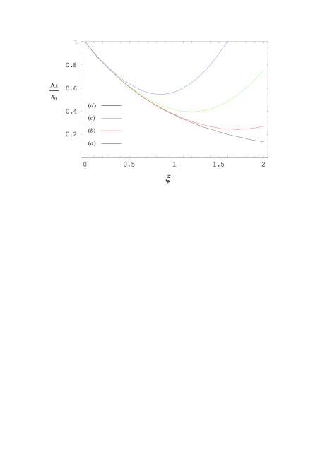
Figure 2: (Color online) Squeezed efficiency $\Delta x/x_{0}$ versus $\xi$ for different ratios (a) $D/2\kappa\beta=0$, (b) $D/2\kappa\beta=0.001$, (c) $D/2\kappa\beta=0.01$, (d) $D/2\kappa\beta=0.05$.

For the linewidth $D$, and in the limit $D\ll\tau^{-1}\ll 2\kappa\beta$, the variances in the two quadratures are given by scully

$$\Delta x=x_{0}\sqrt{e^{-2\xi}+(\frac{D\tau}{2})e^{2\xi}},$$ (18a)

$$\Delta p=p_{0}e^{\xi}\sqrt{1-2D\tau}.$$ (18b)

In Fig.2, we have plotted $\Delta x/x_{0}$ versus $\xi$ for various ratios of $D/2\kappa\beta$. The variances in the amplitude of $x$ increases due to the phase fluctuations in the driving coherent state. There is a minimum in $\Delta x/x_{0}$ which decreases with increasing $D/2\kappa\beta$. It’s evident from Eq.(18a) that the phase fluctuation in driving coherent state would affect the squeezed efficient severely with increasing time $\tau$ due to the existence of $e^{2\xi}$.

IV discussion and conclusion

Our scheme is much different from the existing ones such as Refs.moon ; zhou ; rabl ; tian ; Ruskov . In our scheme, it doesn’t need any operations on the CPB and doesn’t use dissipation and measurement to generate the needed nonlinearity. It just needs to adiabatically keep the CPB in it’s ground state. Our scheme can greatly decrease the effect of the decoherence of the CPB on the squeezed efficency. The CPB plays the role of nonlinear media as in quantum optics, and our result is similar to the three-wave mixing. By controlling $n_{g}>1/2$ and/or $N_{g}<1/2$, we can get different squeezed variables $x$ and/or $p$.

In conclusion, we proposed a scheme for generating squeezed states in solid state circuits system. In such a system, a NMR is fabricated as a part of a SQUID, which consists of a CPB, and a STLR is capacitively coupled to the CPB. The nonlinear interaction between the CPB and the NMR can be implemented by setting the external biased flux of the CPB at some certain values. By performing Fröhlich transformation, we can get the nonlinear Hamiltonian of parametric down-conversion of the STLR-NMR system. In our scheme, the CPB plays the role of “nonlinear media” and the squeezed states of the NMR can be generated in a manner similar to the three-wave mixing in quantum optics.

- (1) A. Gaidarzhy, G. Zolfagharkhani, R. L. Badzey and P. Mohanty, Phys. Rev. Lett. 94, 030402 (2005);
- (2) M. O. Scully and M. S. Zubairy, Quantum Optics, Cambridge University Press, Cambridge, 1997.
- (3) M. F. Bocko and R. Onofrio, Rev. Mod. Phys. 68, 755 (1996).
- (4) R. E. Slusher, L. W. Hollberg, B. Yurke, J. C. Mertz, and J. F. Valley, Phys. Rev. Lett. 55, 2409 (1985).
- (5) L. A. Wu, H. J. Kimble, J. L. Hall and H. Wu, Phys. Rev. Lett. bf 57, 2520 (1987).
- (6) N. G. de Almeida, R. M. Serra, C. J. Villas-Böas and M. H. Y. Moussa, Phys. Rev. A 69, 035802 (2004).
- (7) A. Blais, R.-S. Huang, A. Wallraff, S. M. Girvin, and R. J. Schoelkopf, Phys. Rev. A 69, 062320 (2004).
- (8) I. Chiorescu, P. Bertet, K. Semba, Y. Nakamura, C. J. P. M. Harmans and J. E. Mooij, Nature 431, 159 (2004).
- (9) A. N. Cleland and M. R. Geller, Phys. Rev. Lett. 93, 070501 (2004).
- (10) W. Y. Huo and G. L. Long, arXiv:quant-ph/0702104.
- (11) A. Wallraff, D. I. Schuster, A. Blais, L. Frunzio, R.- S. Huang, J. Majer, S. Kumar, S. M. Girvin, and R. J. Schoelkopf, Nature 431, 162 (2004).
- (12) M. R. Geller and A. N. Cleland, Phys. Rev. A 71, 032311 (2005).
- (13) K. Moon and S. M. Girvin, Phys. Rev. Lett. 95, 140504 (2005).
- (14) X. X. Zhou and A. Mizel, Phys. Rev. Lett.97, 267201 (2006).
- (15) P. Rabl, A. Shnirman and P. Zoller, Phys. Rev. B 70, 205304 (2004).
- (16) L. Tian and R. W. Simmonds, arXiv: cond-mat/0606787.
- (17) R. Ruskov, K. Schwab and A. N. Korotkov, Phys. Rev. B 71, 235407 (2005).
- (18) F. Xue, Y. X. Liu, C. P. Sun and F. Nori, arXiv: quant-ph/0701209.
- (19) G. Benivegna and A. Messina, J. Mod. Opt. 41, 907 (1994).
- (20) Y. B. Xie, J. Mod. Opt. 42, 2239 (1994).
- (21) C. P. Sun, L. F. Wei, Y. X. Liu, and F. Nori, Phys. Rev. A 73, 022318 (2006).
- (22) Y. Makhlin, G. Schön and A. Shnirman, Rev. Mod. Phys. 73, 357 (2001).
- (23) A. D. Armour, M. P. Blencowe and K. C. Schwab, Phys. Rev. Lett. 88, 148301 (2002).
- (24) E. K. Irish and K. Schwab, Phys. Rev. B 68, 155311 (2003).
- (25) I. Martin, A. Shnirman, L. Tian and P. Zoller, Phys. Rev. B 69,125339 (2004).
- (26) H. Frhlich, Phys. Rev. 79, 845 (1950).