PROBING THE STRUCTURE OF GAMMA-RAY BURST JETS WITH THE STEEP DECAY PHASE OF THEIR EARLY X-RAY AFTERGLOWS

Abstract

We show that the jet structure of gamma-ray bursts(GRBs) can be investigated with the tail emission of the prompt GRB. The tail emission that we consider is identified as a steep decay component of the early X-ray afterglow observed by the X-Ray Telescope on board Swift. Using a Monte Carlo method, we derive for the first time the distribution of the decay index of the GRB tail emission for various jet models. The new definitions of the zero of time and the time interval of a fitting region are proposed. These definitions for fitting the light curve lead us to a unique definition of the decay index, which is useful to investigate the structure of the GRB jet. We find that if the GRB jet has a core-envelope structure, the predicted distribution of the decay index of the tail has a wide scatter and multiple peaks, which cannot be seen for the case of the uniform- and the Gaussian jet. Therefore, the decay index distribution gives us information about the jet structure. Especially if we observe events whose decay index is less than about 2, both the uniform- and the Gaussian jet models will be disfavored, according to our simulation study.

1 Introduction

Gamma-ray burst (GRB) jet structure, that is, the energy distribution $E(\theta)$ in the ultra-relativistic collimated outflow, is at present not yet fully understood (Zhang & Mészáros, 2002b). There are many jet models proposed in addition to the simplest uniform-jet model: the power-law jet model (Rossi et al., 2002; Zhang & Mészáros, 2002a), the Gaussian jet model (Zhang et al., 2004), the annular jet model (Eichler & Levinson, 2004), the multiple emitting subshell model (Kumar & Piran, 2000; Nakamura, 2000), the two-component jet model (Berger et al., 2003), and so on. The jet structure may depend on the generation process of the jet and therefore may provide us important information about the central engine of the GRB. For example, in the collapsar model for long GRBs (e.g., Zhang et al., 2003, 2004), the jet penetrates into and breaks out of the progenitor star, resulting in the $E(\theta)\propto\theta^{-2}$ profile (Lazzati & Begelman, 2005). For the compact binary merger model for short GRBs, hydrodynamic simulations have shown that the resulting jet tends to have a flat core surrounded by the power-law-like envelope (Aloy et al., 2005).

In the pre-Swift era, there were many attempts to constrain the GRB jet structure. Thanks to the HETE-2, statistical properties of long GRBs, X-ray-rich GRBs, and X-ray flashes were obtained (Sakamoto et al., 2005), which were thought to constrain the jet models (Lamb et al., 2004). These observational results constrain various jet models, such as the uniform-jet model (Yamazaki et al., 2004a; Lamb et al., 2005; Donaghy, 2006), the multiple subshell model (Toma et al., 2005b), the Gaussian jet model (Dai & Zhang, 2005), and so on. For BATSE long GRBs, Yonetoku et al. (2005) derived the distribution of the pseudo-opening angle, inferred from the Ghirlanda (Ghirlanda et al., 2004) and Yonetoku (Yonetoku et al., 2004) relations, as $f(\theta_{j})d\theta_{j}\propto\theta_{j}^{-2}d\theta_{j}$, which is compatible with that predicted by the power-law jet model as discussed in Perna et al. (2003) (however, see Nakar et al., 2004). Afterglow properties are also expected to constrain the jet structure (e.g., Granot & Kumar, 2003); however, energy redistribution effects prevent us from reaching a definite conclusion. Polarization measurements of optical afterglows bring us important information (Lazzati et al., 2004).

In the Swift era, rapid follow-up observation reveals prompt GRBs followed by a steep decay phase in the X-ray early afterglow (Tagliaferri et al., 2005; Nousek et al., 2006; O’Brien et al., 2006a). In the most popular interpretations, the steep decay component is the tail emission of the prompt GRB (the so called high-latitude emission), i.e., the internal shock origin (Zhang et al., 2006; Yamazaki et al., 2006; Liang et al., 2006; Dyks et al., 2005), although there are some other possibilities (e.g., Kobayashi et al., 2007; Panaitescu et al., 2006; Pe’er et al., 2006; Lazzati & Begelman, 2006; Dado et al., 2006). Then, for the uniform-jet case, the predicted decay index is $\alpha=1-\beta$, where we use the convention $F_{\nu}\propto T^{-\alpha}\nu^{1+\beta}$ (Kumar & Panaitescu, 2000). For power-law jet case ($E(\theta)\propto\theta^{-q}$), the relation is modified to $\alpha=1-\beta+(q/2)$. However, these simple analytical relations cannot be directly compared with observations, because they are for the case in which the observer’s line of sight is along the jet axis and because changing the zero of time, which potentially lies anywhere within the epoch where we see the bright pulses, substantially alters the early decay slope.

Recently, Yamazaki et al. (2006) (Y06) investigated the tail emission of the prompt GRB, finding that the jet structure can be described and that the global decay slope is not so much affected by the local angular inhomogeneity as it is affected by the global energy distribution. They also argued that the structured jet model is preferable, because steepening GRB tail breaks appeared in some events. In this paper, we calculate for the first time the distribution of the decay index of the prompt tail emission for various jet models and find that the derived distributions can be distinguished from each other, so that the jet structure can be more directly constrained than previous arguments. This paper is organized as follows. We describe our model in § 2. In § 3, we investigate the distribution of the decay index of the prompt GRB emission. Section 4 is devoted to discussions.

2 Tail Part of the Prompt GRB Emission

We consider the same model as discussed in the previous works (Y06; Yamazaki et al., 2004b; Toma et al., 2005a, b). The whole GRB jet, whose opening half-angle is $\Delta\theta_{{{\rm tot}}}$, consists of $N_{{{\rm tot}}}$ emitting subshells. We introduce the spherical coordinate system $(r,\vartheta,\varphi,t)$ in the central engine frame, where the origin is at the central engine and $\vartheta=0$ is the axis of the whole jet. Each emitting subshell departs at time $t_{{{\rm dep}}}^{{\scriptscriptstyle(j)}}$ ($0<t_{{{\rm dep}}}^{{\scriptscriptstyle(j)}}<t_{{{\rm dur}}}$, where $j=1,\cdots,N_{{{\rm tot}}}$, and $t_{{{\rm dur}}}$ is the active time of the central engine) from the central engine in the direction of $\vec{n}^{{\scriptscriptstyle(j)}}=(\vartheta^{{\scriptscriptstyle(j)}},\varphi^{{\scriptscriptstyle(j)}})$, and emits high-energy photons, generating a single pulse as observed. The direction of the observer is denoted by $\vec{n}_{\rm obs}=(\vartheta_{{{\rm obs}}},\varphi_{{{\rm obs}}})$. The observed flux from the $j$th subshell is calculated when the following parameters are determined: the viewing angle of the subshell $\theta_{v}^{{\scriptscriptstyle(j)}}=\cos^{-1}(\vec{n}_{{{\rm obs}}}\cdot\vec{n}^{{\scriptscriptstyle(j)}})$, the angular radius of the emitting shell $\Delta\theta_{{{\rm sub}}}^{{\scriptscriptstyle(j)}}$, the departure time $t_{{{\rm dep}}}^{{\scriptscriptstyle(j)}}$, the Lorentz factor $\gamma^{{\scriptscriptstyle(j)}}=(1-\beta_{\scriptscriptstyle(j)}^{2})^{-1/2}$, the emitting radius $r_{0}^{{\scriptscriptstyle(j)}}$, the low- and high-energy photon indices $\alpha_{B}^{{\scriptscriptstyle(j)}}$ and $\beta_{B}^{{\scriptscriptstyle(j)}}$, the break frequency in the shell comoving frame ${\nu^{\prime}_{0}}^{{\scriptscriptstyle(j)}}$ (Band et al., 1993), the normalization constant of the emissivity $A^{{\scriptscriptstyle(j)}}$, and the source redshift $z$. The observer time $T=0$ is chosen as the time of arrival at the observer of a photon emitted at the origin $r=0$ at $t=0$. Then, at the observer, the starting and ending times of the $j$th subshell emission are given by

$$T_{\rm start}^{\scriptscriptstyle(j)} \sim t_{{{\rm dep}}}^{\scriptscriptstyle(j)}+\frac{r_{0}^{\scriptscriptstyle(j)}}{2c\gamma_{\scriptscriptstyle(j)}^{2}}\left(1+\gamma_{\scriptscriptstyle(j)}^{2}{\theta_{-}^{\scriptscriptstyle(j)}}^{2}\right)~{}~{},$$ (1)

$$T_{\rm end}^{\scriptscriptstyle(j)} \sim t_{{\rm dep}}^{\scriptscriptstyle(j)}+\frac{r_{0}^{\scriptscriptstyle(j)}}{2c\gamma_{\scriptscriptstyle(j)}^{2}}\left(1+\gamma_{\scriptscriptstyle(j)}^{2}{\theta_{+}^{\scriptscriptstyle(j)}}^{2}\right)~{}~{},$$ (2)

where $\theta_{+}^{\scriptscriptstyle(j)}=\theta_{v}^{\scriptscriptstyle(j)}+\Delta\theta_{{\rm sub}}^{\scriptscriptstyle(j)}$, $\theta_{-}^{\scriptscriptstyle(j)}={\rm max}\{0,\theta_{v}^{\scriptscriptstyle(j)}-\Delta\theta_{{\rm sub}}^{\scriptscriptstyle(j)}\}$, and we use the formulas $\beta_{\scriptscriptstyle(j)}\sim 1-1/2\gamma_{\scriptscriptstyle(j)}^{2}$ and $\cos\theta\sim 1-\theta^{2}/2$ for $\gamma^{\scriptscriptstyle(j)}\gg 1$ and $\theta\ll 1$, respectively. The whole light curve from the GRB jet is produced by the superposition of the subshell emission.

Y06 discussed some kinematical properties of prompt GRBs in our model and found that each emitting subshell with $\theta_{v}^{\scriptscriptstyle(j)}\gg\Delta\theta_{{\rm sub}}^{\scriptscriptstyle(j)}$ produces a single, smooth, long-duration, dim, and soft pulse, and that such pulses overlap with each other and make the tail emission of the prompt GRB. Local inhomogeneities in the model are almost averaged during the tail emission phase, and the decay index of the tail is determined by the global jet structure, that is the mean angular distribution of the emitting subshell because in this paper all subshells are assumed to have the same properties unless otherwise stated. Therefore, we are essentially studying the tail emission from the usual continuous jets at once, i.e., from uniform- or power-law jets with no local inhomogeneity. In the following, we study various energy distributions of the GRB jet through the change of the angular distribution of the emitting subshell.

3 Decay Index of the Prompt Tail Emission

In this section, we perform Monte Carlo simulations in order to investigate the jet structure by calculating the statistical properties of the decay index of the tail emission. For a fixed-jet model, we randomly generate $10^{4}$ observers with their line of sights (LOSs) $\vec{n}_{\rm obs}=(\vartheta_{{{\rm obs}}},\varphi_{{{\rm obs}}})$. For each LOS, the light curve, $F(T)$ of the prompt GRB tail in the 15–25 keV band is calculated, and the decay index is determined. The adopted observation band is the low-energy end of the Burst Alert Telescope(BAT) detector and near the high-energy end of the X-Ray Telescope(XRT) on Swift. Hence, one can observationally obtain continuous light curves, beginning with the prompt GRB phase to the subsequent early afterglow phase (Sakamoto et al., 2007), so that it is convenient for us to compare theoretical results with observations. However, our actual calculations have shown that our conclusion is not qualitatively altered, even if the observation band is changed, for example, to 0.5–10 keV, as usually considered for other references.

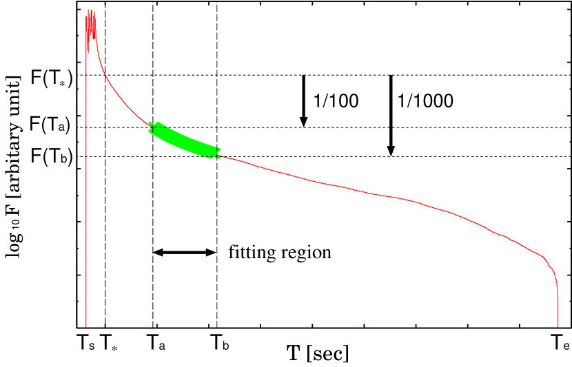
Figure 1: Example of how the decay index $\alpha$ is determined by the calculated light curve $F(T)$. The start and end time of the burst are denoted by $T_{\rm s}$ and $T_{\rm e}$, respectively. The time $T_{*}$ is determined by Eq. (5). The decay index $\alpha$ is determined by fitting $F(T)\propto(T-T_{*})^{-\alpha}$ in the time interval $[T_{a},T_{b}]$.

For each light curve, the decay index is calculated by fitting $F(T)$ with a single power-law form, $\propto(T-T_{*})^{-\alpha}$, as in the following (see Fig. 1). The decay index $\alpha$ depends on the choice of $T_{*}$ (Zhang et al., 2006; Yamazaki et al., 2006). Let $T_{\rm s}$ and $T_{\rm e}$ be the start and end time, respectively, of the prompt GRB, i.e.,

$$T_{\rm s} = {\rm min}\{T_{\rm start}^{\scriptscriptstyle(j)}\}$$ (3)

$$T_{\rm e} = {\rm max}\{T_{\rm end}^{\scriptscriptstyle(j)}\}~{}~{}.$$ (4)

Then, we take $T_{*}$ as the time until $99\%$ of the total fluence, which is defined by $S_{\rm total}=\int_{T_{\rm s}}^{T_{\rm e}}F(T^{\prime})~{}dT^{\prime}$, is radiated, that is,

$$\int_{T_{\rm s}}^{T_{*}}F(T^{\prime})~{}dT^{\prime}=0.99\,S_{\rm total}~{}~{}.$$ (5)

Then, the prompt GRB is in the main emission phase for $T<T_{*}$, while it is in the tail emission phase for $T>T_{*}$. The time interval $[T_{a},T_{b}]$, in which the decay index $\alpha$ is determined assuming the form $F(T)\propto(T-T_{*})^{-\alpha}$, is taken to satisfy

$$F(T_{a,b})=q_{a,b}F(T_{*})~{}~{},$$ (6)

where we adopt $q_{a}=1\times 10^{-2}$ and $q_{b}=1\times 10^{-3}$, unless otherwise stated. We find that in this epoch the assumed fitting form gives a well approximation.

At first, we consider the uniform-jet case, in which the number of subshells per unit solid angle is approximately given by $dN/d\Omega=N_{{\rm tot}}/(\pi\Delta\theta_{{\rm tot}}^{2})$ for $\vartheta<\Delta\theta_{{\rm tot}}$, where $\Delta\theta_{{\rm tot}}=0.25$ rad is adopted. The departure time of each subshell $t_{{{\rm dep}}}^{{\scriptscriptstyle(j)}}$ is assumed to be homogeneously random between $t=0$ and $t=t_{{{\rm dur}}}=20$ sec. The central engine is assumed to produce $N_{{{\rm tot}}}=1000$ subshells. In this section, we assume that all subshells have the same values of the following fiducial parameters: $\Delta\theta_{{{\rm sub}}}=0.02$ rad, $\gamma=100$, $r_{0}=6.0\times 10^{14}$ cm, $\alpha_{B}=-1.0$, $\beta_{B}=-2.3$, ${h\nu^{\prime}_{0}}=5$ keV, and $A={\rm constant}$. Our assumption of constant $A$ is justified as follows. Note that the case in which $N$ subshells that have the same brightness $A$ are launched into the same direction, but a different departure time, is equivalent to the case of one subshell emission with the brightness of $NA$. This is because in the tail emission phase, the second terms in the r.h.s. of Eqs. (1) and (2) dominate the first terms, so that the time difference effect, which arises from the difference of $t_{\rm dep}$ for each subshell, can be obscured. Hence, giving the angular distribution of the emission energy is equivalent to giving the angular distribution of the subshells with constant $A$. Also, Y06 showed that to obtain a smooth, monotonic tail emission as observed by Swift, the subshell properties, $h{\nu^{\prime}_{0}}^{{\scriptscriptstyle(j)}}$ and/or $A^{{\scriptscriptstyle(j)}}$, cannot have wide scatter in the GRB jet. Therefore, we can expect, at least as the zeroth-order approximation, that the subshells have the same properties.

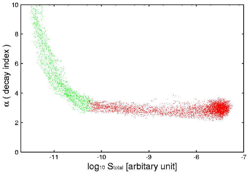
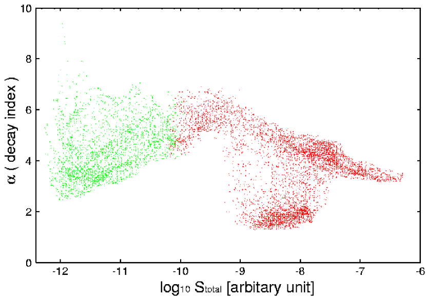
Figure 3: Decay index $\alpha$ as a function of the total fluence $S_{\rm total}$, the sum of the fluxes in the time interval $[T_{\rm s},T_{\rm e}]$. Red and green points represent events whose peak fluxes are larger and smaller than $10^{-4}$ times the largest one in all simulated events, respectively. Left and right panels are for the uniform- and power-law jet cases, respectively.

The left panel of Fig. 2 shows the decay index $\alpha$ as a function of $\vartheta_{\rm obs}$. For $\vartheta_{{{\rm obs}}}\lesssim\Delta\theta_{{{\rm tot}}}$ (on-axis case), $\alpha$ clusters around $\sim 3$. On the other hand, when $\vartheta_{{{\rm obs}}}\gtrsim\Delta\theta_{{{\rm tot}}}$ (off-axis case), $\alpha$ rapidly increases with $\vartheta_{\rm obs}$. The reason is as follows. If all subshells are seen sideways (that is, $\theta_{v}^{\scriptscriptstyle(j)}\gg\Delta\theta_{{\rm sub}}^{\scriptscriptstyle(j)}$ for all $j$), the bright pulses in the main emission phase followed by the tail emission disappear because of the relativistic beaming effect, resulting in a smaller flux contrast between the main emission phase and the tail emission phase compared with the on-axis case. Then $T_{*}$ becomes larger. Furthermore, in the off-axis case, the tail emission decays more slowly ($|dF/dT|$ is smaller) than in the on-axis case. Then both $T_{a}-T_{*}$ and $T_{b}-T_{*}$ are larger for the off-axis case than for the on-axis case. As can be seen in Fig. 3 of Zhang et al. (2006), the emission seems to decay rapidly, so that the decay index $\alpha$ becomes large. The left panel of Fig. 3 shows $\alpha$ as a function of the total fluence $S_{\rm total}$ which is the sum of the fluxes in the time interval, $[T_{\rm s},T_{\rm e}]$. In Fig. 3, both $\alpha$ and $S_{\rm total}$ are determined observationally, so that our theoretical calculation can be directly compared with the observation.

A more realistic model is the Gaussian jet model, in which the number of subshells per unit solid angle is approximately given by $dN/d\Omega=C\exp(-\vartheta^{2}/2\vartheta_{c}^{2})$ for $0\leqq\vartheta\leqq\Delta\theta_{{\rm tot}}$, where $C=N_{{\rm tot}}/2\pi\vartheta_{c}^{2}[1-\exp(-\Delta\theta_{{\rm tot}}^{2}/2\vartheta_{c}^{2})]$ is the normalization constant. We find only a slight difference between the results for the uniform- and the Gaussian jet models. Therefore, we do not show the results for the Gaussian jet case in this paper.

Next, we consider the power-law distribution. In this case, the number of subshells per unit solid angle is approximately given by $dN/d\Omega=C[1+(\vartheta/\vartheta_{c})^{2}]^{-1}$ for $0\leqq\vartheta\leqq\Delta\theta_{{\rm tot}}$, i.e., $dN/d\Omega\thickapprox C$ for $0\leqq\vartheta\ll\vartheta_{c}$ and $dN/d\Omega\thickapprox C(\vartheta/\vartheta_{c})^{-2}$ for $\vartheta_{c}\ll\vartheta\leqq\Delta\theta_{{\rm tot}}$, where $C=(N_{{\rm tot}}/\pi\vartheta_{c}^{2})[\ln(1+(\Delta\theta_{{\rm tot}}/\vartheta_{c})^{2})]^{-1}$ is the normalization constant and we adopt $\vartheta_{c}=0.02$ rad and $\Delta\theta_{{\rm tot}}=0.25$ rad. The other parameters are the same as for the uniform-jet case.

As can be seen in the right panels of Figs. 2 and 3, both the $\vartheta_{{\rm obs}}$–$\alpha$ and $S_{\rm total}$–$\alpha$ diagrams are complicated compared with the uniform-jet case. When $\vartheta_{{{\rm obs}}}\lesssim\vartheta_{c}$, the observer’s LOS is near the whole jet axis. Compared with the uniform-jet case, $\alpha$ is larger, because the power-law jet is dimmer in the outer region, i.e., emitting subshells are sparsely distributed near the periphery of the whole jet (see also the solid lines of Figs. 1 and 3 of Y06). If $\vartheta_{{{\rm obs}}}\gg\vartheta_{c}$, the scatter of $\alpha$ is large. Some bursts have an especially small $\alpha$ of around 2. This comes from the fact that the power-law jet has a core region ($0<\vartheta\lesssim\vartheta_{c}$), where emitting subshells densely distributed compared with the outer region. The core generates the light-curve break in the tail emission phase, as can be seen in Fig. 4 (Y06). In the epoch before the photons emitted by the core arrive at the observer (e.g., $T-T_{\rm s}\lesssim 7.5\times 10^{2}$ s for the solid line in Fig. 4), the number of subshells that contribute to the flux at time $T$, $N_{{\rm sub}}(T)$, increases with $T$ more rapidly than for the uniform-jet case. Then, the light curve shows a gradual decay. If the fitting region $[T_{a},\,T_{b}]$ lies in this epoch, the decay index $\alpha$ is around 2. In the epoch after the photons arising from the core are observed (e.g., $T-T_{\rm s}\gtrsim 7.5\times 10^{2}$ s for the solid line in Fig. 4), the subshell emission with $\theta_{v}^{\scriptscriptstyle(j)}\gtrsim\vartheta_{{\rm obs}}+\vartheta_{c}$ is observed. Then $N_{{\rm sub}}(T)$ rapidly decreases with $T$, and the observed flux suddenly drops. If the interval $[T_{a},\,T_{b}]$ lies in this epoch, the decay index becomes larger than 4.

To compare the two cases considered above more clearly, we derive the distribution of the decay index $\alpha$. Here we consider the events whose peak fluxes are larger than $10^{-4}$ times of the largest one in all simulated events, because the events with small peak fluxes are not observed. Fig. 5 shows the result. For the uniform-jet case (solid line), $\alpha$ clusters around 3, while for the power-law jet case (dotted line), the distribution is broad ($1\lesssim\alpha\lesssim 7$) and has multiple peaks.

So far, we have considered the fiducial parameters. In the following, we discuss the dependence on parameters, $r_{0}$, $\gamma$, $\beta_{B}$, $t_{\rm dur}$, and $\Delta\theta_{{\rm tot}}$ (It is found that the $\alpha$-distribution hardly depends on the value of $\alpha_{B}$, $\Delta\theta_{{\rm sub}}$, and $\nu^{\prime}_{0}$ within reasonable parameter ranges). At first, we consider the case in which $r_{0}=1.0\times 10^{14}$ cm is adopted, with other parameters being fiducial. Fig. 6 shows the result. The shape of the $\alpha$-distribution is almost the same as that for the fiducial parameters, in both the uniform- and the power-law jet cases. This comes from the fact that in a tail emission phase, the light curve for a given $r_{0}$ is approximately written as $F(T;r_{0})\thickapprox g(cT/r_{0})$, where a function $g$ determines the light-curve shape of the tail emission for other given parameters. Then, the light curves in the case of $r_{0}=r_{0,1}$ and $r_{0}=r_{0,2}$, namely, $F(T;r_{0,1})$ and $F(T;r_{0,2})$, satisfy the relation $F(T;r_{0,2})\thickapprox F((r_{0,1}/r_{0,2})T;r_{0,1})$. This can be seen, for example, by comparing the solid line with the dotted one in Fig. 4. Hence, $T_{*}$, $T_{a}$, and $T_{b}$ are approximately proportional to $r_{0}$; in this simple scaling, one can easily find that $\alpha$ remains unchanged for different values of $r_{0}$.

Second, we consider the case of $\gamma=200$ and $r_{0}=2.4\times 10^{15}$ cm, with other parameters being fiducial. In this case, the angular spreading timescale ($\propto r_{0}/\gamma^{2}$) is the same as in the fiducial case, so that the tail emissions still show smooth light curves, although the whole emission ends later, according to the scaling $T_{\rm e}\propto r_{0}$ (see the dot-dashed line in Fig. 4). Fig. 7 shows the result. For large $\gamma$, the relativistic beaming effect is more significant, so that the events in $\vartheta_{{{\rm obs}}}\gtrsim\Delta\theta_{{{\rm tot}}}$, which cause large $\alpha$, are dim compared with the small-$\gamma$ case. Such events cannot be observed. For the power-law jet case, therefore, the number of large-$\alpha$ events becomes small, although the distribution is still broad ($1\lesssim\alpha\lesssim 4$) and has two peaks. On the other hand, for the uniform-jet case, the distribution of the decay index $\alpha$ is almost the same as for the fiducial parameter set, because the value of the decay index $\alpha$ in the case of $\vartheta_{{{\rm obs}}}\lesssim\Delta\theta_{{{\rm tot}}}$ is almost the same as that in the case of $\vartheta_{{{\rm obs}}}\gtrsim\Delta\theta_{{{\rm tot}}}$.

Third, we change the value of the high-energy photon index $\beta_{B}$ from $-2.3$ to $-5.0$, with other parameters being fiducial. Fig. 8 shows the result. For the uniform-jet case, the mean value is $\langle\alpha\rangle\sim 4$, while $\langle\alpha\rangle\sim 3$ for the fiducial parameters, so that the decay index defined in this paper does not obey the well-known formula $\alpha=1-\beta_{B}$ (Kumar & Panaitescu, 2000). For the power-law jet case, the whole distribution shifts toward the higher value, and the ratio of the two peaks changes. In the tail emission phase, the spectral peak energy $E_{\rm peak}$ is below 15 keV (see also Y06), so that the steeper the spectral slope of the high-energy side of the Band function, the more rapidly the emission decays, resulting in the dimmer tail emission (see the dashed line in Fig. 4). Then, the fitting region $[T_{a},T_{b}]$ shifts toward earlier epochs, because $T_{*}$ becomes small. Therefore, the number of events with small $\alpha$ increases, and the number of events with large $\alpha$ decreases. Furthermore, we comment on the case in which $\beta_{B}$ is varied for each event in order to more directly compare with the observation. Here we randomly distribute $\beta_{B}$ according to the Gaussian distribution with a mean of $-2.3$ and a variance of $0.4$. It is found that the results are not qualitatively changed.

Next, we change the value of the duration time $t_{{\rm dur}}$ from $20$ sec to $200$ sec, with other parameters being fiducial. The epoch of the bright pulses in the main emission phase becomes longer than that in $t_{{\rm dur}}=20$ sec. However, the behavior of the tail emission does not depend on $t_{{\rm dur}}$ very much (see Fig. 9). Therefore, the distribution of the decay index $\alpha$ is almost the same as that for the fiducial parameters for both the uniform-jet case and the power-law jet case. Even if we consider the case in which $t_{\rm dur}$ is randomly distributed for each event according to the lognormal distribution with an average of $\log(20~{}{\rm s})$ and a logarithmic variance of $0.6$, the results are not significantly changed.

Finally, we discuss the dependence on $\Delta\theta_{{\rm tot}}$. Only the uniform-jet case is considered, because the structured jet is usually quasi-universal and because we focus our attention on the behavior of the uniform-jet model. The dotted line in Fig. 10 shows the result for constant $\Delta\theta_{{\rm tot}}=0.1$ rad with other parameters being fiducial. We can see many events with large $\alpha$. The large $\alpha$ is observed because for small $\Delta\theta_{\rm tot}$, although the off-axis events (i.e., $\Delta\theta_{\rm tot}\lesssim\vartheta_{\rm obs}$) are still dim because of the relativistic beaming effect, a fraction of such events survives the flux threshold condition and are observable. Such events have large $\alpha\gtrsim 5$ (see the 4th paragraph of this section, which explains the left panel of Fig. 2). This does not occur in the large-$\Delta\theta_{\rm tot}$ case. However, we still find in this case that there are no events with $\alpha\lesssim 2$. We consider another case in which $\Delta\theta_{{\rm tot}}$ is variable. Here we generate events whose $\Delta\theta_{{\rm tot}}$ distributes as $f_{\Delta\theta_{{\rm tot}}}d(\Delta\theta_{{\rm tot}})\propto\Delta\theta_{{\rm tot}}{}^{-2}d(\Delta\theta_{{\rm tot}})$ ($0.05\lesssim\Delta\theta_{{\rm tot}}\lesssim 0.4$). Then for a given $\Delta\theta_{{\rm tot}}$, the quantities $\nu^{\prime}_{0}$ and $A$ are determined by $h\nu^{\prime}_{0}=(\Delta\theta_{{\rm tot}}/0.13)^{-3.6}$ keV and $A\propto(\Delta\theta_{{\rm tot}})^{-7.3}$, respectively. Other parameters are fiducial. If the model parameters are chosen in this way, the Amati and Ghirlanda relations (Amati et al., 2002; Ghirlanda et al., 2004) are satisfied, and the event rates of long GRBs, X-ray-rich GRBs and X-ray flashes become similar (Donaghy, 2006). The solid line in Fig. 10 shows the result. Again we find that there are no events with $\alpha\lesssim 2$.

In summary, when we adopt model parameters within reasonable ranges, the decay index becomes larger than $\sim 2$ for the uniform- and the Gaussian jet cases, while a significant fraction of events with $\alpha\lesssim 2$ is expected for the power-law jet case. Therefore, if a non-negligible number of events with $\alpha\lesssim 2$ are observed, both the uniform- and the Gaussian jet models will be disfavored. Furthermore, if we observationally derive the $\alpha$-distribution, the structure of GRB jets will be more precisely determined.

4 Discussion

We have calculated the distribution of the decay index, $\alpha$, for the uniform-, Gaussian, and the power-law jet cases. For the uniform-jet case, $\alpha$ becomes larger than $\sim 2$, and its distribution has a single peak. The Gaussian jet model predicts almost the same results as the uniform-jet model. On the other hand, for the power-law jet case, $\alpha$ ranges between $\sim 1$ and $\sim 7$, and its distribution has multiple peaks. Therefore, we can determine the jet structure of GRBs by analyzing a lot of early X-ray data showing a steep decay component that is identified as a prompt GRB tail emission. However, one of the big challenges in the Swift data for calculating the decay index in our definition is to derive the composite light curve of BAT and XRT. Since the observed energy bands of BAT and XRT do not overlap, we are forced to extrapolate one of the data sets to plot the light curve in a given energy band. To derive the composite light curve unambiguously for a prompt and an early X-ray emission, we need an observation of a prompt emission by current instruments, which overlap the energy range of XRT.

The tail behavior with $\alpha\lesssim 2$ does not appear in the uniform- and the Gaussian jet models; hence, it is important to constrain the jet structure. However, in practical observations, such gradually decaying prompt tail emission might be misidentified with the external shock component, as expected in the pre-Swift era. Actually, some events have shown such a gradual decay, without the steep and the shallow decay phases, and their temporal and spectral indices are consistent with a classical afterglow interpretation (O’Brien et al., 2006b). Hence, in order to distinguish the prompt tail emission from the external shock component at a time interval $[T_{a},T_{b}]$, one should study the spectral evolution and/or the continuity and smoothness of the light curve (i.e., whether breaks appear or not) over the entire burst emission.

In this paper, we adopt $q_{a}=1\times 10^{-2}$ and $q_{b}=1\times 10^{-3}$ when the fitting epoch $[T_{a},T_{b}]$ is determined [see Eq. (6)]. Then, the prompt tail emission in this time interval is so dim that it may often be obscured by the external shock component, causing a subsequent shallow decay phase of the X-ray afterglow. One possible way to resolve this problem is to adopt larger values of $q_{a}$ and $q_{b}$, e.g., $q_{a}=1/30$ and $q_{b}=1\times 10^{-2}$, in which the interval $[T_{a},T_{b}]$ shifts toward earlier epochs, so that the flux then is almost always dominated by the prompt tail emission. We have calculated the decay index distribution for this case ($q_{a}=1/30$ and $q_{b}=1\times 10^{-2}$) and have found that the differences between uniform- and power-law jets still arises as can be seen in the case of $q_{a}=1\times 10^{-2}$ and $q_{b}=1\times 10^{-3}$, so that our conclusion remains unchanged. However, the duration of the interval, $T_{b}-T_{a}$, becomes short, which might prevent us from observationally fixing the decay index at high significance. If $q_{a}\gtrsim 1/30$, the emission at $[T_{a},T_{b}]$ is dominated by the last brightest pulse. Then, the light-curve shape at $[T_{a},T_{b}]$ does not reflect the global jet structure, but reflects the properties of the emitting subshell causing the last brightest pulse. Another way to resolve the problem is to remove the shallow decay component. For this purpose, the origin of the shallow decay phase should be clarified in order to extract the dim prompt tail emission exactly. The other problem is contamination of X-ray flares, whose contribution has to be removed in order to investigate the tail emission component. In any case, if the GRB occurs in an extremely low-density region (a so-called naked GRB), where the external shock emission is expected to be undetectable, our method may be a powerful tool to investigate the GRB jet structure.

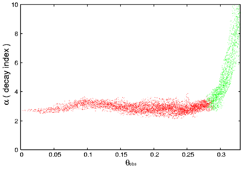
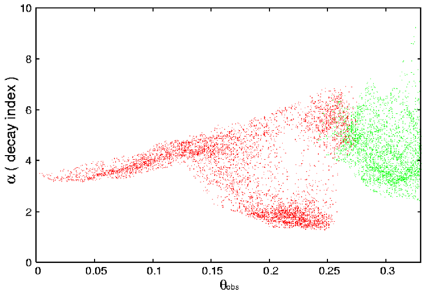
Figure 2: Decay index $\alpha$ as a function of $\vartheta_{\rm obs}$, the angle between the whole jet axis and the observers’ lines of sight. Red and green points represent events whose peak fluxes are larger and smaller than $10^{-4}$ times the largest one in all simulated events, respectively. Left and right panels are for the uniform- and power-law jet cases, respectively.

Figure 4: Examples of light curves of the prompt tail emission in the 15–25 keV band for the power-law jet case and $\vartheta_{\rm obs}>\vartheta_{c}$ ($\vartheta_{\rm obs}=0.27$ rad and $\vartheta_{c}=0.02$ rad). The solid line shows the fiducial parameters. A bump caused by the core emission can be seen at $T-T_{s}\sim 7.5\times 10^{2}$ s. The dotted, dot-dashed, and dashed lines are for $r_{0}=1.0\times 10^{14}$ cm; $r_{0}=2.4\times 10^{15}~{}cm$ and $\gamma=200$; and $\beta_{B}=-5$, respectively, with other parameters being fiducial. Time intervals $[T_{a},T_{b}]$ for each case are denoted by the thick solid lines. The flux is normalized by the peak value.

Figure 5: Distributions of the decay index $\alpha$ for uniform-jet ($dN/d\Omega=const.$;solid line) and power-law jet ($dN/d\Omega\propto[1+(\vartheta/\vartheta_{c})^{2}]^{-1}$;dotted line) models, respectively. We assume that all subshells have the same values of the following fiducial parameters: $\Delta\theta_{{{\rm sub}}}=0.02$ rad, $\gamma=100$, $r_{0}=6.0\times 10^{14}$ cm, $\alpha_{B}=-1.0$, $\beta_{B}=-2.3$, ${h\nu^{\prime}_{0}}=5$ keV, and $A={\rm constant}$. We consider events whose peak fluxes are larger than $10^{-4}$ times the largest one in all simulated events (red points in Fig. 2).

Figure 6: Same as Fig. 5, but for $r_{0}=1.0\times 10^{14}$ cm.

Figure 7: Same as Fig. 5, but for $\gamma=200$ and $r_{0}=2.4\times 10^{15}$ cm.

Figure 8: Same as Fig. 5, but for $\beta_{B}=-5.0$.

Figure 9: Same as Fig. 5, but for $t_{{\rm dur}}=200$ sec.

Figure 10: Distribution of the decay index $\alpha$ for the uniform-jet profile. The dotted line is for $\Delta\theta_{{\rm tot}}=0.1$ rad with other fiducial parameters. The solid line is for the variable-$\Delta\theta_{{\rm tot}}$ case, in which we generate events whose $\Delta\theta_{{\rm tot}}$ distributes as $f_{\Delta\theta_{{\rm tot}}}d(\Delta\theta_{{\rm tot}})\propto\Delta\theta_{{\rm tot}}{}^{-2}d(\Delta\theta_{{\rm tot}})$ ($0.05\lesssim\Delta\theta_{{\rm tot}}\lesssim 0.4$), and for given $\Delta\theta_{{\rm tot}}$, the quantities $\nu^{\prime}_{0}$ and $A$ are determined by $h\nu^{\prime}_{0}=(\Delta\theta_{{\rm tot}}/0.13)^{-3.6}$ keV and $A\propto(\Delta\theta_{{\rm tot}})^{-7.3}$, respectively. Other parameters are fiducial.

References

- Aloy et al. (2005) Aloy, M. A., Janka, H.-T., & Müller, E. 2005, A&A, 436, 273
- Amati et al. (2002) Amati, L., et al. 2002, A&A, 390, 81
- Band et al. (1993) Band, D. L., et al. 1993, ApJ, 413, 281
- Berger et al. (2003) Berger, E., et al., 2003, Nature, 426, 154
- Dado et al. (2006) Dado, S., Dar, A., & De Rujula, A. 2006, ApJ, 646, L21
- Dai & Zhang (2005) Dai, X. & Zhang, B. 2005, ApJ, 621, 875
- Donaghy (2006) Donaghy, T. Q. 2006, ApJ, 645, 436
- Dyks et al. (2005) Dyks, J., Zhang, B., & Fan, Y. Z. 2005, astro-ph/0511699
- Eichler & Levinson (2004) Eichler, D., & Levinson, A. 2004, ApJ, 614, L13
- Ghirlanda et al. (2004) Ghirlanda, G., Ghisellini, G., & Lazzati, D. 2004, ApJ, 616, 331
- Granot & Kumar (2003) Granot, J. & Kumar, P. 2003, ApJ, 591, 1086
- Kobayashi et al. (2007) Kobayashi, S. & Zhang, B. Mészáros, P., & Burrows, D., 2007, ApJ, 655, 391
- Kobayashi & Zhang (2007) Kobayashi, S. & Zhang, B. 2007, ApJ, 655, 973
- Kumar & Panaitescu (2000) Kumar, P. & Panaitescu, A. 2000, ApJ, 541, L51
- Kumar & Piran (2000) Kumar, P., & Piran, T. 2000, ApJ, 535, 152
- Lamb et al. (2004) Lamb, D. Q., et al. 2004, NewA Rev., 48, 423
- Lamb et al. (2005) Lamb, D. Q., Donaghy, T. Q., & Graziani, C. 2005, ApJ, 620, 355
- Lazzati et al. (2004) Lazzati, D., et al. 2004, A&A, 422, 121;
- Lazzati & Begelman (2005) Lazzati, D. & Begelman, M. C. 2005, ApJ, 629, 903
- Lazzati & Begelman (2006) Lazzati, D. & Begelman, M. C. 2006, ApJ, 641, 972;
- Liang et al. (2006) Liang, E. W., et al. 2006, ApJ, 646, 351
- Nakamura (2000) Nakamura, T. 2000, ApJ, 534, L159
- Nakar et al. (2004) Nakar, E., Granot, J., & Guetta, D. 2004, ApJ, 606, L37
- Nousek et al. (2006) Nousek, J. A., et al. 2006, ApJ, 642, 389
- O’Brien et al. (2006a) O’Brien, P. T., et al. 2006a, ApJ, 647, 1213
- O’Brien et al. (2006b) O’Brien, P. T., Willingale, R., Osborne, J. P., & Goad, M. R. 2006b, New J. Phys. 8, 121
- Panaitescu et al. (2006) Panaitescu, A., Mészáros, P., Gehrels, N., Burrows, D., & Nousek, J. 2006, MNRAS, 366, 1357
- Pe’er et al. (2006) Pe’er, A., Mészáros, P., Rees, M. J., 2006, ApJ, 652, 482
- Perna et al. (2003) Perna, R., Sari R., & Frail, D. 2003, ApJ, 594, 379
- Rossi et al. (2002) Rossi, E., Lazzati, D., & Rees, M. J. 2002, MNRAS, 332, 945
- Sakamoto et al. (2005) Sakamoto, T., et al. 2005, ApJ, 629, 311
- Sakamoto et al. (2007) Sakamoto, T., et al. 2007, submitted to ApJ
- Tagliaferri et al. (2005) Tagliaferri, G., et al. 2005, Nature, 436, 985
- Toma et al. (2005a) Toma, K., Yamazaki, R., & Nakamura, T. 2005a, ApJ, 620, 835
- Toma et al. (2005b) Toma, K., Yamazaki, R., & Nakamura, T. 2005b, ApJ, 635, 481
- Yamazaki et al. (2004a) Yamazaki, R., Ioka, K., & Nakamura, T. 2004a, ApJ, 606, L33
- Yamazaki et al. (2004b) Yamazaki, R., Ioka, K., & Nakamura, T. 2004b, ApJ, 607, L103
- Yamazaki et al. (2006) Yamazaki, R., Toma, K., Ioka, K., & Nakamura, T. 2006, MNRAS, 369, 311 (Y06)
- Yonetoku et al. (2004) Yonetoku, D., Murakami, T., Nakamura, T., Yamazaki, R., Inoue, A. K., & Ioka, K. 2004, ApJ, 609, 935
- Yonetoku et al. (2005) Yonetoku, D., Yamazaki, R., Nakamura, T., & Murakami, T. 2005, MNRAS, 362, 1114
- Zhang & Mészáros (2002a) Zhang, B., & Mészáros, P. 2002a, ApJ, 571, 876
- Zhang & Mészáros (2002b) Zhang, B., & Mészáros, P. 2002b, Int. J. Mod. Phys. A, 19, 2385
- Zhang et al. (2004) Zhang, B., Dai, X., Lloyd-Ronning, N. M., & Mészáros, P. 2004, ApJ, 601, L119
- Zhang et al. (2006) Zhang, B., et al. 2006, ApJ, 642, 354
- Zhang et al. (2003) Zhang, W., Woosley, S. E., & MacFadyen, A. I. 2003, ApJ, 586, 356
- Zhang et al. (2004) Zhang, W., Woosley, S. E., & Heger, A. 2004, ApJ, 608, 365