Black hole’s life at colliders

Abstract:

In the series of papers by Ida, Oda and Park, the complete description of Hawking radiation to the brane localized Standard Model fields from mini black holes in the low energy gravity scenarios are obtained. Here we briefly review what we have learned in those papers.

1 Introduction

We briefly review recent developments in the mini black hole production and evaporation mainly based on the series of works done by Ida, Oda and Park [1, 2, 3, 4]. In the low energy gravity scenarios such as ADD and RS-I, the CERN Large Hadronic collider (LHC) will become a black hole factory [5, 6]. Above the TeV Planck scale, the classical production cross section of the $(4+n)$-dimensional black hole grows geometrically $\sigma\sim\hat{s}^{1/(n+1)}$, with $\sqrt{\hat{s}}$ being the center of mass energy of the parton scattering.

Once produced, black hole loses its energy or mass primarily via Hawking (thermal) radiation. The Hawking radiation goes mainly into the standard model quarks and leptons (spinors) and gauge bosons (vectors) localized on the brane, except for a few gravitons and Higgs boson(s). The quanta of Hawking radiation will have characteristic energy spectrum determined by the Hawking temperature and the greybody factor. The process of Hawking radiation in four dimensional rotating black hole has been treated in detail by Teukolsky, Press, Page and others in 1970s’. In higher dimensions, however, it is shown that the process has quite different features.

• Hawking temperaure $T_{H}\propto(M_{bh})/M_{*})^{1/(n+1)}$ of a $(4+n)$ dimensional black hole is much higher than 4 dimensional one with the small fundamental scale $M_{*}\sim$ TeV $\ll M_{\rm Planck}$. With this high temperature, the number of available degrees of freedom for Hawking radiation are much bigger in $(4+n)$ dimensions with all the standard model particles localized on the brane [8].

• The near horizon geometry of $(4+n)$ dimensional black hole is quite complicated. Its geometry is different from that of a four dimensional Kerr black hole. With the highly modified geometry in the vicinity of the event horizon, frequency dependent correction factor of Hawking radiation, i.e., greybody factor, is also largely modified (also see the references [9, 10, 11] as independent studies on the same topic).

To understand the physics of those black holes, we have to understand the greybody factor of higher dimensional, rotating black hole [12, 13].

2 Generalized Teukolsky equation and greybody factor

The induced metric on the three-brane in the $(4+n)$-dimensional Myers-Perry solution [7] with a single nonzero angular momentum is given by

$$g = {\Delta-a^{2}\sin^{2}\vartheta\over\Sigma}dt^{2}+{2a(r^{2}+a^{2}-\Delta)\sin^{2}\vartheta\over\Sigma}dtd\varphi$$ (1)

$${}-{(r^{2}+a^{2})^{2}-\Delta a^{2}\sin^{2}\vartheta\over\Sigma}\sin^{2}\vartheta d\varphi^{2}-{\Sigma\over\Delta}dr^{2}-\Sigma d\vartheta^{2},$$

where

$$\Sigma=r^{2}+a^{2}\cos^{2}\vartheta,~{}~{}~{}\Delta=r^{2}+a^{2}-\mu r^{1-n}.$$ (2)

The parameters $\mu$ and $a$ are equivalent to the total mass $M$ and the angular momentum $J$

$$M={(2+n)A_{2+n}\mu\over 16\pi G_{4+n}},~{}~{}~{}J={A_{2+n}\mu a\over 8\pi G_{4+n}}$$ (3)

evaluated at the spatial infinity of the $(4+n)$-dimensional space-time, respectively, where $A_{2+n}=2\pi^{(3+n)/2}/\Gamma((3+n)/2)$ is the area of a unit $(2+n)$-sphere and $G_{4+n}$ is the $(4+n)$-dimensional Newton constant of gravitation.

1.Subtracting outgoing wave contamination at NH and separating ingoing and outgoing wave at FF are described. 2.Here we answer the question :what fraction of energy would be radiated into Hawking radiation in spin-down phase.

2.1 Asymptotic solutions in Kerr-Newman frame

We are given a linear, second-order equation, say

$$\frac{d^{2}R}{dr^{2}}+{\cal\eta}\frac{dR}{dr}+{\cal\tau}R=0,$$ (4)

where $\eta$ and $\tau$ are determined in Kerr-Newman frame as:

$$\eta = -\frac{(s-1)\Delta^{\prime}+2iK}{\Delta},$$ (5)

$$\tau = \frac{2i\omega r(2s-1)-\lambda}{\Delta}.$$ (6)

$$\Delta = r^{2}+a^{2}-(r_{H}^{2}+a^{2})\left(\frac{r_{H}}{r}\right)^{n-1},$$

$$K = (r^{2}+a^{2})w-ma.$$ (7)

The asymptotic solutions are given at NH and FF limits:

$$R^{\rm NH} \sim W_{\rm in}+W_{\rm out}e^{2ikr_{*}}\Delta^{s},$$ (8)

$$R^{\rm FF} \sim Y_{\rm in}r^{2s-1}+Y_{\rm out}e^{2ikr_{*}}/r.$$ (9)

2.2 BC: Subtracting outgoing contamination at NH

The solutions near the horizon $r\rightarrow r_{H}$ are

$$R^{\rm NH}_{\rm in} = 1+a_{1}(r-r_{H})+\frac{a_{2}}{2}(r-r_{H})^{2}+\cdots,$$

$$R^{\rm NH}_{\rm out} = e^{2ikr_{*}}(r-r_{H})^{s}\left(1+b_{1}(r-r_{H})+\cdots\right),$$ (10)

where the coefficients $a_{i}$’s and $b_{i}$’s are straightforward to compute:

$$a_{1} = -\frac{\tau_{-1}}{\eta_{-1}},$$ (11)

$$a_{2} = -\frac{(\eta_{0}+\tau_{-1})a_{1}+\tau_{0}}{1+\eta_{-1}},$$ (13)

$$\cdots,$$

where $\eta_{j}$ and $\tau_{j}$ are $j$-th order coefficients of Taylor expansion of $\eta$ and $\tau$, respectively.

For $s=1/2$ and $1$,

$$\tau_{-1} = \frac{2i\omega\delta_{s,1}-\lambda}{\Delta_{1}},$$ (14)

$$\tau_{0} = \lambda\frac{\Delta_{2}}{\Delta_{1}^{2}}+\delta_{s,1}\frac{2i\omega}{\Delta_{1}^{2}}(\Delta_{1}-\Delta_{2}),$$ (15)

$$\eta_{-1} = \frac{1}{2}\delta_{s,1/2}-2i\frac{K_{0}}{\Delta_{1}},$$ (16)

$$\eta_{0} = -\frac{2i}{\Delta_{1}^{2}}(K_{1}\Delta_{1}-K_{0}\Delta_{2}),$$ (17)

where

$$\Delta_{1} = 2+(n-1)(1+a^{2}),$$ (18)

$$\Delta_{2} = 1-n(n-1)(1+a^{2})/2,$$ (19)

$$K_{0} = (1+a^{2})\omega-am,$$ (20)

$$K_{1} = 2\omega.$$ (21)

The problem is to integrate Eq.4 from purely ingoing initial conditions at $r=r_{0}$ out to $r\rightarrow\infty$. Choosing the positive choice for $s$ makes $Y_{\rm in}$ stable and easily determined by an outward integration. However, for such an integration $R^{\rm NH}_{\rm out}$ is unstable against contaminating the purely ingoing solution. We can avoid the difficulty in mid-integration, relying on a mathematical transformation of the equation to stabilize the solutions in the two asymptotic regimes $r\rightarrow r_{H}$ and $r\rightarrow\infty$ as follows. To counteract the above contamination, let

$$\tilde{R}=R-(1+a_{1}(r-r_{H})).$$ (22)

Then $f$ satisfies the equation

$${\cal L}\tilde{R}=g,$$ (23)

where ${\cal L}=d^{2}/dr^{2}+\eta d/dr+\tau$ and $g=-{\cal L}\left(1+a_{1}(r-r_{H})\right)=-\eta a_{1}-\tau\left(1+a_{1}(r-r_{H})\right)$. Equation 23 is now stably integrated through both asymptotic regimes, i.e., from the near horizon to far field regimes.

Near the horizon, $\tilde{R}$ becomes

$$\tilde{R}(r\rightarrow r_{H}) = \frac{a_{2}}{2}(r-r_{H})^{2}+\cdots.$$ (24)

2.3 Separating solution at FF

For $s=1/2$,

$$R^{\rm FF}_{\rm in} \sim 1+\frac{c^{f}_{1}}{r}+\frac{c^{f}_{2}}{r^{2}}+\frac{c^{f}_{3}}{r^{3}}+\cdots,$$

$$R^{\rm FF}_{\rm out} \sim e^{2ikr_{*}}\frac{1}{r}(1+\frac{d^{f}_{1}}{r}+\frac{d^{f}_{2}}{r^{2}}\cdots),$$ (25)

where

$$c^{f}_{1} = -i\frac{\lambda}{2\omega},$$ (26)

$$\cdots$$ (27)

Then, $\tilde{R}_{1/2}$ becomes

$$\tilde{R}_{1/2}(r\rightarrow\infty)\simeq\left(Y_{\rm in}+1-a_{1}\right)+a_{1}r+\frac{Y_{\rm in}c^{f}_{1}}{r}+Y_{\rm out}\frac{e^{2i\omega r_{*}}}{r}.$$ (28)

Using this expression, we can easily read out $Y$’s without numerical difficulties.

Finally, the greybody factor could be written as

$$\Gamma_{s=1/2}=1-\frac{2\omega}{|c^{f}_{1}|}\frac{|Y_{\rm out}|^{2}}{|Y_{\rm in}|^{2}}.$$ (29)

For $s=1$,

$$R^{\rm FF}_{\rm in} \sim r(1+\frac{c^{v}_{1}}{r}+\frac{c^{v}_{2}}{r^{2}}+\frac{c^{v}_{3}}{r^{3}}+\cdots),$$

$$R^{\rm FF}_{\rm out} \sim e^{2ikr_{*}}\frac{1}{r}(1+\frac{d^{v}_{1}}{r}+\frac{d^{v}_{2}}{r^{2}}+\frac{d^{v}_{3}}{r^{3}}+\cdots),$$ (30)

where

$$c^{v}_{1} = -i\frac{\lambda}{2\omega},$$ (31)

$$c^{v}_{2} = -\frac{\lambda^{2}-4a\omega(a\omega-m)}{8\omega^{2}},$$

$$\cdots$$ .

Then, $\tilde{R}_{1}$ becomes

$$\tilde{R}_{1}(r\rightarrow\infty)\simeq\left(Y_{\rm in}-a_{1}\right)r+\left(Y_{\rm in}c^{v}_{1}-1+a_{1}\right)+\frac{Y_{\rm in}c^{v}_{2}}{r}+Y_{\rm out}\frac{e^{2i\omega r_{*}}}{r}.$$ (33)

Using this expression, we can easily read out $Y$’s without numerical difficulties.

Finally, the greybody factor could be written as

$$\Gamma_{s=1}=1-\frac{2\omega^{2}}{|c^{v}_{2}|}\frac{|Y_{\rm out}|^{2}}{|Y_{\rm in}|^{2}}.$$ (34)

3 Hawking radiations of mini-black hole

Schematically black hole evolution follows five successive steps as is depicted in Fig.1: the production phase, the balding phase, the spin-down phase, the Schwarzschild phase and the Planck phase. When a black hole is produced in high energy collision (production phase), the geometry is highly irregular, and could even be topologically non-trivial. By emitting (bulk) gravitons and other particles, the black hole will be settled down to a rotating black hole which is supposed to be well described by Myers-Perry solution in $(4+n)$ dimensional spacetime (balding phase).

The decay in spin-down and Schwarzschild phases are calculable in terms of Hawking radiation. We are interested in those phases (spin-down phase and Schwarzschild phase) and would answer what fraction of energy will be lost in each of these phases.

The rate of energy (and angular momentum) loss by Hawking radiation is given as follows:

$$-\frac{d}{dt}\left(\begin{array}[]{c}M\\ J\\ \end{array}\right)=\frac{1}{2\pi}\sum_{s,l,m}g_{s}\int_{0}^{\infty}d\omega\langle N_{s,l,m}\rangle\left(\begin{array}[]{c}\omega\\ m\\ \end{array}\right),$$ (39)

where $g_{s}$ is the number of “massless” degrees of freedom at temperature $T$, namely, the number of degrees of freedom whose masses are smaller than $T$, with spin $s$. The expected number of particles of the species of spin $s$ emitted in the mode with spheroidal harmonics $l$, axial angular momentum $m$ is

$$\langle N_{s,l,m}\rangle=\frac{{}_{s}\Gamma_{l,m}(a,\omega)}{e^{(\omega-m\Omega)/T}-(-1)^{2s}}.$$ (40)

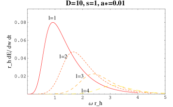
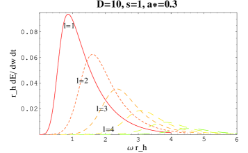
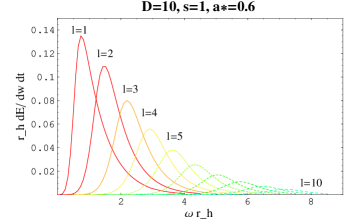
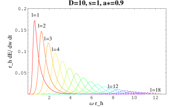
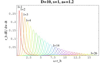
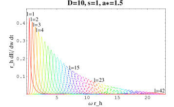
Figure 1: Hawking radiation from $D=10$ black hole. $s=1,a=0.01,0.3,0.6,0.9,1.2,1.5$.

4 Time evolution

From the ratio of energy and angular momentum in eq.39, we can define a scale invariant function $\gamma(a_{s}=a/r_{s})$ as follows:

$$\gamma^{-1}(a_{s}) \equiv \frac{d\ln a_{s}}{d\ln M}$$ (41)

$$= \frac{n+2}{2}\left(\frac{1}{a}\frac{dJ}{dM}-\frac{2}{n+1}\right).$$ (42)

Now we calculate the ratio of final($M_{f}$) and initial($M_{i}$) energy of black hole by integrating the eq.41 with $a_{s}({\rm ini})$ for initial angular momentum.

$$\frac{M_{f}}{M_{i}}={\rm Exp}\left(\int_{a_{s}(\rm ini)}^{a_{s}(\rm final)}da_{s}\frac{\gamma(a_{s})}{a_{s}}\right).$$ (43)

The amount of energy which is radiated in spin-down phase ($0\thickapprox a_{s}({\rm final})\leqslant a_{s}\leqslant a_{s}({\rm ini})$) is $(M_{i}-M_{f})$ and $M_{f}$ will be also radiated in Schwarzschild phase where the angular momentum of black hole is zero.

Next, let us consider the evolution of the black hole. Since time scales as $r_{s}^{n+3}$ in $(4+n)$ dimensions , it is convenient to introduce scale invariant rates for energy and angular momentum as follows.

$$\alpha(a_{s}) \equiv -r_{s}^{n+3}\frac{d\ln M}{dt},$$ (44)

$$\beta(a_{s}) \equiv -r_{s}^{n+3}\frac{d\ln J}{dt},$$ (45)

with these new variables $\gamma(a_{s})$ can be written as $\gamma^{-1}(a_{s})=\beta/\alpha(a_{s})-(n+2)/(n+1)$. We also introduce dimensionless variables $y$ and $z$ to take angular momentum and mass of the hole:

$$y \equiv -\ln a_{s},$$ (46)

$$z \equiv -\ln\frac{M}{M_{i}},$$ (47)

then finally we get the time variation of energy and angular momentum in terms of scale-invariant time parameter ($\tau=r_{s}^{-n-3}({\rm ini})t$) with initial mass of the hole:

$$\frac{dz}{dy} = \frac{\alpha}{\beta-\alpha\left(\frac{n+2}{n+1}\right)},$$

$$\frac{dy}{d\tau} = (\beta-\alpha\left(\frac{n+2}{n+1}\right))~{}e^{\frac{n+3}{n+1}z}.$$ (48)

After finding the solutions $z(y)$ and $\tau(y)$ of the coupled differential equations 48, one can get $y(\tau)$ and $z(\tau)$, hence $a_{s}$ and $M/M_{i}$, as a function of time. From these, one can find how other quantities evolve, such as the area.

Up to now we have used a unit where the size of event horizon is fixed as $r_{h}=1$ and angular momentum of the hole is parameterized by ($a_{h}=a/r_{h}$). For conversion of unit, the following expressions are useful with $a_{s}=a_{h}/(1+a_{h}^{2})^{1/(n+1)}$.

$$\alpha(a_{s}) = -\iota_{n}^{n+1}(1+a_{h}^{2})^{\frac{2}{n+1}}r_{h}^{2}\frac{dM}{dt},$$ (49)

$$\beta(a_{s}) = -\kappa_{n}^{n+1}(1+a_{h}^{2})^{\frac{2}{n+1}}r_{h}^{2}\frac{1}{a}\frac{dJ}{dt},$$ (50)

where

$$\iota_{n} = r_{s}M^{-\frac{1}{n+1}}=\left(\frac{16\pi G}{(n+2)\Omega_{n+2}}\right)^{\frac{1}{n+1}},$$ (51)

$$\kappa_{n} = \iota_{n}(\frac{n+2}{2})^{\frac{1}{n+1}}.$$ (52)

In Fig.2, black hole evolution in units of the initial mass as a function of rotation parameter $a_{s}$ for scalar(s), fermion(f), vector(v), and sum of all the standard model particles(SM) in $D=5$(left) and $D=10$ (right) are shown. The initial angular momentum parameter is fixed by $a_{s}=0.83$ and $2.67$ in $D=5$ and $D=10$ that are the maximal rotations allowed by the initial collision, respectively. The mass of the hole goes to zero before the rotation parameter goes to zero when only scalar emission is available. However, when all the standard model fields are turned on, the evolution is essentially determined by the spinor and vector radiation. It is found that a black hole spins down quickly at the first stage with large rotation parameter $a_{s}$ and the decrease of rotation parameter slows down as angular momentum of the hole is reduced.

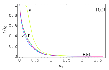
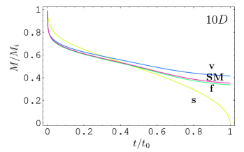
Figure 2: Evolution of bh in $D=10$.

When all the standard model fields are turned on (SM), the evolution is essentially determined by the spinor and vector radiation. The figures show that a black hole spins down quickly at the first stage with large rotation parameter and the decrease of rotation parameter slows down as angular momentum of the hole is reduced.

5 Summary and Discussion

The complete description of Hawking radiation to the brane localized SM fields and the consequent time evolution of mini black hole in the context of low energy gravity scenario has been made.

We have developed analytic and numerical methods to solve the radial Teukolsky equation which has been generalized to the higher dimension ($D=4+n$). Two main points in our numerical methods are as follows. First, we have imposed the proper purely-ingoing boundary condition near the horizon without the growing contamination of the out-going wave by extracting lower order terms explicitly. Second, we have developed the method to fit the in-going and out-going part from the numerically integrated wave solution at far field region by explicitly obtaining the next-to-next order expansion (or next-to-next-to-next order in vector case) of the solution. With these progress in numerical treatment, we can safely integrate the generalized Teukolsky equation up to very large $r$ without out-going wave contamination.

Then we have calculated all the possible modes to completely determine the radiation rate of the mass and angular momentum of the hole. Totally 3407 are computed explicitly, other than the modes which are confirmed to be negligible. A black hole tends to lose its angular momentum at the early stage of evolution. However the black hole still have a sizable rotating parameter after radiating half of its mass. More than $70\%$ or $80\%$ of black hole’s mass is lost during the spin down phase.

Now that we have completely determined the radiation and evolution of the spin-down and Schwarzschild phases, only remaining hurdle is the evaluation of the balding phase, which is still being disputed due to its non-purturbative nature, to extract the quantum gravitational information at the Planck phase from the experimental data at LHC.

References

• [1] D. Ida, K. y. Oda and S. C. Park, Phys. Rev.  D 67, 064025 (2003) [Erratum-ibid.  D 69, 049901 (2004)] [arXiv:hep-th/0212108].
• [2] D. Ida, K. y. Oda and S. C. Park, arXiv:hep-ph/0501210.
• [3] D. Ida, K. y. Oda and S. C. Park, Phys. Rev.  D 71, 124039 (2005) [arXiv:hep-th/0503052].
• [4] D. Ida, K. y. Oda and S. C. Park, Phys. Rev.  D 73, 124022 (2006) [arXiv:hep-th/0602188].
• [5] S. B. Giddings and S. D. Thomas, Phys. Rev.  D 65, 056010 (2002) [arXiv:hep-ph/0106219].
• [6] S. Dimopoulos and G. Landsberg, Phys. Rev. Lett.  87, 161602 (2001) [arXiv:hep-ph/0106295].
• [7] R. C. Myers and M. J. Perry, Annals Phys.  172, 304 (1986).
• [8] R. Emparan, G. T. Horowitz and R. C. Myers, Phys. Rev. Lett.  85, 499 (2000) [arXiv:hep-th/0003118].
• [9] C. M. Harris and P. Kanti, Phys. Lett.  B 633, 106 (2006) [arXiv:hep-th/0503010].
• [10] M. Casals, P. Kanti and E. Winstanley, JHEP 0602, 051 (2006) [arXiv:hep-th/0511163].
• [11] M. Casals, S. R. Dolan, P. Kanti and E. Winstanley, arXiv:hep-th/0608193.
• [12] S. C. Park and H. S. Song, J. Korean Phys. Soc.  43, 30 (2003) [arXiv:hep-ph/0111069].
• [13] S. C. Park, J. Korean Phys. Soc.  45, 208 (2004).