Singular Energy Distributions in Granular Media

Abstract

We study the kinetic theory of driven granular gases, taking into account both translational and rotational degrees of freedom. We obtain the high-energy tail of the stationary bivariate energy distribution, depending on the total energy $E$ and the ratio $x=\sqrt{E_{w}/E}$ of rotational energy $E_{w}$ to total energy. Extremely energetic particles have a unique and well-defined distribution $f(x)$ which has several remarkable features: $x$ is not uniformly distributed as in molecular gases; $f(x)$ is not smooth but has multiple singularities. The latter behavior is sensitive to material properties such as the collision parameters, the moment of inertia and the collision rate. Interestingly, there are preferred ratios of rotational-to-total energy. In general, $f(x)$ is strongly correlated with energy and the deviations from a uniform distribution grow with energy. We also solve for the energy distribution of freely cooling Maxwell Molecules and find qualitatively similar behavior.

I Introduction

Energy dissipation has profound consequences in granular materials, especially in dilute gases, where the dynamics are controlled by collisions bp ; pl ; pb . Dissipation is responsible for many interesting collective phenomena including clustering my ; ou ; lh ; nbc ; vvl , formation of shocks bcdr ; elm ; zbh ; rbss ; smk , and hydrodynamic instabilities gz ; km . Another consequence is the anomalous statistical physics that includes the non-Maxwellian velocity distributions lcdkg ; rm ; ao ; dlk ; kwg ; gzb and the breakdown of energy equipartition in mixtures wp ; fm .

For an elastic gas in equilibrium, the temperature, defined as the average kinetic energy, characterizes the entire distribution function including all of the moments, the bulk of the distribution, as well as the tail of the distribution. Outside of equilibrium, the temperature is not sufficient to characterize the energy distribution. Granular gases are inherently out of equilibrium and a complete characterization must therefore include the behavior of typical particles, the behavior of energetic particles, as well as the moments of the distribution. For example, the energy distribution may have power-law tails with divergent high-order moments kb ; eb ; bmp and consequently, the moments exhibit multiscaling bk . Generally, nonequilibrium effects are pronounced in the absence of energy input to balance the dissipation but can be suppressed by injection of energy where the deviation from a Maxwellian distribution affects only extremely energetic particles rm ; ve ; bk1 ; kssaob .

While there is substantial understanding of the energy distribution of frictionless granular gases, much less is known theoretically sz ; tg ; hz ; lhnz ; hhz ; jz ; hczhl ; hob and experimentally Walton ; flca ; trgl when the rotational degrees of freedom are taken into account. It is difficult to measure the rotational motion experimentally, and the few available measurements are restricted to two-dimensions. Surface roughness and friction have important consequences and the hydrodynamic theory jr ; bdks ; bdl ; ig must be modified, if the particles have spin gnb . Equipartition does not hold for the average rotational and translational temperature – neither in the free cooling case hz ; lhnz ; hhz ; jz nor for a driven system hczhl . In general, rotational and linear degrees of freedom are correlated in direction bpkz .

In this paper, we investigate the nature of the full energy distribution, that is, the bivariate distribution of rotational and translational energy. Motivated by the fact that on average the total energy is not partitioned equally between rotational and translational degrees of freedom, we focus on the bivariate distribution $P(E,x)$ of total energy $E$ and the modified ratio $x=\sqrt{E_{w}/E}$ of rotational to total energy. We thereby generalize the understanding of frictionless granular matter in terms of the energy distribution to rough grains.

Our starting point is the nonlinear Boltzmann equation with a collision rule that accounts for the coupling of translational and rotational motion due to tangential restitution. We study stationary solutions of the inelastic Boltzmann equation that describe steady states achieved through a balance between energy injections that are powerful but rare and energy dissipation through inelastic collisions. For high-energy particles we derive a linear equation for the bivariate energy distribution. The latter can be shown to factorize – $P(E,x)=p(E)f(x)$ – into a product of the distribution of the total energy, $p(E)$, and the distribution of the fraction of energy stored in the rotational degrees of freedom, $f(x)$. The former distribution decays algebraically with energy: $p(E)\sim E^{-\nu}$. The fraction of energy stored in rotational motion is universal for energetic particles in the sense that $f(x)$ approaches a limiting distribution independent of energy. Furthermore, this quantity has a number of interesting features. First, the distribution is not uniform, as it would be, if equipartition were to hold. Second, the distribution is not analytic but has singularities at special energy ratios. Third, the distribution and in particular its singularities depend sensitively on the moment of inertia and the collision parameters. Only for energetic particles is this distribution well defined. In general, the partition of energy into rotational and translational motion depends on the magnitude of the energy. This paper specifically addresses two-dimensions, although the theoretical approach and the reported qualitative behavior are generic.

We also develop a general framework for describing high-energy collisions and we use this framework to study freely cooling Maxwell Molecules where the moments of the energy distribution can be found in a closed form. For example, the two granular temperatures corresponding to the rotational and translational motions are coupled and generally, they are not equal. The high-energy behavior found for driven steady-states extends to freely cooling gases.

The rest of this paper is organized as follows. We review the collision rules and introduce the nonlinear kinetic theory in section II. We then derive the linear kinetic theory for high-energy particles in section III. Next, in section IV, we study driven steady states and solve for the stationary energy distribution. Freely cooling Maxwell molecules are discussed in section V and we conclude in section VI. The Appendices detail technical derivations.

II The Nonlinear Kinetic Theory

Our system consists of an infinite number of identical particles with mass $m=1$, radius $R$, and moment of inertia $I=qR^{2}$ where $0\leq q\leq 1$ is a dimensionless quantity. Each particle has a linear velocity ${\bf v}$ and an angular velocity ${\bf w}$. Its total energy is shared by the linear and the rotational motion, $E=E_{v}+E_{w}$, or explicitly,

$$E=\frac{1}{2}\left(v^{2}+qR^{2}w^{2}\right)$$ (1)

where $v\equiv|{\bf v}|$ and $w\equiv|{\bf w}|$.

In a collision between two particles, their velocities $({\bf v}_{i},{\bf w}_{i})$ with the labels $i=a,b$, change according to

$$({\bf v}_{a},{\bf w}_{a})+({\bf v}_{b},{\bf w}_{b})\to\ ({\bf v}^{\prime}_{a},{\bf w}^{\prime}_{a})+({\bf v}^{\prime}_{b},{\bf w}^{\prime}_{b})$$ (2)

where the postcollision velocities are denoted by primes. In a binary collision, rotational and translational energy are exchanged, while the total energy decreases. In this study, we consider tangential restitution in addition to the standard normal restitution. Let ${\bf r}_{i}$ be the position of particle $i$, then the directed unit vector connecting the centers of the colliding particles is $\hat{\bf n}=({\bf r}_{a}-{\bf r}_{b})/|{\bf r}_{a}-{\bf r}_{b}|$. We term this vector the impact direction. The collision rules are most transparent in terms of ${\bf u}_{i}$ the particle velocity at the contact point

$${\bf u}_{a} ={\bf v}_{a}+R\,\hat{\bf n}\times{\bf w}_{a}$$ (3a)

$${\bf u}_{b} ={\bf v}_{b}-R\,\hat{\bf n}\times{\bf w}_{b}.$$ (3b)

The inelastic collision laws state that the normal component of the relative velocity ${\bf U}={\bf u}_{a}-{\bf u}_{b}$ is reversed and reduced by the normal restitution coefficient $0\leq r_{n}\leq 1$. The tangential component is either reversed (rough particles) or not (smooth particles) and in any case reduced by the tangential restitution coefficient $-1\leq r_{t}\leq 1$, according to the following collision rules:

$${\bf U}^{\prime}\cdot\hat{\bf n} =-r_{n}{\bf U}\cdot\hat{\bf n},$$ (4a)

$${\bf U}^{\prime}\times\hat{\bf n} =-r_{t}\,{\bf U}\times\hat{\bf n}.$$ (4b)

Inelastic collisions conserve linear and angular momentum. Conservation of linear momentum implies that the total linear velocity does not change, and conservation of angular momentum enforces that the angular momentum of each particle with respect to the point of contact remains the same, because there is no torque acting at the point of contact. The collision laws (4) combined with these conservation laws specify the postcollision velocities as linear combinations of the precollision velocities hz

$${\bf v}_{a}^{\prime} ={\bf v}_{a}-\eta_{n}{\bf V}\cdot\hat{\bf n}\,\hat{\bf n}-\eta_{t}\left({\bf V}-{\bf V}\cdot\hat{\bf n}\,\hat{\bf n}\right)-\eta_{t}R\,\hat{\bf n}\times{\bf W}\qquad{\bf w}^{\prime}_{a}={\bf w}_{a}+\frac{\eta_{t}}{qR}\,\hat{\bf n}\times{\bf V}+\frac{\eta_{t}}{q}\,\hat{\bf n}\times\hat{\bf n}\times{\bf W}$$ (5a)

$${\bf v}_{b}^{\prime} ={\bf v}_{b}+\eta_{n}{\bf V}\cdot\hat{\bf n}\,\hat{\bf n}+\eta_{t}\left({\bf V}-{\bf V}\cdot\hat{\bf n}\,\hat{\bf n}\right)+\eta_{t}R\,\hat{\bf n}\times{\bf W}\qquad\,{\bf w}^{\prime}_{b}={\bf w}_{b}+\frac{\eta_{t}}{qR}\,\hat{\bf n}\times{\bf V}+\frac{\eta_{t}}{q}\,\hat{\bf n}\times\hat{\bf n}\times{\bf W}$$ (5b)

where the shorthand notations ${\bf V}={\bf v}_{a}-{\bf v}_{b}$ and ${\bf W}={\bf w}_{a}+{\bf w}_{b}$ were introduced. These collision rules involve the normal and tangential collision parameters, defined as

$$\eta_{n}=\frac{1+r_{n}}{2},\qquad{\rm and}\qquad\eta_{t}=\frac{q}{1+q}\frac{1+r_{t}}{2}.$$ (6)

Their range of values is bounded by $1/2\leq\eta_{n}\leq 1$ and $0\leq\eta_{t}\leq q/(1+q)$. Details of the derivation of the collision rules are given in Appendix A, as they are relevant for our discussion. The energy dissipation, $\Delta E=E_{a}+E_{b}-E_{a}^{\prime}-E_{b}^{\prime}$, is given by

$$\Delta E=\frac{1-r_{n}^{2}}{4}({\bf V}\cdot\hat{\bf n})^{2}+\frac{q}{1+q}\frac{1-r_{t}^{2}}{4}({\bf V}-{\bf V}\cdot\hat{\bf n}\,\hat{\bf n}+R\,\hat{\bf n}\times{\bf W})^{2}.$$ (7)

The energy dissipation is always positive, except when the collisions are elastic, $r_{n}=1$ and $r_{t}=-1$ (perfectly smooth spheres) or $r_{t}=1$ (perfectly rough spheres).

The collision rate $K({\bf v}_{a},{\bf v}_{b})$ is the rate by which the two particles approach each other. For hard spheres, this rate is simply the normal component of the relative velocity, but we study the general case

$$K({\bf v}_{a},{\bf v}_{b})=|({\bf v}_{a}-{\bf v}_{b})\cdot\hat{\bf n}|^{\gamma}$$ (8)

with $0\leq\gamma\leq 1$. Of course, the collision rate vanishes, $K=0$, when the particles are moving away from each other, $({\bf v}_{a}-{\bf v}_{b})\cdot\hat{\bf n}>0$. When particles interact via the central potential $r^{-\kappa}$ then $\gamma=1-2\frac{d-1}{\kappa}$ rd . The two limiting cases are hard spheres ($\gamma=1$) and Maxwell molecules ($\gamma=0$) where the collision rate is independent of the velocity jcm ; krupp ; tm ; mhe .

The central quantity in kinetic theory is the probability $P({\bf v},{\bf w},t)$ that a particle has the velocities $({\bf v},{\bf w})$ at time $t$. We study spatially homogeneous situations where this velocity distribution function is independent of position. Under the strong assumption that the velocities of the two colliding particles are completely uncorrelated, the velocity distribution obeys the Boltzmann equation

$$\frac{\partial P({\bf v},{\bf w})}{\partial t} = \frac{1}{2}\int d\hat{\bf n}\iiiint d{\bf v}_{a}d{\bf w}_{a}d{\bf v}_{b}d{\bf w}_{b}\,|({\bf v}_{a}-{\bf v}_{b})\cdot\hat{\bf n}|^{\gamma}\,P({\bf v}_{a},{\bf w}_{a})P({\bf v}_{b},{\bf w}_{b})$$

$$\times \big{[}\delta({\bf v}-{\bf v}_{a}^{\prime})\delta({\bf w}-{\bf w}_{a}^{\prime})+\delta({\bf v}-{\bf v}_{b}^{\prime})\delta({\bf w}-{\bf w}_{b}^{\prime})-\delta({\bf v}-{\bf v}_{a})\delta({\bf w}-{\bf w}_{a})-\delta({\bf v}-{\bf v}_{b})\delta({\bf w}-{\bf w}_{b})\big{]}.$$

We integrate over all impact directions with $\int d\hat{\bf n}=1$ condition and over the precollision velocities weighted by the respective probability distributions. There are two gain terms and two loss terms, because the velocities of interest $({\bf v},{\bf w})$ can be identified with any one of the four velocities in the collision rule (2) and the kernel is simply the collision rate (8).

III The Linear Kinetic Theory

The focus of this study is the energy distribution that generally depends only on two variables: $E_{v}$ and $E_{w}$. It is our aim to compute the distribution $P(E_{v},E_{w})$ for asymptotically large energies. This will be done for a system which is driven at very high energies as well as for an undriven system.

As a first step to this goal, we simplify the Boltzmann equation in the limit of large energies. Extremely energetic particles are rare and as a result it is unlikely that such particles will encounter each other. Hence, energetic particles typically collide with much slower particles. Since the collision rules are linear, the velocity of the slower particle barely affects the outcome of the collision. We can therefore neglect the slower velocity. Substituting $({\bf v}_{a},{\bf w}_{a})=({\bf v}_{0},{\bf w}_{0})$ and $({\bf v}_{b},{\bf w}_{b})=({\bf 0},{\bf 0})$ or $({\bf v}_{a},{\bf w}_{a})=({\bf 0},{\bf 0})$ and $({\bf v}_{b},{\bf w}_{b})=({\bf v}_{0},{\bf w}_{0})$ into (5) gives the cascade process bm ; bmm

$$({\bf v}_{0},{\bf w}_{0})\to({\bf v}_{1},{\bf w}_{1})+({\bf v}_{2},{\bf w}_{2})$$ (10)

where $({\bf v}_{0},{\bf w}_{0})$ is the precollision velocity of the energetic particle and $({\bf v}_{i},{\bf w}_{i})$ with $i=1,2$ are the consequent postcollision velocities. With these definitions, the collision rules for extremely energetic particles are

$${\bf v}_{1} =(1-\eta_{n}){\bf v}_{0}\cdot\hat{\bf n}\,\hat{\bf n}+(1-\eta_{t})({\bf v}_{0}-{\bf v}_{0}\cdot\hat{\bf n}\,\hat{\bf n})-\eta_{t}\hat{\bf n}\times{\bf w}_{0}\qquad{\bf w}_{1}=\left(1-\frac{\eta_{t}}{q}\right){\bf w}_{0}+\frac{\eta_{t}}{q}\hat{\bf n}\times{\bf v}_{0}$$ (11a)

$${\bf v}_{2} =\eta_{n}{\bf v}_{0}\cdot\hat{\bf n}\,\hat{\bf n}+\eta_{t}({\bf v}_{0}-{\bf v}_{0}\cdot\hat{\bf n}\,\hat{\bf n})+\eta_{t}\hat{\bf n}\times{\bf w}_{0}\quad\qquad\qquad\qquad\,{\bf w}_{2}=-\frac{\eta_{t}}{q}{\bf w}_{0}+\frac{\eta_{t}}{q}\hat{\bf n}\times{\bf v}_{0},$$ (11b)

where we have set $R=1$, so that the moment of inertia, $I=q$, is dimensionless. A collision between a high-energy particle and a typical-energy particle produces two energetic particles with an energy total that is smaller than the initial energy. This cascade process transfers energy from large scales to small scales.

Since the cascade process (10) involves only one particle, the tail of the probability distribution $P({\bf v},{\bf w})$ obeys the linear equation

$$\frac{\partial P({\bf v},{\bf w})}{\partial t}\!=\!\!\iiint d\hat{\bf n}d{\bf v}_{0}d{\bf w}_{0}|{\bf v}_{0}\cdot\hat{\bf n}|^{\gamma}P({\bf v}_{0},{\bf w}_{0})\big{[}\delta({\bf v}\!-\!{\bf v}_{1})\delta({\bf w}\!-\!{\bf w}_{1})\!+\!\delta({\bf v}\!-\!{\bf v}_{2})\delta({\bf w}\!-\!{\bf w}_{2})\!-\!\delta({\bf v}\!-\!{\bf v}_{0})\delta({\bf w}\!-\!{\bf w}_{0})\big{]}.$$ (12)

There are two gain terms and one loss term according to the cascade process (10). Formally, this linear rate equation can be obtained from the full nonlinear equation (II) by treating either one of the precollision velocities as negligible and then integrating over this small velocity. This procedure leads to four gain terms and two loss terms and thus, the factor $1/2$ in (II) drops out. We stress that the linear equation (12) is valid only in the high-energy limit.

We also comment that the linear equation (12) for the high-energy tail of the velocity distribution may be valid in cases where the full nonlinear equation is not. Whereas the nonlinear equation requires that all possible velocities are uncorrelated, the linear equation merely requires that energetic particles are uncorrelated with typical particles. This is a much weaker condition.

In this paper, we restrict ourselves to two space dimensions, i.e. rotating disks. In that case the rotational velocities are always perpendicular to the linear velocities. Thus, we conveniently denote the unit vector in the tangential direction by $\hat{\bf t}$ and the unit vector coming out of the plane by $\hat{\bf z}$, such that $\hat{\bf n}\cdot\hat{\bf t}=0$ and $\hat{\bf n}\times\hat{\bf t}=\hat{\bf z}$. The precollision velocities of the energetic particle ${\bf v}_{0}=v_{n}\,\hat{\bf n}+v_{t}\,\hat{\bf t}$ and ${\bf w}_{0}=w\,\hat{\bf z}$ are compactly written as $[v_{n},v_{t},w]$. With this notation, the postcollision velocities specified in (12) are

$$\Big{[}(1-\eta_{n})v_{n},(1-\eta_{t})v_{t}+\eta_{t}w,(\eta_{t}/q)v_{t}+(1-\eta_{t}/q)w\Big{]},\qquad{\rm and}\qquad\Big{[}\eta_{n}v_{n},\eta_{t}(v_{t}-w),(\eta_{t}/q)(v_{t}-w)\Big{]},$$ (13)

respectively. We now treat the three velocity components, namely the normal component of the velocity $v_{n}$, the tangential component of the velocity $v_{t}$, and the scaled angular velocity $\sqrt{q}w$ as a three dimensional vector with magnitude $V_{0}$, polar angle $\theta_{0}$, and azimuthal angle $\phi_{0}$:

$$(v_{n},v_{t},\sqrt{q}w)=(V_{0}\sin\theta_{0}\cos\phi_{0},V_{0}\sin\theta_{0}\sin\phi_{0},V_{0}\cos\theta_{0}).$$ (14)

The magnitude $V_{0}$ gives the energy $E_{0}=\frac{1}{2}V_{0}^{2}=\frac{1}{2}(v_{n}^{2}+v_{t}^{2}+qw^{2})$ while the polar angle characterizes the fraction of energy stored in the rotational degree of freedom, $\frac{1}{2}qw^{2}/E_{0}=\cos^{2}\theta$. In this representation, the postcollision velocities are three-dimensional vectors with magnitude $V_{i}$, polar angle $0\leq\theta_{i}\leq\pi$, and azimuthal angle $0\leq\phi_{i}\leq 2\pi$. The collision rules (11) allow us to express these quantities in terms of $V_{0},\theta_{0},\phi_{0}$:

$$(V_{i}\sin\theta_{i}\cos\phi_{i},V_{i}\sin\theta_{i}\sin\phi_{i},V_{i}\cos\theta_{i})=(V_{0}A_{i},V_{0}B_{i},V_{0}C_{i})$$ (15)

where $i=1,2$. The magnitudes of the postcollision velocities are proportional to the magnitude of the precollision velocity. The three velocity components are scaled by three dimensionless constants $A_{i}$, $B_{i}$ and $C_{i}$, that depend on the angles $\theta_{0}$ and $\phi_{0}$ of the energetic particle, the collision parameters $\eta_{n}$ and $\eta_{t}$, and the moment of inertia $q$,

$$A_{1} =(1-\eta_{n})\sin\theta_{0}\cos\phi_{0}$$ (16a)

$$B_{1} =(1-\eta_{t})\sin\theta_{0}\sin\phi_{0}+(\eta_{t}/\sqrt{q})\cos\theta_{0}$$ (16b)

$$C_{1} =(\eta_{t}/\sqrt{q})\sin\theta_{0}\sin\phi_{0}+(1-\eta_{t}/q)\cos\theta_{0}$$ (16c)

$$A_{2} =\eta_{n}\sin\theta_{0}\cos\phi_{0}$$ (16d)

$$B_{2} =\eta_{t}\sin\theta_{0}\sin\phi_{0}-(\eta_{t}/\sqrt{q})\cos\theta_{0}$$ (16e)

$$C_{2} =(\eta_{t}/\sqrt{q})\sin\theta_{0}\sin\phi_{0}-(\eta_{t}/q)\cos\theta_{0}.$$ (16f)

The new energies are proportional to the precollision energies

$$E_{i}=\alpha_{i}E_{0},\qquad{\rm with}\qquad\alpha_{i}=A_{i}^{2}+B_{i}^{2}+C_{i}^{2}.$$ (17)

We term the parameters $0<\alpha_{i}<1$ the contraction parameters. Since the collisions are dissipative, these parameters satisfy the inequality $\alpha_{1}+\alpha_{2}\leq 1$. The equality $\alpha_{1}+\alpha_{2}=1$ holds only for elastic collisions ($r_{n}=|r_{t}|=1$). The energy dissipation is $\Delta E=E_{0}-E_{1}-E_{2}=\Lambda E$ with $\Lambda=1-\alpha_{1}-\alpha_{2}$ or explicitly,

$$\Lambda=\frac{1-r_{n}^{2}}{4}\sin^{2}\theta_{0}\cos^{2}\phi_{0}+\frac{q}{1+q}\frac{1-r_{t}^{2}}{4}\Big{(}\sin^{2}\theta_{0}\sin^{2}\phi_{0}+\frac{1}{q}\cos^{2}\theta_{0}\Big{)}.$$ (18)

The polar and azimuthal angles are given by

$$\cos\theta_{i}=\frac{C_{i}}{\sqrt{A_{i}^{2}+B_{i}^{2}+C_{i}^{2}}}\qquad{\rm and}\qquad\tan\phi_{i}=\frac{B_{i}}{A_{i}},$$ (19)

respectively.

Let us represent solid angles by $\Omega\equiv\cos\theta,\phi$. With this definition, the cascade process (11) is

$$(E_{0},\Omega_{0})\to(E_{1},\Omega_{1})+(E_{2},\Omega_{2})$$ (20)

with $E_{i}$ and $\Omega_{i}$ given by (17) and (19). Energetic particles have an important property: the solid angle is not coupled to the energy! Indeed, the postcollision angles depend only on the precollision angle. The cascade process has the following geometric interpretation: a three dimensional vector is duplicated into two vectors. Subsequently, these two vectors are scaled down by the contraction parameters (17), and rotated according to the angular transformation (19).

We can now write the linear Boltzmann equation for $P(E,\Omega)$, the distribution of energy and solid angle, in a closed form

$$\!\frac{\partial P(\!E,\!\Omega)}{\partial t}\!=\!\!\!\iint\!\!dE_{0}d\Omega_{0}\big{|}\!\sqrt{E_{0}}\!\sin\theta_{0}\!\cos\phi_{0}\!\big{|}^{\gamma}\!P(\!E_{0},\!\Omega_{0})\!\big{[}\delta(E\!-\!E_{1})\delta(\Omega\!-\!\Omega_{1})\!+\!\delta(E\!-\!E_{2})\delta(\Omega\!-\!\Omega_{2})\!-\!\delta(E\!-\!E_{0})\delta(\Omega\!-\!\Omega_{0})\big{]}.$$

Time was rescaled, $t\to 2^{\gamma/2}t$, to absorb the constant which arises from replacing velocity by energy in the collision rate (8). Henceforth, we implicitly assume that the distribution $P(E,\Omega)$ is independent of $\phi$ because the distribution of linear velocities must be isotropic. The integration over the energy is performed using the collision rule (17), leading to the linear rate equation for the tail of the energy distribution

$$\frac{\partial P(E,\Omega)}{\partial t}\!=\!E^{\gamma/2}\!\!\int d\Omega_{0}\big{|}\sin\theta_{0}\cos\phi_{0}\big{|}^{\gamma}\!\left[\!P\left(\!\frac{E}{\alpha_{1}},\Omega_{0}\!\right)\frac{\delta(\Omega-\Omega_{1})}{\alpha_{1}^{1+\gamma/2}}\!+\!P\left(\!\frac{E}{\alpha_{2}},\Omega_{0}\!\right)\frac{\delta(\Omega-\Omega_{2})}{\alpha_{2}^{1+\gamma/2}}\!-\!P(E,\Omega_{0})\delta(\Omega-\Omega_{0})\right].$$ (21)

This is a non-local equation as the density of particles with energy $E$ is coupled to the density of particles with the higher energies $E/\alpha_{1}$ and $E/\alpha_{2}$. We stress that this equation is a straightforward consequence of the cascade process (20) and that it can also be derived from the full nonlinear Boltzmann equation. Yet, there may be situations where the linear equation (21) is valid, while the nonlinear equation (II) is not valid. The bivariate energy distributions $P(E,\Omega)$ and $P(E_{v},E_{w})$ are completely equivalent but we analyze the former because the cascade process (20) is transparent in terms of the total energy and the solid angle.

IV Driven Steady-states

The inelastic Boltzmann equation admits stationary solutions for frictionless particles. These stationary solutions describe driven steady-states with rare but powerful injection of energy. The injected energy cascades from high-energies down to small energies, thereby balancing the energy lost in collisions. At energies below the injection scale, Eqs. (II), (12) and (21) are not altered by the energy source and consequently, the stationary solution of the inelastic Boltzmann equation holds up to this large energy scale bm ; bmm . Here, we seek a corresponding stationary solution for particles with rotational degrees of freedom in the high energy limit.

The stationary solution has to fulfill Eq. (21) with the left hand side set to zero

$$0=\int d\Omega_{0}\big{|}\sin\theta_{0}\cos\phi_{0}\big{|}^{\gamma}\!\left[\!\frac{1}{\alpha_{1}^{1+\gamma/2}}\!P\left(\!\frac{E}{\alpha_{1}},\Omega_{0}\!\right)\delta(\Omega-\Omega_{1})\!+\!\!\frac{1}{\alpha_{2}^{1+\gamma/2}}\!P\left(\!\frac{E}{\alpha_{2}},\Omega_{0}\!\right)\delta(\Omega-\Omega_{2})\!-\!P(E,\Omega_{0})\delta(\Omega-\Omega_{0})\right].$$ (22)

At high-energies, the solid angle is not coupled to the energy, as follows from Eq. (19). This fact has a major consequence: the bivariate energy distribution $P(E,\Omega)$ takes the form of a product of the energy distribution $p(E)=\int d\Omega\,P(E,\Omega)$ and the distribution of solid angle, $g(\Omega)$,

$$P(E,\Omega)\to p(E)\,g(\Omega)$$ (23)

as $E\to\infty$. The angle distribution is normalized, $\int d\Omega\,g(\Omega)=1$. It does not depend on the azimuthal angle, because on average the two components of the linear velocity are equivalent. Due to the equi-dimensional (in $E$) structure of the steady-state equation (22), the product ansatz (23) is a solution when the distribution $p(E)$ decays algebraically

$$p(E)\sim E^{-\nu},$$ (24)

as $E\to\infty$ bm ; bmm . We obtain a closed equation for the distribution $g(\Omega)$ by substituting the product ansatz (23) with the power-law form (24) into the steady-state equation (22)

$$0=\int d\Omega_{0}\,g(\Omega_{0})\,\big{|}\sin\theta_{0}\cos\phi_{0}\big{|}^{\gamma}\left[\alpha_{1}^{\nu-1-\gamma/2}\delta(\Omega-\Omega_{1})+\alpha_{2}^{\nu-1-\gamma/2}\delta(\Omega-\Omega_{2})-\delta(\Omega-\Omega_{0})\right].$$ (25)

This equation is linear in $g(\Omega)$. However, it is nonlinear in $\nu$ and moreover, the solid angles $\Omega_{i}\equiv\Omega_{i}(\Omega_{0})$ in (19) and the contraction parameters $\alpha_{i}\equiv\alpha_{i}(\Omega_{0})$ in (17) are complicated functions of the solid angle $\Omega_{0}$.

Equation (25) involves two unknowns quantities, the exponent $\nu$ and the distribution function $g(\Omega)$. A solution does not exist for arbitrary values of $\nu$. In fact, there is one and only one value of $\nu$ for which there is a solution for $g(\Omega)$. This is the value selected by the cascade dynamics! In other words, (25) is an eigenvalue equation: $\nu$ is the eigenvalue and $g(\Omega)$ is the eigenfunction. This eigenvalue equation circumvents the full nonlinear equation (II) and thus, represents a significant simplification.

The physical interpretation of (25) involves a cascade process in which the solid angle undergoes a creation-annihilation process

$$\Omega_{0}\to\begin{cases}\emptyset&{\rm with\ rate\ }\beta_{0},\\ \Omega_{1}&{\rm with\ rate\ }\beta_{1},\\ \Omega_{2}&{\rm with\ rate\ }\beta_{2}.\end{cases}$$ (26)

Here, $\beta_{i}=|\sin\theta_{0}\cos\phi_{0}\big{|}^{\gamma}\alpha_{i}$ for $i=0,1,2$ and $\alpha_{0}=1$. There is one annihilation process and two creation processes. These processes have relative weights that reflect the powerlaw decay of $p(E)$. At the steady-state, the creation and the annihilation terms balance (see Appendix B), as reflected in the integrated form of (25)

$$0=\int d\Omega_{0}\,g(\Omega_{0})\big{|}\sin\theta_{0}\cos\phi_{0}\big{|}^{\gamma}\left[\alpha_{1}^{\nu-1-\gamma/2}+\alpha_{2}^{\nu-1-\gamma/2}-1\right].$$ (27)

To achieve a steady-state, $\beta_{i}<\beta_{0}$ for $i=1,2$ and therefore $\alpha_{i}^{\nu-1-\gamma/2}<1$. Since $\alpha_{i}<1$, we have the lower bound $\nu>1+\gamma/2$.

We can immediately check that for elastic collisions, $\nu=2+\gamma/2$ avb ; asb because $\alpha_{1}+\alpha_{2}=1$, and therefore, we conclude the bounds $1+\gamma/2\leq\nu\leq 2+\gamma/2$. The exponent $\nu$ varies continuously with the restitution coefficients $r_{n}$ and $r_{t}$ and the normalized moment of inertia $q$. This quantity must coincide with the value found for frictionless particles where tangential restitution is irrelevant ($r_{t}=-1$) bm ; bmm ; relate , but otherwise the exponent is distinct, as shown in Fig. 1. Also, the exponent $\nu$ increases monotonically with $r_{n}$ and $|r_{t}|$. We conclude that the rotational degrees of motion do affect the power-law behavior (24).

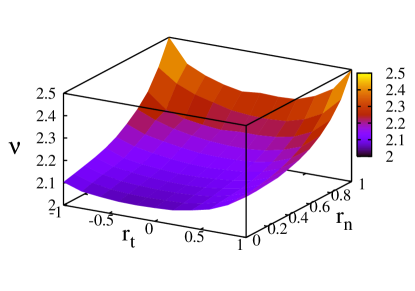
Figure 1: The exponent $\nu$ for hard spheres ($\gamma=1$) as a function of the coefficients of normal, $r_{n}$, and tangential, $r_{t}$, restitution coefficients. The numerical procedure for solving (25) is detailed below.

The azimuthal angle $\theta$ characterizes the fraction of energy stored in the rotational mode, $\cos^{2}\theta=E_{w}/E$ with $E_{w}=\frac{1}{2}qw^{2}$. The angle distribution $g(\Omega)=(2\pi)^{-1}\tilde{f}(\cos\theta)$ therefore captures the partition of energy into rotational and translational energies. We introduce the natural variable $0\leq x\leq 1$ defined by $x=|\cos\theta|$ so that

$$x=\sqrt{\frac{E_{w}}{E}}$$ (28)

and present results for the angle distribution $f(x)=2\tilde{f}(\cos\theta)$. In equilibrium, energy is partitioned equally into all degrees of freedom and therefore $g_{\rm eq}(\Omega)=(4\pi)^{-1}$ or equivalently,

$$f_{\rm eq}(x)=1$$ (29)

for $0\leq x\leq 1$. In particular, $\langle x^{2}\rangle=1/3$.

IV.1 Simulation Methods

We numerically studied the angle distribution $f(x)$ by solving the linear eigenvalue equation (25) for the “angular” process (26) and by solving the full nonlinear Boltzmann equation (II) for the collision process (2). Both of these equations are solved using Monte Carlo simulations.

The eigenvalue equation is solved by mimicking the angular process. Throughout the simulation, the value $\nu$ is fixed. There are $N$ particles, each with a given polar angle. A particle with polar angle $\theta_{0}$ is picked at random and then, a random azimuthal angle $\phi_{0}$ is drawn. The polar angles $\theta_{1}$ and $\theta_{2}$ are then calculated according to (19). The original particle is annihilated with probability $\beta_{0}$ and simultaneously, a new particle with angle $\theta_{1}$ is created with probability $\beta_{1}$ and similarly, a second particle with angle $\theta_{2}$ is created with probability $\beta_{2}$. Therefore, the number of particles may increase by one, remain unchanged, or decrease by one. The exponent $\nu$ is the value that keeps the total number of particles constant in the long time limit. The eigenvalue $\nu$ is calculated by repeating this simulation for various values of $\nu$ and then using the bisection method ptvf . We present Monte Carlo simulations of $100$ independent realizations with $N=10^{7}$ particles.

Driven steady-states are obtained by simulating the two competing processes of inelastic collisions and energy injection. In an inelastic collision, two particles are picked at random and also, the impact direction is chosen at random. The particle velocities are updated according to the collision law (5). Collisions are executed with probability proportional to the collision rate. Throughout this process, we keep track of the total energy loss. With a small rate, we augment the energy of a randomly selected particle by an amount equal to the loss total and subsequently, reset the total energy loss to zero. A fraction of the injected energy is rotational and the complementary fraction is translational. We draw this fraction according to the equilibrium distribution (29). We experimented with different angle distributions and found that the resulting stationary state did not change.

Obtaining the distribution $f(x)$ is generally challenging as it requires excellent statistics. The simulations are most efficient for Maxwell molecules because all possible collisions are equally likely. Therefore, for the full nonlinear Boltzmann equation (II), we present the angle distribution of the energetic particles only for the case $\gamma=0$.

For Maxwell molecules, the injection rate is $10^{-4}$ and the system size is $N=10^{7}$. The corresponding values for hard spheres are $10^{-2}$ and $N=10^{5}$. In all cases, the simulation results represent an average over $10^{2}$ independent realizations. Unless noted otherwise, the simulation results are for maximally dissipative ($r_{n}=r_{t}=0$) disks ($q=1/2$).

IV.2 The Distribution of Total Energy

The numerical simulations confirm several of our theoretical predictions. First, the energy distribution approaches a steady-state with a power-law high-energy tail. Second, the distribution of the total energy $p(E)$ decays algebraically as in (24). Third, the exponent $\nu$ is in excellent agreement with the predictions of the eigenvalue equation. For Maxwell molecules, Monte Carlo simulation of the full nonlinear equation yields $\nu=1.570\pm 0.005$ whereas numerical solution of the eigenvalue equation (25) gives $\nu=1.569\pm 0.005$ (Fig. 3). For hard-spheres, where the simulation results are slightly less accurate, the corresponding values are $\nu=2.065\pm 0.005$ and $\nu=2.060\pm 0.005$ (Fig. 3). The behavior of the distribution of total energy is therefore qualitatively similar to the behavior in the no-rotation case bm ; bmm . However, the quantitative behavior is different because the exponent $\nu$ does depend on the tangential restitution coefficient and the moment of inertia (Fig. 1).

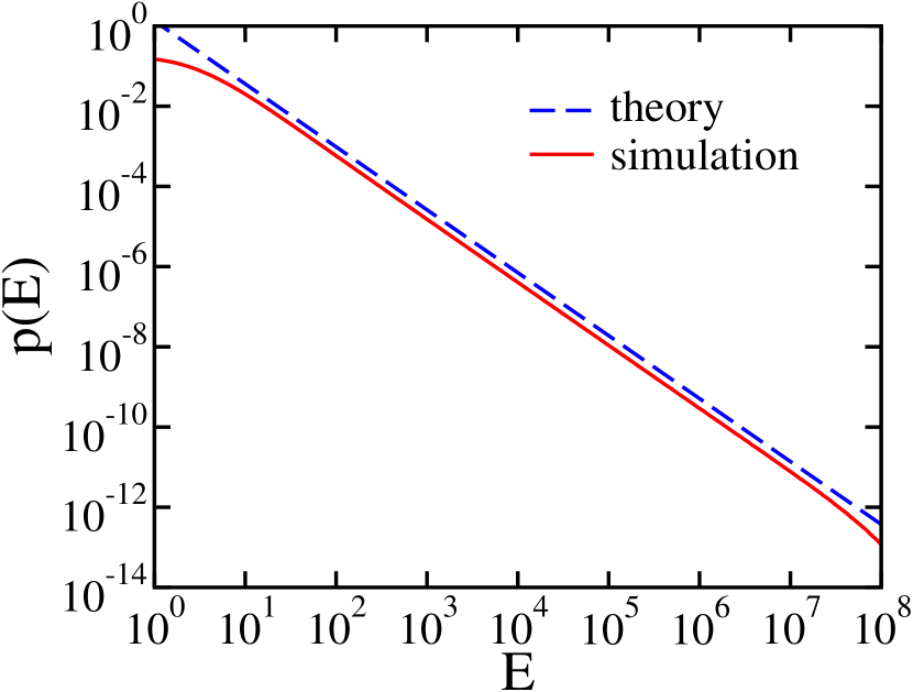
Figure 2: The tail of the energy distribution for driven Maxwell molecules. Shown are simulation results (solid line) and a line with the slope predicted by the theory (dashed line). The energy is normalized by the typical energy $10^{-4}$.

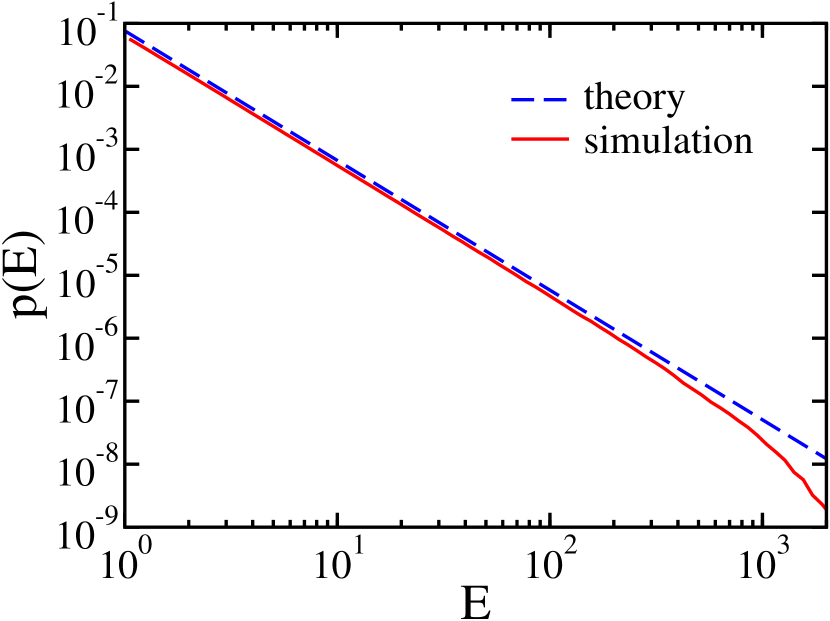
Figure 3: The tail of the energy distribution for driven hard spheres. Shown are simulation results (solid line) and a line with the slope predicted by the theory (dashed line).

IV.3 The Angle distribution

The numerical simulations also confirm several of our theoretical predictions concerning the angle distribution. Extremely energetic particles have a universal distribution $f(x)$. This distribution is independent of the energy, provided that the energy is sufficiently large. We had to probe only the most energetic particle out of roughly $10^{3}$ particles to measure this distribution. For this reason, the linear analysis and the resulting eigenvalue equation are valuable because they allow for an accurate and efficient determination of the angle distribution of the energetic particles. We also verified that the distribution $f(x)$ obeys the eigenvalue equation (25), as demonstrated in Fig. 5, where the simulations are compared to the solution of the angular process.

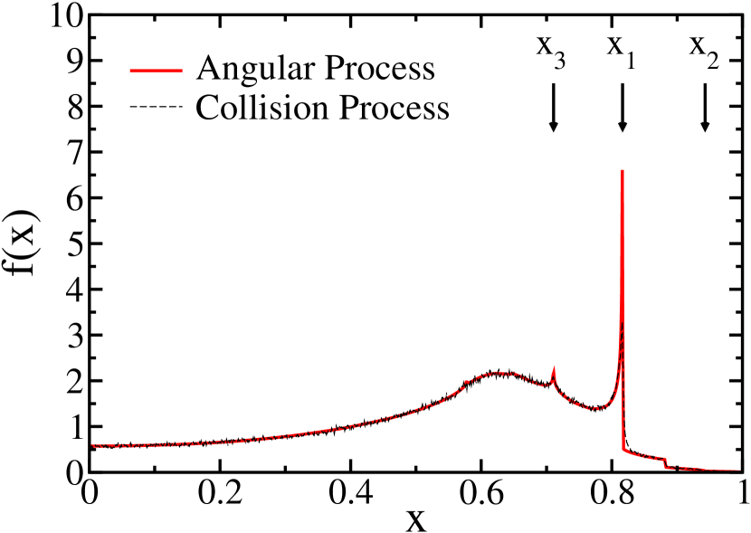
Figure 4: The angle distribution $f(x)$ obtained by Monte Carlo simulation of the angular process (26) (solid line) and the collision process (2) (dashed line) for Maxwell molecules. The special values $x_{1}$, $x_{2}$, and $x_{3}$ discusses in the text are indicated by arrows.

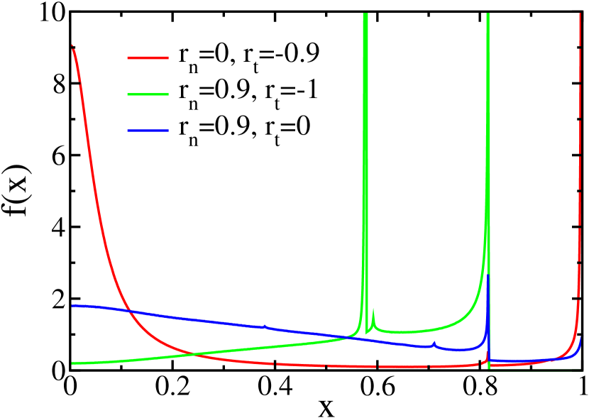
Figure 5: The angle distribution $f(x)$ for various collision parameters ($r_{n}$ and $r_{t}$) for Maxwell molecules.

The distribution $f(x)$ has several noteworthy features. First, it is not uniform, implying the breakdown of energy equipartition in a granular gas. Furthermore, this distribution is nonanalytic. It contains singularities and discontinuous derivatives. There are notable peaks in the distribution so that special values $x$ and special ratios $E_{w}/E$ are strongly preferred. The reason for these peaks is the fact that the polar angle is limited. For example, $\cos^{2}\theta_{2}<1/(1+q)$ as seen by substituting $\cos\theta_{0}=\pm 1$ into (16) and (19). Consequently, there is a special ratio

$$x_{1}=\sqrt{\frac{1}{1+q}}$$ (30)

with the corresponding special energy ratio $E_{w}/E=x_{1}^{2}$. This is the most pronounced peak in Fig. 5, $x_{1}=\sqrt{2/3}=0.81649$. Numerically, we observe that the peak becomes more pronounced as the distribution is measured at a finer scale, indicating that the distribution function diverges at this point.

Similarly, there is another special ratio that corresponds to $\theta_{1}$ when $\cos\theta_{0}=\pm 1$, and unlike (30), this location depends on the tangential restitution,

$$x_{2}=\frac{1-\eta_{t}/q}{\sqrt{\eta_{t}^{2}/q+(1-\eta_{t}/q)^{2}}}.$$ (31)

Indeed, there is a barely noticeable cusp at $x_{2}=\sqrt{8/9}=0.942809$. Singularities may induce less pronounced “echo”-singularities. For example, using $\cos\theta_{0}=x_{1}$ and $\phi_{0}=\pi/2$ yields the special ratio

$$x_{3}=\frac{1+\eta_{t}(1-1/q)}{\sqrt{q[1-\eta_{t}(1-1/q)]^{2}+[1+\eta_{t}(1-1/q)]^{2}}}.$$ (32)

There is a noticeable peak at the corresponding value $x_{3}=\sqrt{50/99}=0.710669$ in Fig. 5. We anticipate that as the transformation (19) is iterated, the strength of the singularities weakens and as a result there are discontinuous derivatives of increasing order, a subtle behavior that is difficult to measure.

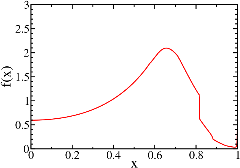
Figure 6: The angle distribution $f(x)$ for hard spheres.

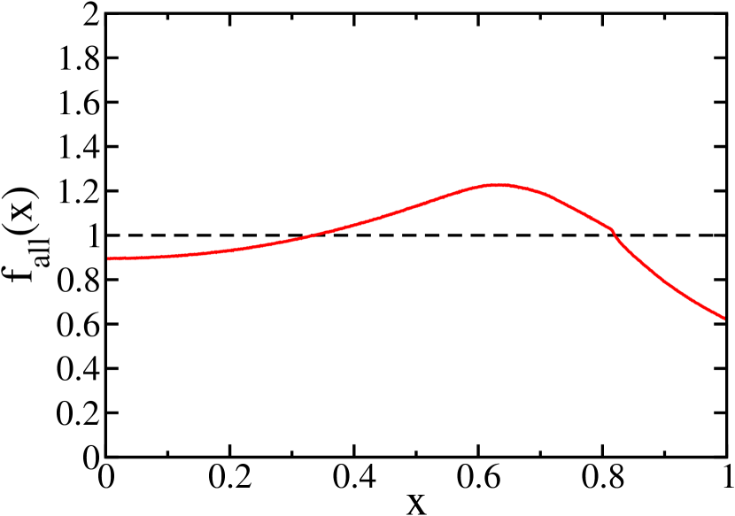
Figure 7: The angle distribution $f_{\rm all}(x)$ of all particles for Maxwell molecules (solid line). Also shown for reference is the uniform equilibrium distribution (broken line).

The location of the singularities varies with the collision parameters $r_{n}$ and $r_{t}$ and the moment of inertia $q$. In fact, the angle distribution is extremely sensitive to material properties as its shape changes dramatically with these parameters, see Fig. 5. The angle distribution also depends on the collision rate and it is much smoother for hard spheres, see Fig. 7. Since the collision rate vanishes for grazing collisions, $\phi=\pi/2$, the associated singularities including in particular (32) are suppressed. Nevertheless, there is a pronounced jump at the special ratio given by (30) and there are also noticeable cusps.

The angle distribution of all particles $f_{\rm all}(x)\propto\int dE\,P(E,\Omega)$ is shown in Fig. 7. It is substantially different from $f(x)$. Therefore, the energy distribution $P(E,\Omega)$ does not factorize in general and there are correlations between the solid angle and the total energy. Only for energetic particles does (23) hold. Moreover, $f_{\rm all}(x)$ is much smoother in comparison with $f(x)$ although there is a jump in the first derivative at the special ratio (30) showing that the angle distribution of all particles is also non-analytic, see Fig. 7. Generally, the angle distribution depends on energy and the deviation from a uniform distribution grows with energy.

We also comment that lone measurement of the moment $\langle x^{2}\rangle$ can be misleading. The angle distribution may very well have a value close to the equipartition value $\langle x^{2}\rangle_{\rm eq}=1/3$ but still, be very far from the equilibrium distribution. Indeed, in Fig. 5, $\langle x^{2}\rangle\cong 0.318$, a value that barely differs from the equilibrium value, even though the corresponding distribution is far from uniform. The second moment may also differ substantially from the equipartition value and for example, $\langle x^{2}\rangle=0.202$ when $r_{n}=0.9$ and $r_{t}=0$ (Fig. 5).

We argue that the qualitative features of the angle distribution should be generic in granular materials. Collisions involving energetic particles must follow the linear cascade rules (20) with the angular transformations (19). The singularities are a direct consequence of these transformations and therefore should be generic. Measuring the parameter-sensitive distribution $f(x)$ experimentally is challenging because a huge number of particles must be probed and the measurement has to be accurate. The distribution $f_{\rm all}(x)$ provides a detailed probe of the partition of energy into rotational and translation motion.

V Free Cooling

We now consider freely cooling granular gases that evolve via purely collisional dynamics. Without energy input, all energy is eventually dissipated and the particles come to rest. This system has been studied extensively bp for hard spheres with hz ; bpkz and without rotation ep .

We consider Maxwell molecules where in the absence of rotation an exact treatment is possible kb ; eb ; bk ; bcg ; bc . When $\gamma=0$ the Boltzmann equation (II) simplifies

$$\frac{\partial P({\bf v},{\bf w})}{\partial t} = \frac{1}{2}\int d\hat{\bf n}\iiiint d{\bf v}_{a}d{\bf w}_{a}d{\bf v}_{b}d{\bf w}_{b}\,P({\bf v}_{a},{\bf w}_{a})P({\bf v}_{b},{\bf w}_{b})$$

$$\times [\delta({\bf v}-{\bf v}_{a}^{\prime})\delta({\bf w}-{\bf w}_{a}^{\prime})+\delta({\bf v}-{\bf v}_{b}^{\prime})\delta({\bf w}-{\bf w}_{b}^{\prime})-\delta({\bf v}-{\bf v}_{a})\delta({\bf w}-{\bf w}_{a})-\delta({\bf v}-{\bf v}_{b})\delta({\bf w}-{\bf w}_{b})].$$

Consequently, the equations for the moments $\langle v^{n}w^{m}\rangle=\iint d{\bf v}d{\bf w}P({\bf v},{\bf w})v^{n}w^{m}$ close.

V.1 The Temperatures

Here, we consider only the translational temperature defined as the average translational energy, $T_{v}=\langle E_{v}\rangle$, and the rotational temperature, defined as the average rotational energy $T_{w}=\langle E_{w}\rangle$. These two temperatures are coupled through the linear equation

$$\frac{d}{dt}\left(\begin{array}[]{c}T_{v}\\ T_{w}\\ \end{array}\right)=-\left(\begin{array}[]{cc}\lambda_{vv}&\lambda_{vw}\\ \lambda_{wv}&\lambda_{ww}\\ \end{array}\right)\left(\begin{array}[]{c}T_{v}\\ T_{w}\\ \end{array}\right).$$ (34)

Appendix C details the derivation of the matrix of coefficients

$$\lambda_{vv} =\eta_{n}(1-\eta_{n})+\eta_{t}(1-\eta_{t})$$ (35a)

$$\lambda_{vw} =-2\eta_{t}^{2}/q$$ (35b)

$$\lambda_{wv} =-\eta_{t}^{2}/q$$ (35c)

$$\lambda_{ww} =2(\eta_{t}/q)(1-\eta_{t}/q).$$ (35d)

The two temperatures are coupled as long as $\eta_{t}\neq 0$ or alternatively, $r_{t}\neq-1$.

The solution of (34) is a linear combination of the two eigenvectors

$$\left(\begin{array}[]{c}T_{v}\\ T_{w}\\ \end{array}\right)=C_{-}\left(\begin{array}[]{c}1\\ c_{-}\\ \end{array}\right)e^{-\lambda_{-}t}+C_{+}\left(\begin{array}[]{c}1\\ c_{+}\\ \end{array}\right)e^{-\lambda_{+}t}$$ (36)

with the constants $C_{-}$ and $C_{+}$ set by the initial conditions, and $c_{\pm}=(\lambda_{\pm}-\lambda_{vv})/\lambda_{vw}$. The eigenvalues are

$$\lambda_{\pm}=\frac{\lambda_{vv}+\lambda_{ww}}{2}\pm\sqrt{\left(\frac{\lambda_{vv}-\lambda_{ww}}{2}\right)^{2}+\lambda_{vw}{\lambda_{wv}}}\,.$$ (37)

The larger eigenvalue is irrelevant in the long time limit and therefore,

$$\left(\begin{array}[]{c}T_{v}\\ T_{w}\\ \end{array}\right)\to C_{-}\left(\begin{array}[]{c}1\\ c_{-}\\ \end{array}\right)e^{-\lambda t}$$ (38)

such that both temperatures decay with the same rate $\lambda\equiv\lambda_{-}$. Of course, the total temperature also follows the same exponential decay, $T=T_{v}+T_{w}\sim e^{-\lambda t}$. In this regime, the fraction of rotational energy is on average

$$\lim_{t\to\infty}\frac{T_{w}}{T}=\frac{c_{-}}{1+c_{-}}=\frac{\lambda-\lambda_{vv}}{\lambda+\lambda_{vw}-\lambda_{vv}}.$$ (39)

The approach toward this value is exponentially fast and the relaxation time is inversely proportional to the difference in eigenvalues $\tau=1/(\lambda_{+}-\lambda_{-})$.

In equilibrium, $T_{w}/T=1/3$ but for nonequilibrium granular gases the ratio varies. In Fig. 8 we plot the ratio of the average rotational energy to the total energy as a function of the coefficients of restitution. In accordance with our findings for driven steady-states, energy is not partitioned equally between all the degrees of freedom.

V.2 The Energy Distribution

To study the full energy distribution, it is again convenient to make a transformation of variables from the velocity pair $({\bf v},{\bf w})$ to the total energy and the solid angle $(E,\Omega)$. The energy distribution is now time dependent and assuming that the temperature – $T\sim e^{-\lambda t}$ – is the characteristic energy scale we postulate the self-similar form

$$P(E,\Omega,t)\to e^{\lambda t}\Phi(Ee^{\lambda t},\Omega)$$ (40)

with the prefactor ensuring proper normalization, $\iint dz\,d\Omega\,\Phi(z,\Omega)=1$. We focus on the high-energy behavior where the linear equation (21) holds. By substituting the scaling form (40) into this linear equation and setting $\gamma=0$, we find the integro-differential equation governing the scaling function

$$\lambda\Phi(z,\Omega)+\lambda z\,\frac{d}{dz}\Phi(z,\Omega)\!=\!\int\!d\Omega_{0}\!\left[\frac{1}{\alpha_{1}}\Phi\left(\frac{z}{\alpha_{1}},\Omega_{0}\right)\delta(\Omega-\Omega_{1})+\frac{1}{\alpha_{2}}\Phi\left(\frac{z}{\alpha_{2}},\Omega_{0}\right)\delta(\Omega-\Omega_{2})-\Phi(z,\Omega_{0})\delta(\Omega-\Omega_{0})\right].$$ (41)

We again write the multivariate energy distribution as a product $\Phi(z,\Omega)\to\psi(z)g(\Omega)$ of the distribution of the total energy $\psi(z)=\int d\Omega\,\Phi(z,\Omega)$ and the distribution of the solid angle $g(\Omega)$. This form is a solution of the equi-dimensional equation (41) when the distribution of the total energy decays as a power-law

$$\psi(z)\sim z^{-\nu}$$ (42)

at large energies, $z\to\infty$. The angle distribution satisfies the eigenvalue equation

$$0=\int d\Omega_{0}\,g(\Omega_{0})\Big{\{}\alpha_{1}^{\nu-1}\delta(\Omega-\Omega_{1})+\alpha_{2}^{\nu-1}\delta(\Omega-\Omega_{2})-[1-\lambda(\nu-1)]\delta(\Omega-\Omega_{0})\Big{\}}.$$ (43)

Of course, setting $\lambda=0$, one recovers the steady-state equation (25) reflecting that the similarity solution is stationary. The factor $1$ is replaced by the smaller factor $1-\lambda(\nu-1)$ that accounts for the constant decrease in the number of particles at any given energy because of dissipation. Again, we have a nonlinear eigenvalue equation with the eigenvalue $\nu$ and the eigenfunction $g(\Omega)$.

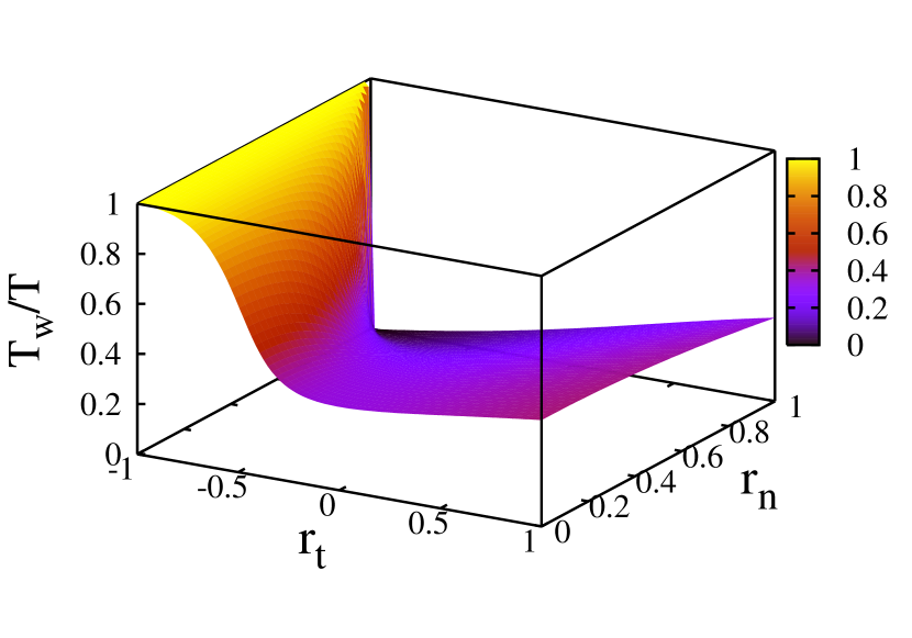
Figure 8: The ratio of average rotational energy to total energy as a function of the coefficients of normal, $r_{n}$, and tangential, $r_{t}$, restitution.

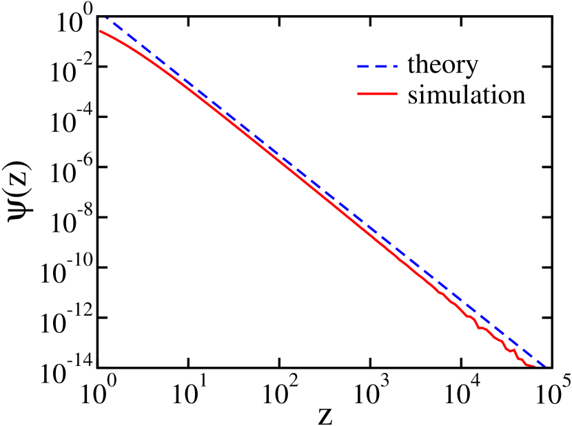
Figure 9: The scaling function underlying the energy distribution (solid line). The distribution was obtained using a Monte Carlo simulation with $N=10^{7}$ particles. A dashed line with the slope predicted by the theory is also shown for reference.

We solve this eigenvalue equation by performing a Monte Carlo simulation of the same angular process as described by (26) but with a different annihilation rate $\beta_{0}=1-\lambda(\nu-1)$. We compare the angle distribution predicted by (43) with the behavior of the energetic particles in the freely cooling gas.

The numerical simulations of the inelastic collision process confirm the theoretical predictions. First, the energy distribution is self-similar as in (40) and the characteristic scale is proportional to the temperature. Second, the distribution of the total energy has a power-law tail, as displayed in Fig. 9 and the exponent $\nu$ is very close to the theoretical prediction (numerical simulations of the collision process gives $\nu=2.98\pm 0.05$ while the eigenvalue equation yields $\nu=2.92\pm 0.05$).

The angle distribution deviates even more strongly from the uniform distribution with a very pronounced peak (see Fig. 11) because the dynamics are purely collisional. The singularities are weaker although the one at $x_{1}$ given by (30) is clear. The agreement between the solution of the angular process and the Monte Carlo simulations is slightly worse than for driven systems because the statistics become prohibitive: now it is necessary to probe the most energetic out of roughly $10^{6}$ particles to obtain the asymptotic angle distribution! The sharper power-law decay is responsible for this three order of magnitude increase: the cumulative distribution of total energy decays according to $\int_{E}dE^{\prime}p(E^{\prime})\sim E^{-\mu}$ with $\mu=\nu-1$ about three times larger than before. Finally, the angle distribution of all particles deviates only slightly from a uniform distribution (see Fig. 11). We conclude that the behavior of the freely cooling gas is qualitatively similar to that found in driven steady-states.

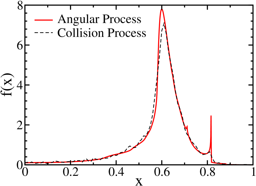
Figure 10: The angle distribution of the energetic particles. Shown are results for the collision process (solid line) and for the angular process (dashed line).

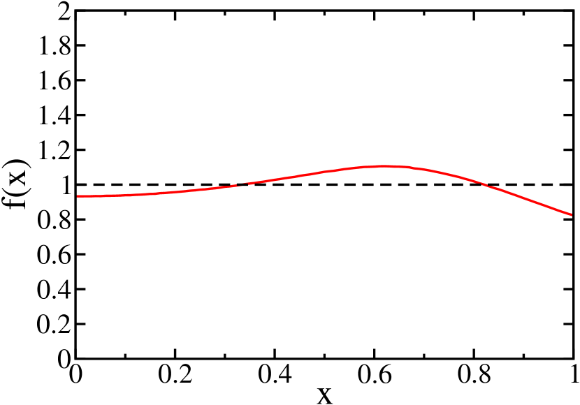
Figure 11: The angle distribution of all particles for a freely cooling gas (solid line). Also shown for reference is the uniform equilibrium distribution.

VI Conclusions and Outlook

The complete description of granular media with translational and rotational degrees of freedom requires the full bivariate distribution of energies. It is not sufficient to consider only the average kinetic energy of translations and rotations. Instead the full bivariate distribution is highly nontrivial. We have shown that in the limit of large particle energy, this distribution obeys a linear equation. Its solution can be written as a product of two distributions, one for the total energy, $E=E_{v}+E_{w}$, and one for the variable $x=\sqrt{E_{w}/E}$, which captures the partition of the total energy between rotational and translational motion. The distribution of the total energy decays algebraically and the characteristic exponent depends on the collision parameters and the moment of inertia. The variable $x$ is not uniformly distributed as in equilibrium. Instead the distribution $f(x)$ is not analytic and displays a series of singularities of varying strengths. Remarkably, there are special preferred ratios of rotational-to-total energy. This violation of energy equipartition among different degrees of freedom is a direct consequence of the energy dissipation. The total energy and the variable $x$ are correlated in general with the deviations from equilibrium increasing with energy. These two variable become uncorrelated only at extremely high-energies.

We have studied both, the system which is driven at extremely high energies and displays a stationary energy cascade on energy scales below the driving one, and a freely cooling gas. In the latter gas the bivariate energy distribution is time dependent, reflecting the overall decrease of energy. Nevertheless, scaling the total energy with temperature, one finds a self-similar form for the distribution, which again factorizes in the high-energy limit. As in the driven system, the distribution of the total energy decays as a power law with, however, different exponents for the driven and the free cooling system. The angular distribution deviates even more from the uniform (equipartition) one in the cooling system.

It should be straightforward to extend these results to three dimensions where the angular process takes place in three dimensions. In the limit of high energies one would again expect a limiting distribution for the partition angle $x=\sqrt{E_{w}/E}$. Another possible extension refers to a more realistic law of friction, including Coulomb friction Walton ; flca . Finally, it would be of interest to extend the analysis to other systems, where equipartition is violated. An example is a binary mixture, where the energy is shared unequally between the two components.

Appendix A The Collision rules

The total linear momentum ${\bf v}^{\prime}_{a}+{\bf v}^{\prime}_{b}={\bf v}_{a}+{\bf v}_{b}$ is conserved in the collision. The angular momenta of the two particles with respect to the point of contact, ${\bm{\omega}}^{\prime}_{i}$, are given by

$$I{\bm{\omega}}_{a} =I{\bf w}_{a}+m\,R\,\hat{\bf n}\times{\bf v}_{a}$$ (44a)

$$I{\bm{\omega}}_{b} =I{\bf w}_{b}-m\,R\,\hat{\bf n}\times{\bf v}_{b}.$$ (44b)

These are conserved, ${\bm{\omega}}^{\prime}_{i}={\bm{\omega}}_{i}$ with $i=a,b$, because there is no torque at the point of contact. In inelastic collisions, the normal and tangential components of the relative velocity at the point of contact obey the collision law (4) where ${\bf U}={\bf V}+R\,\hat{\bf n}\times{\bf W}$.

It is convenient to introduce the momentum transfer ${\bm{\delta}}$, defined as follows: ${\bf v}^{\prime}_{a}={\bf v}_{a}-{\bm{\delta}}$ and ${\bf v}^{\prime}_{b}={\bf v}_{b}+{\bm{\delta}}$. Conservation of the angular velocity with respect to the point of contact and Eq. (44) gives ${\bf w}^{\prime}_{i}={\bf w}_{i}+\frac{1}{qR}\,\hat{\bf n}\times{\bm{\delta}}$. In terms of ${\bm{\delta}}$, the difference in velocity at the point of contact is ${\bf U}^{\prime}={\bf U}-2{\bm{\delta}}+\frac{2}{q}\,\hat{\bf n}\times\hat{\bf n}\times{\bm{\delta}}$. Substituting this expression into the collision laws (4), the normal and the tangential components of ${\bm{\delta}}$ are simply

$${\bm{\delta}}\cdot\hat{\bf n} =\eta_{n}\,{\bf U}\cdot\hat{\bf n}$$ (45a)

$${\bm{\delta}}\times\hat{\bf n} =\eta_{t}\,{\bf U}\times\hat{\bf n}.$$ (45b)

Consequently, the momentum transfer is ${\bm{\delta}}=\eta_{n}{\bf U}\cdot\hat{\bf n}\,\hat{\bf n}+\eta_{t}({\bf U}-{\bf U}\cdot\hat{\bf n}\,\hat{\bf n})$ or explicitly,

$${\bm{\delta}}=\eta_{n}\,{\bf V}\cdot\hat{\bf n}\,\hat{\bf n}+\eta_{t}\left({\bf V}-{\bf V}\cdot\hat{\bf n}\,\hat{\bf n}\right)+\eta_{t}\,R\,\hat{\bf n}\times{\bm{W}}$$ (46)

We now have the explicit collision rules (5).

Appendix B Particle Number Conservation

In this appendix, we verify that the stationary solution is consistent with particle number conservation. Maxwell Molecules are considered for simplicity. It is straightforward to generalize this calculation to all $\gamma$ and to free cooling.

Our starting point is Eq. (21), specialized to Maxwell molecules, i.e. $\gamma=0$,

$$\frac{\partial P(E,\Omega)}{\partial t}\!=\!\int d\Omega_{0}\left[\frac{1}{\alpha_{1}}\!P\left(\!\frac{E}{\alpha_{1}},\Omega_{0}\!\right)\delta(\Omega-\Omega_{1})+\frac{1}{\alpha_{2}}\!P\left(\!\frac{E}{\alpha_{2}},\Omega_{0}\!\right)\delta(\Omega-\Omega_{2})-P(E,\Omega_{0})\delta(\Omega-\Omega_{0})\right].$$ (47)

As a first step we integrate this equation over the solid angle

$$\frac{\partial p(E)}{\partial t}\!=\!\int d\Omega_{0}\left[\frac{1}{\alpha_{1}}\!P\left(\!\frac{E}{\alpha_{1}},\Omega_{0}\!\right)+\frac{1}{\alpha_{2}}\!P\left(\!\frac{E}{\alpha_{2}},\Omega_{0}\!\right)-P(E,\Omega_{0})\right].$$ (48)

The power-law behavior (24) typically holds in a restricted energy range, $E_{l}\leq E\leq E_{u}$, where $E_{l}$ and $E_{u}$ are upper and lower cutoffs. In the driven case, the upper cutoff is set by the energy injection scale. Let $N=\int_{E_{l}}^{E_{u}}dE\,p(E)$ be the total number of particles in this range. With the powerlaw decay (24), then

$$N\sim\frac{1}{\nu-1}\left(E_{l}^{1-\nu}-E_{u}^{1-\nu}\right).$$ (49)

To evaluate this time evolution of $N$, we substitute the product form (23) into (48) and integrate over the energies in the aforementioned power-law range,

$$\frac{\partial N}{\partial t}=N\int d\Omega_{0}\,g(\Omega_{0})\left[\alpha_{1}^{\nu-1}+\alpha_{2}^{\nu-1}-1\right].$$ (50)

Using Eq. (27), we confirm that the total number of particles is conserved, $\partial N/\partial t=0$.

Appendix C The matrix coefficients

In an inelastic collision, the translational energy loss is $\Delta E_{v}=E_{v}-E_{v}^{\prime}$ with $E_{v}=\frac{1}{2}(v_{a}^{2}+v_{b}^{2})$ and similarly, the rotational energy loss is $\Delta E_{w}=E_{w}-E_{w}^{\prime}$ with $E_{w}=\frac{1}{2}q(w_{a}^{2}+w_{b}^{2})$. We can conveniently calculate these quantities by using ${\bf v}^{\prime}_{a}={\bf v}_{a}-{\bm{\delta}}$, ${\bf v}^{\prime}_{b}={\bf v}_{b}+{\bm{\delta}}$, and ${\bf w}^{\prime}_{i}={\bf w}_{i}+(1/qR)\hat{\bf n}\times{\bm{\delta}}$, and by expressing the momentum transfer ${\bm{\delta}}$ using the natural coordinate system, ${\bm{\delta}}=\eta_{n}\,V_{n}\hat{\bf n}+\eta_{t}(V_{t}-W)\hat{\bf t}$,

$$\Delta E_{v} =\eta_{n}(1-\eta_{n})V_{n}^{2}+\eta_{t}(1-\eta_{t})V_{t}^{2}-\eta_{t}^{2}W^{2}+\eta_{t}(2\eta_{t}-1)V_{t}W$$ (51a)

$$\Delta E_{w} =-(\eta_{t}^{2}/q)V_{t}^{2}+\eta_{t}(1-\eta_{t}/q)W^{2}-\eta_{t}(1-2\eta_{t}/q)V_{t}W.$$ (51b)

The rate of change of the respective temperatures equals $1/2$ the average of this quantities, $\frac{d}{dt}T_{v}=\frac{1}{2}\langle\Delta E_{v}\rangle$ and $\frac{d}{dt}T_{w}=\frac{1}{2}\langle\Delta E_{w}\rangle$. This is seen by multiplying (V) by $\frac{1}{2}v^{2}$ and by integrating over the velocity. The averaging is with respect to the probability distribution functions of the two colliding particles. The cross-term vanishes, $\langle V_{t}W\rangle=0$, by symmetry. Using $\langle V_{n}^{2}\rangle=2\langle v_{n}^{2}\rangle=\langle v^{2}\rangle=2T_{v}$ and $\langle W^{2}\rangle=2\langle w^{2}\rangle=4T_{w}/q$ we obtain the matrix elements (35).