Cosmological Shock Waves in the Large Scale Structure of the Universe: Non-gravitational Effects

Abstract

Cosmological shock waves result from supersonic flow motions induced by hierarchical clustering of nonlinear structures in the universe. These shocks govern the nature of cosmic plasma through thermalization of gas and acceleration of nonthermal, cosmic-ray (CR) particles. We study the statistics and energetics of shocks formed in cosmological simulations of a concordance $\Lambda$CDM universe, with a special emphasis on the effects of non-gravitational processes such as radiative cooling, photoionization/heating, and galactic superwind feedbacks. Adopting an improved model for gas thermalization and CR acceleration efficiencies based on nonlinear diffusive shock acceleration calculations, we then estimate the gas thermal energy and the CR energy dissipated at shocks through the history of the universe. Since shocks can serve as sites for generation of vorticity, we also examine the vorticity that should have been generated mostly at curved shocks in cosmological simulations. We find that the dynamics and energetics of shocks are governed primarily by the gravity of matter, so other non-gravitational processes do not affect significantly the global energy dissipation and vorticity generation at cosmological shocks. Our results reinforce scenarios in which the intracluster medium and warm-hot intergalactic medium contain energetically significant populations of nonthermal particles and turbulent flow motions.

1 Introduction

Astrophysical plasmas consist of both thermal particles and nonthermal, cosmic-ray (CR) particles that are closely coupled with permeating magnetic fields and underlying turbulent flows. In the interstellar medium (ISM) of our Galaxy, for example, an approximate energy equipartition among different components seems to have been established, i.e., $\varepsilon_{therm}\sim\varepsilon_{CR}\sim\varepsilon_{B}\sim\varepsilon_{turb}\sim 1\ {\rm eV\ cm^{-3}}$ (Longair, 1994). Understanding the complex network of physical interactions among these components constitutes one of fundamental problems in astrophysics.

There is substantial observational evidence for the presence of nonthermal particles and magnetic fields in the large scale structure of the universe. A fair fraction of X-ray clusters have been observed in diffuse radio synchrotron emission, indicating the presence of GeV CR electrons and $\mu$G fields in the intracluster medium (ICM) (Giovannini & Feretti, 2000). Observations in EUV and hard X-ray have shown that some clusters possess excess radiation compared to what is expected from the hot, thermal X-ray emitting ICM, most likely produced by the inverse-Compton scattering of cosmic background radiation (CBR) photons by CR electrons (Fusco-Femiano et al., 1999; Bowyer et al., 1999; Berghöfer et al., 2000). Assuming energy equipartition between CR electrons and magnetic fields, $\varepsilon_{CRe}\sim\varepsilon_{B}\sim 0.01-0.1{\rm eV\ cm^{-3}}\sim 10^{-3}-10^{-2}\varepsilon_{therm}$ can be inferred in typical radio halos (Govoni & Feretti, 2004). If some of those CR electrons have been energized at shocks and/or by turbulence, the same process should have produced a greater CR proton population. Considering the ratio of proton to electron numbers, $K\sim 100$, for Galactic CRs (Beck & Kraus, 2005), one can expect $\varepsilon_{CRp}\sim 0.01-0.1\varepsilon_{therm}$ in radio halos. However, CR protons in the ICM have yet to be confirmed by the observation of $\gamma$-ray photons produced by inelastic collisions between CR protons and thermal protons (Reimer et al., 2003). Magnetic fields have been also directly observed with Faraday rotation measure (RM). In clusters of galaxies strong fields of a few $\mu$G strength extending from core to 500 kpc or further were inferred from RM observations (Clarke et al., 2001; Clarke, 2004). An upper limit of $\lesssim\mu$G was imposed on the magnetic field strength in filaments and sheets, based the observed limit of the RMs of quasars outside clusters (Kronberg, 1994; Ryu et al., 1998).

Studies on turbulence and turbulent magnetic fields in the large scale structure of the universe have been recently launched too. XMM-Newton X-ray observations of the Coma cluster, which seems to be in a post-merger stage, were analyzed in details to extract clues on turbulence in the ICM (Schuecker et al., 2004). By analyzing pressure fluctuations, it was shown that the turbulence is likely subsonic and consistent with Kolmogoroff turbulence. RM maps of clusters have been analyzed to find the power spectrum of turbulent magnetic fields in a few clusters (Murgia et al., 2004; Vogt & Enßlin, 2005). While Murgia et al. (2004) reported a spectrum shallower than the Kolmogoroff spectrum, Vogt & Enßlin (2005) argued that the spectrum could be consistent with the Kolmogoroff spectrum if it is bended at a few kpc scale. These studies suggest that as in the ISM, turbulence does exist in the ICM and may constitute an energetically non-negligible component.

In galaxy cluster environments there are several possible sources of CRs, magnetic fields, and turbulence: jets from active galaxies (Kronberg et al., 2004; Li et al., 2006), termination shocks of galactic winds driven by supernova explosions (Vök & Atoyan, 1999), merger shocks (Sarazin, 1999; Gabici & Blasi, 2003; Fujita et al., 2003), structure formation shocks (Loeb & Waxmann, 2000; Miniati et al., 2001a, b), and motions of subcluster clumps and galaxies (Subramanian et al., 2006). All of them have a potential to inject a similar amount of energies, i.e., $E\sim 10^{61}-10^{62}$ ergs into the ICM. Here we focus on shock scenarios.

Astrophysical shocks are collisionless shocks that form in tenuous cosmic plasmas via collective electromagnetic interactions between gas particles and magnetic fields. They play key roles in governing the nature of cosmic plasmas: i.e., 1) shocks convert a part of the kinetic energy of bulk flow motions into thermal energy, 2) shocks accelerate CRs by diffusive shock acceleration (DSA) (Blandford & Ostriker, 1978; Blandford & Eichler, 1987; Malkov & Drury, 2001), and amplify magnetic fields by streaming CRs (Bell, 1978; Lucek & Bell, 2000), 3) shocks generate magnetic fields via the Biermann battery mechanism (Biermann, 1950; Kulsrud et al., 1997) and the Weibel instability (Weibel, 1959; Medvedev et al., 2006), and 4) curved shocks generate vorticity and ensuing turbulent flows (Binney, 1974; Davies & Widrow, 2000).

In Ryu et al. (2003) (Paper I), the properties of cosmological shock waves in the intergalactic medium (IGM) and the energy dissipations into thermal and nonthermal components at those shocks were studied in a high-resolution, adiabatic (non-radiative), hydrodynamic simulation of a $\Lambda$CDM universe. They found that internal shocks with low Mach numbers of $M\lesssim 4$, which formed in the hot, previously shocked gas inside nonlinear structures, are responsible for most of the shock energy dissipation. Adopting a nonlinear DSA model for CR protons, it was shown that about $1/2$ of the gas thermal energy dissipated at cosmological shocks through the history of the universe could be stored as CRs. In a recent study, Pfrommer et al. (2006) identified shocks and analyzed the statistics in smoothed particle hydrodynamic (SPH) simulations of a $\Lambda$CDM universe, and found that their results are in good agreement with those of Paper I. While internal shocks with lower Mach numbers are energetically dominant, external accretions shocks with higher Mach numbers can serve as possible acceleration sites for high energy cosmic rays (Kang et al., 1996, 1997; Ostrowski & Siemieniec-Ozieblo, 2002). It was shown that CR ions could be accelerated up to $\sim Z\times 10^{19}eV$ at cosmological shocks, where $Z$ is the charge of ions (Inoue et al., 2007).

Ryu et al. (2007) (Paper II) analyzed the distribution of vorticity, which should have been generated mostly at cosmological shock waves, in the same simulation of a $\Lambda$CDM universe as in Paper I, and studied its implication on turbulence and turbulence dynamo. Inside nonlinear structures, vorticity was found to be large enough that the turn-over time, which is defined as the inverse of vorticity, is shorter than the age of the universe. Based on it Ryu et al. (2007) argued that turbulence should have been developed in those structures and estimated the strength of the magnetic field grown by the turbulence.

In this paper, we study cosmological shock waves in a new set of hydrodynamic simulations of large structure formation in a concordance $\Lambda$CDM universe: an adiabatic (non-radiative) simulation which is similar to that considered in Paper I, and two additional simulations which include various non-gravitational processes (see the next section for details). As in Papers I and II, the properties of cosmological shock waves are analyzed, the energy dissipations to gas thermal energy and CR energy are evaluated, and the vorticity distribution is analyzed. We then compare the results for the three simulations to highlight the effects of non-gravitational processes on the properties of shocks and their roles on the cosmic plasmas in the large scale structure of the universe.

Simulations are described in §2. The main results of shock identification and properties, energy dissipations, and vorticity distribution are described in §3, §4, and §5, respectively. Summary and discussion are followed in §6.

2 Simulations

The results reported here are based on the simulations previously presented in Cen & Ostriker (2006). The simulations included radiative processes of heating/cooling, and the two simulations with and without galactic superwind (GSW) feedbacks were compared in that paper. Here an additional adiabatic (non-radiative) simulation with otherwise the same setup was performed. Hereafter these three simulations are referred as “Adiabatic”, “NO GSW”, and “GSW” simulations, respectively. Specifically, the WMAP1-normalized $\Lambda$CDM cosmology was employed with the following parameters: $\Omega_{b}=0.048$, $\Omega_{m}=0.31$, $\Omega_{\Lambda}=0.69$, $h\equiv H_{0}$/(100 km/s/Mpc) = 0.69, $\sigma_{8}=0.89$, and $n=0.97$. A cubic box of comoving size $85~{}h^{-1}{\rm Mpc}$ was simulated using $1024^{3}$ grid zones for gas and gravity and $512^{3}$ particles for dark matter. It allows a uniform spatial resolution of $\Delta l=83~{}h^{-1}{\rm kpc}$. In Papers I and II, an adiabatic simulation in a cubic box of comoving size $100~{}h^{-1}{\rm Mpc}$ with $1024^{3}$ grid zones and $512^{3}$ particles, employing slightly different cosmological parameters, was used. The simulations were performed using a PM/Eulerian hydrodynamic cosmology code (Ryu et al., 1993).

Detailed descriptions for input physical ingredients such as non-equilibrium ionization/cooling, photoionization/heating, star formation, and feedback processes can be found in earlier papers (Cen et al., 2003; Cen & Ostriker, 2006). Feedbacks from star formation were treated in three forms: ionizing UV photons, GSWs, and metal enrichment. GSWs were meant to represent cumulative supernova explosions, and modeled as outflows of several hundred $~{}{\rm km~{}s^{-1}}$. The input of GSW energy for a given amount of star formation was determined by matching the outflow velocities computed for star-burst galaxies in the simulation with those observed in the real world (Pettini et al., 2002)(see also Cen & Ostriker, 2006, for details).

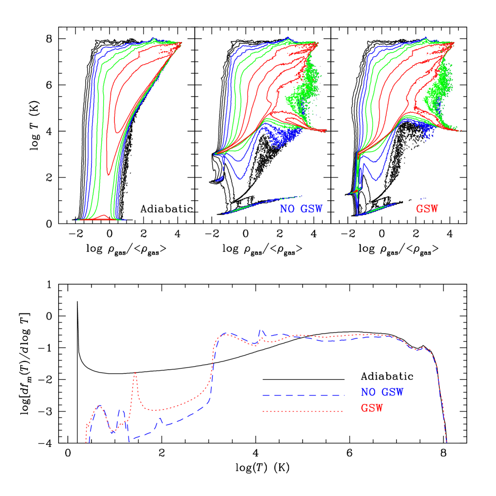
Figure 1: Top panels: Gas mass distribution in the gas density-temperature plane at $z=0$ for the Adiabatic, NO GSW, and GSW simulations. Bottom panel: Gas mass fraction as a function of gas temperature at $z=0$ for the three simulations.

Figure 1 shows the gas mass distribution in the gas density-temperature plane, $f_{m}(\rho_{gas},T)$, and the gas mass fraction as a function of gas temperature, $f_{m}(T)$, at $z=0$ for the three simulations. The distributions are quite different, depending primarily on the inclusion of radiative cooling and photoionization/heating. GSW feedbacks increase the fraction of the WHIM with $10^{5}<T<10^{7}$K, and at the same time affect the distribution of the warm/diffuse gas with $T<10^{5}$.

3 Properties of Cosmological Shock Waves

We start to describe cosmological shocks by briefing the procedure by which the shocks were identified in simulation data. The details can be found in Paper I. A zone was tagged as a shock zone currently experiencing shock dissipation, whenever the following three criteria are met: 1) the gradients of gas temperature and entropy have the same sign, 2) the local flow is converging with ${\vec{\nabla}}\cdot{\vec{v}}<0$, and 3) $|\Delta\log T|\geq 0.11$ corresponding to the temperature jump of a shock with $M\geq 1.3$. Typically a shock is represented by a jump spread over $2-3$ tagged zones. Hence, a shock center was identified within the tagged zones, where ${\vec{\nabla}}\cdot{\vec{v}}$ is minimum, and this center was labeled as part of a shock surface. The Mach number of the shock center, $M$, was calculated from the temperature jump across the entire shock zones. Finally to avoid confusion from complex flow patterns and shock surface topologies associated with very weak shocks, only those portions of shock surfaces with $M\geq 1.5$ were kept and used for the analysis of shocks properties.

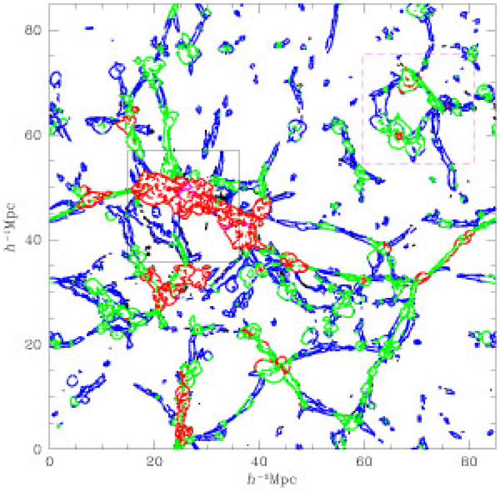
Figure 2: Two-dimensional slice of $(85~{}h^{-1}{\rm Mpc})^{2}$ showing shock locations at $z=0$ in the GSW simulation, which are color-coded according to shock speed as follows: black for $V_{s}<15~{}{\rm km~{}s^{-1}}$, blue for $15\leq V_{s}<65~{}{\rm km~{}s^{-1}}$, green for $65\leq V_{s}<250~{}{\rm km~{}s^{-1}}$, red for $250\leq V_{s}<1000~{}{\rm km~{}s^{-1}}$, and magenta for $V_{s}\geq 1000~{}{\rm km~{}s^{-1}}$. A blown-up image of the box (dashed line) in the upper right corner is shown in Figure 3, while a blown-up image of the box (solid line) around two merging clusters is shown in Figure 7.

Figure 2 shows the locations of identified shocks in a two-dimensional slice at $z=0$ in the GSW simulation. The locations are color-coded according to shock speed. As shown before in Paper I, external accretion shocks encompass nonlinear structures and reveal, in addition to cluster complexes, rich topology of filamentary and sheet-like structures in the large scale structure. Inside the nonlinear structures, there exist complex networks of internal shocks that form by infall of previously shocked gas to filaments and knots and during subclump mergers, as well as by chaotic flow motions. The shock heated gas around clusters extends out to $\sim 5~{}h^{-1}{\rm Mpc}$, much further out than the observed X-ray emitting volume.

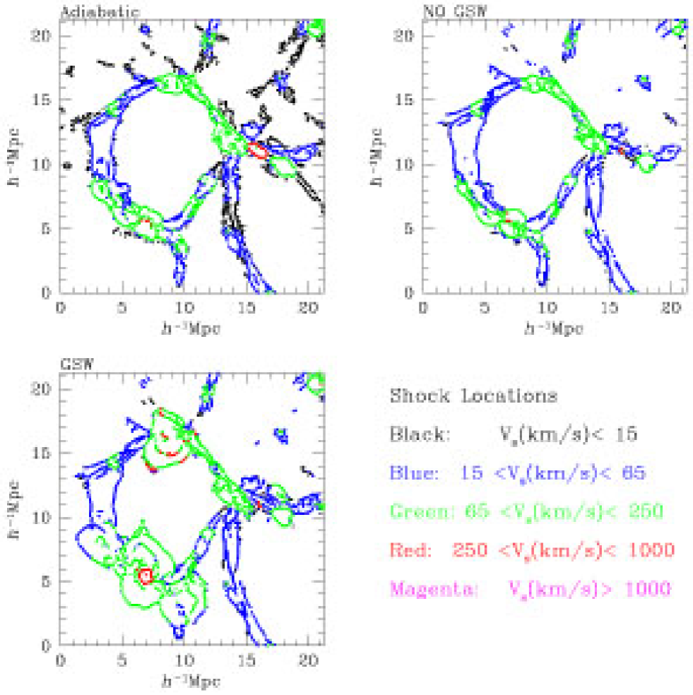
Figure 3: Two-dimensional slice of $(21.25~{}h^{-1}{\rm Mpc})^{2}$ showing shock locations at $z=0$ in the Adiabatic, NO GSW and GSW simulations. The locations are color-coded according to shock speed. Two groups in the GSW simulation have $kT\sim 0.2-0.3$ keV.

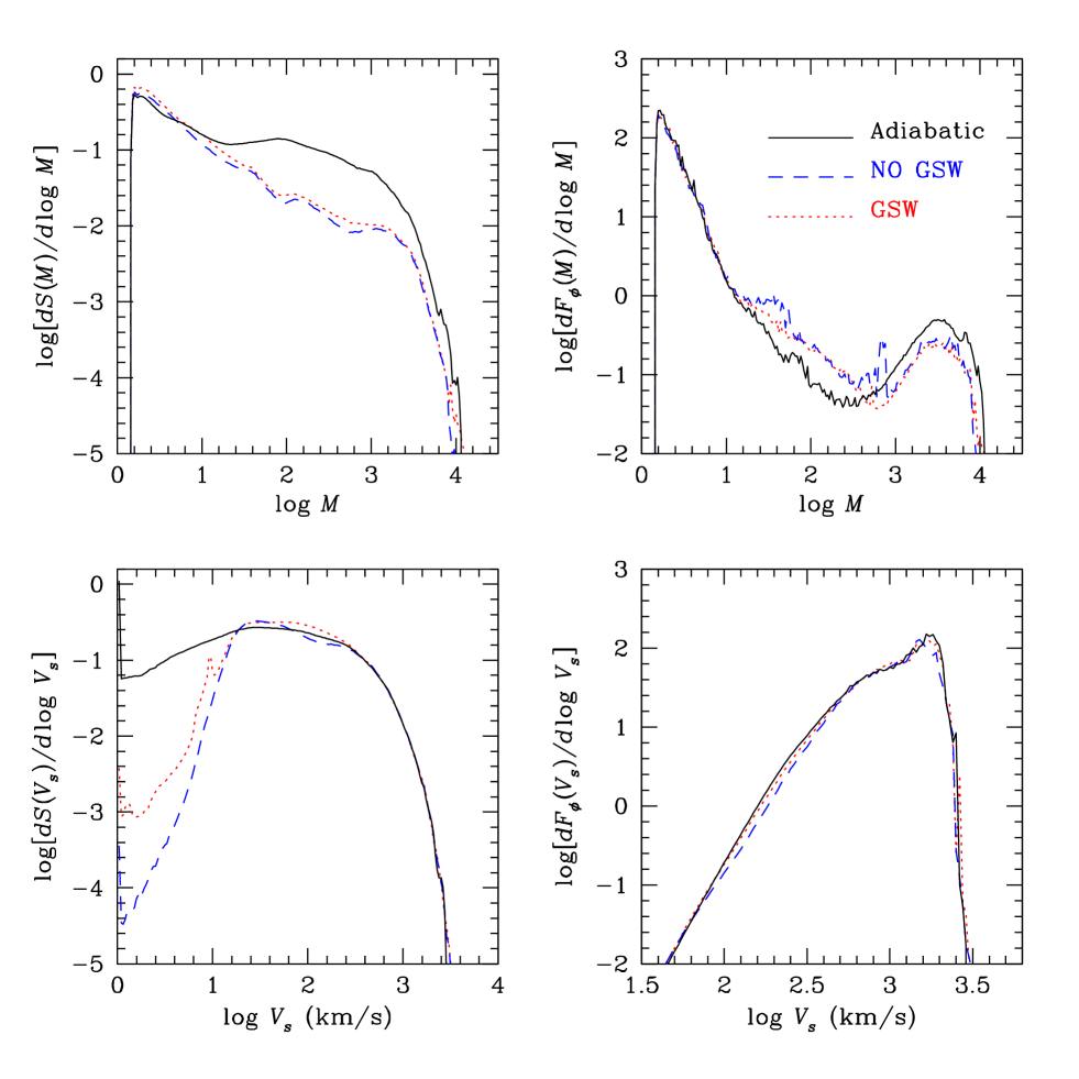
Figure 4: Left panels: Inverse of the mean comoving distance between shock surfaces as a function of Mach number $M$ (top) and shock speed $V_{s}$ (bottom) at $z=0$ for the Adiabatic (solid line), NO GSW (dashed line), and GSW (dotted line) simulations. Right panels: Kinetic energy flux per comoving volume passing through shock surfaces in units of $10^{40}$ ergs s^-1 $(h^{-1}{\rm Mpc})^{-3}$ as a function of $M$ (top) and $V_{s}$ (bottom). Note that the bottom two panels have different ranges of abscissa.

In the GSW simulation, with several hundred $~{}{\rm km~{}s^{-1}}$ for outflows, the GSW feedbacks affected most greatly the gas around groups of galaxies, while the impact on clusters with $kT\gtrsim 1$ keV was minimal. In Figure 3 we compare shock locations in a region around two groups with $kT\sim 0.2-0.3$ keV in the three simulations. It demonstrates that GSW feedbacks pushed the hot gas out of groups with typical velocities of $\sim 100~{}{\rm km~{}s^{-1}}$ (green points). In fact the prominent green balloons of shock surfaces around groups in Figure 2 are due to GSW feedbacks (see also Figure 4 of Cen & Ostriker, 2006).

In the left panels of Figure 4 we compare the surface area of identified shocks, normalized by the volume of the simulation box, per logarithmic Mach number interval, $dS(M)/d\log M$ (top), and per logarithmic shock speed interval, $dS(V_{s})/d\log V_{s}$ (bottom), at $z=0$ in the three simulations. Here $S$ and $V_{s}$ are given in units of $(h^{-1}{\rm Mpc})^{-1}$ and $~{}{\rm km~{}s^{-1}}$. The quantity $S$ provides a measure of shock frequency or the inverse of the mean comoving distance between shock surfaces. The distributions of $dS(M)/d\log M$ for the NO GSW and GSW simulations are similar, while that for the Adiabatic simulation is different from the other two. This is mainly because the gas temperature outside nonlinear structures is lower without photoionization/heating in the Adiabatic simulation. As a result, external accretion shocks tend to have higher Mach number due to colder preshock gas. The distribution of $dS(V_{s})/d\log V_{s}$, on the other hand, is similar for all three simulations for $V_{s}>15~{}{\rm km~{}s^{-1}}$. For $V_{s}<15~{}{\rm km~{}s^{-1}}$, however, there are more shocks in the Adiabatic simulation (black points in Figure 3). Again this is because in the Adiabatic simulation the gas temperature is colder in void regions, and so even shocks with low speeds of $V_{s}<15~{}{\rm km~{}s^{-1}}$ were identified in these regions. The GSW simulation shows slightly more shocks than the NO GSW simulation around $V_{s}\sim 100~{}{\rm km~{}s^{-1}}$, because GSW feedbacks created balloon-shaped surfaces of shocks with typically those speeds (green points in Figure 3).

For identified shocks, we calculated the incident shock kinetic energy flux, $F_{\phi}=(1/2)\rho_{1}V_{s}^{3}$, where $\rho_{1}$ is the preshock gas density. We then calculated the kinetic energy flux through shock surfaces, normalized by the volume of the simulation box, per logarithmic Mach number interval, $dF_{\phi}(M)/d\log M$, and per logarithmic shock speed interval, $dF_{\phi}(V_{s})/d\log V_{s}$. In the right panels of Figure 4, we compare the flux at $z=0$ in the three simulations. Once again, there are noticeable differences in $dF_{\phi}(M)/d\log M$ between the Adiabatic simulation and the other two simulations, which can be interpreted as the result of ignoring photoionization/heating in the gas outside nonlinear structures in the Adiabatic simulation. GSW feedbacks enhance only slightly the shock kinetic energy flux for $V_{s}\sim 100-300~{}{\rm km~{}s^{-1}}$, as can be seen in the plot of $dF_{\phi}(V_{s})/d\log V_{s}$. Yet, the total amount of the energy flux is expected to be quite similar for all three simulations. This implies that the overall energy dissipation at cosmological shocks is governed mainly by the gravity of matter, and that the inclusion of various non-gravitational processes such as radiative cooling, photoionization/heating, and GSW feedbacks have rather minor, local effects.

We note that a temperature floor of $T_{\rm floor}=T_{\rm CBR}$ was used for the three simulations in this work, while $T_{\rm floor}=10^{4}$ K was set in paper I. It was because in Paper I only an adiabatic simulation was considered and the $10^{4}$ K temperature floor was enforced to mimic the effect of photoionization/heating on the IGM. However we found that when the same temperature floor is enforced, the statistics of the current Adiabatic simulation agree excellently with those of Paper I. Specifically, the shock frequency and kinetic energy flux, $dS(M)/d\log M$ and $dF_{\phi}(M)/d\log M$, for weak shocks with $1.5\leq M\lesssim 3$ are a bit higher in the current Adiabatic simulation, because of higher spatial resolution. But the total kinetic energy flux through shock surfaces, $F_{\phi}(M>1.5)$, agrees within a few percent. On the other hand, In Paper I we were able to reasonably distinguish external and internal shocks according to the preshock temperature, i.e., external shocks if $T_{1}\leq T_{\rm floor}$ and internal shocks if $T_{1}>T_{\rm floor}$. We no longer made such distinction in this work, since the preshock temperature alone cannot tell us whether the preshock gas is inside nonlinear structures or not in the simulations with radiative cooling.

4 Energy dissipation by Cosmological Shock Waves

The CR injection and acceleration rates at shocks depend in general upon the shock Mach number, field obliquity angle, and the strength of the Alfvén turbulence responsible for scattering. At quasi-parallel shocks, in which the mean magnetic field is parallel to the shock normal direction, small anisotropy in the particle velocity distribution in the local fluid frame causes some particles in the high energy tail of the Maxwellian distribution to stream upstream (Giacalone et al., 1992). The streaming motions of the high energy particles against the background fluid generate strong MHD Alfvén waves upstream of the shock, which in turn scatter particles and amplify magnetic fields (Bell, 1978; Lucek & Bell, 2000). The scattered particles can then be accelerated further to higher energies via Fermi first order process (Malkov & Drury, 2001). These processes, i.e., leakage of suprathermal particles into CRs, self-excitation of Alfvén waves, amplification of magnetic fields, and further acceleration of CRs, are all integral parts of collisionless shock formation in astrophysical plasmas. It was shown that at strong quasi-parallel shocks, $10^{-4}-10^{-3}$ of the incoming particles can be injected into the CR population, up to 60% of the shock kinetic energy can be transferred into CR ions, and at the same time substantial nonlinear feedbacks are exerted to the underlying flow (Berezhko et al., 1995; Kang & Jones, 2005).

At perpendicular shocks with weakly perturbed magnetic fields, on the other hand, particles gain energy mainly by drifting along the shock surface in the ${\vec{v}}\times{\vec{B}}$ electric field. Such drift acceleration can be much more efficient than the acceleration at parallel shocks (Jokipii, 1987; Kang et al., 1997; Ostrowski & Siemieniec-Ozieblo, 2002). But the particle injection into the acceleration process is expected to be inefficient at perpendicular shocks, since the transport of particles normal to the average field direction is suppressed (Ellison et al., 1995). However, Giacalone (2005) showed that the injection problem at perpendicular shocks can be alleviated substantially in the presence of fully turbulent fields owing to field line meandering.

As in Paper I, the gas thermalization and CR acceleration efficiencies are defined as $\delta(M)\equiv F_{th}/F_{\phi}$ and $\eta(M)\equiv F_{CR}/F_{\phi}$, respectively, where $F_{th}$ is the thermal energy flux generated and $F_{CR}$ is the CR energy flux accelerated at shocks. We note that for gasdynamical shocks without CRs, the gas thermalization efficiency can be calculated from the Rankine-Hugoniot jump condition, as follows:

$$\delta_{0}(M)=\left[e_{th,2}-e_{th,1}\left({\rho_{2}\over\rho_{1}}\right)^{\gamma}\right]v_{2}\Bigg{/}\left({1\over 2}\rho_{1}v_{1}^{2}\right),$$ (1)

where the subscripts 1 and 2 stand for preshock and postshock regions, respectively. The second term inside the brackets subtracts the effect of adiabatic compression occurred at a shock too, not just the thermal energy flux entering the shock, namely, $e_{th,1}v_{1}$.

At CR modified shocks, however, the gas thermalization efficiency can be much smaller than $\delta_{0}(M)$ for strong shocks with large $M$, since a significant fraction of the shock kinetic energy can be transferred to CRs. The gas thermalization and CR acceleration efficiencies were estimated using the results of DSA simulations of quasi-parallel shocks with Bohm diffusion coefficient, self-consistent treatments of thermal leakage injection, and Alfvén wave propagation (Kang & Jones, 2007). The simulations were started with purely gasdynamical shocks in one-dimensional, plane-parallel geometry, and CR acceleration was followed by solving the diffusion-convection equation explicitly with very high resolution. Shocks with $V_{s}=150-4500$ km s^-1 propagating into media of $T_{1}=10^{4}-10^{6}$ K were considered. After a quick initial adjustment, the postshock states reach time asymptotic values and the CR modified shocks evolve in an approximately self-similar way with the shock structure broadening linearly with time (refer Kang & Jones, 2007, for details). Given this self-similar nature of CR modified shocks, we calculated time asymptotic values of $\delta(M)$ and $\eta(M)$ as the ratios of increases in the gas thermal and CR energies at shocks to the kinetic energy passed through the shocks at the termination time of the DSA simulations. As in Eq. (1), the increase of energies due to adiabatic compression was subtracted.

Figure 5 shows $\delta(M)$ and $\eta(M)$ estimated from DSA simulations and their fittings for the cases with and without a preexisting CR component. The fitting formulae are given in Appendix A. Without a preexisting CR component, gas thermalization is more efficient than CR acceleration at shocks with $M\lesssim 5$. However, it is likely that weak internal shocks propagate through the IGM that contains CRs accelerated previously at earlier shocks. In that case, shocks with preexisting CRs need to be considered. Since the presence of preexisting CRs is equivalent to a higher injection rate, CR acceleration is more efficient in that case, especially at shocks with $M\lesssim 5$ (Kang & Jones, 2003). In the bottom panel the efficiencies for shocks with $P_{CR}/P_{g}\sim 0.3$ in the preshock region are shown. For comparison, $\delta_{0}(M)$ for shocks without CRs is also drawn. Both $\delta(M)$ and $\eta(M)$ increase with Mach number, but $\eta(M)$ asymptotes to $\sim 0.55$ while $\delta(M)$ to $\sim 0.30$ for strong shocks with $M\gtrsim 30$. So about twice more energy goes into CRs, compared to for gas heating, at strong shocks.

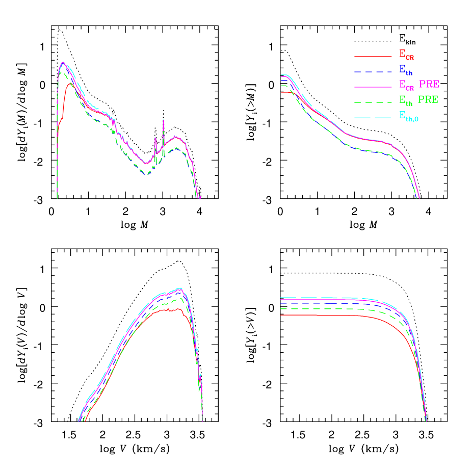
Figure 6: Left panels: Shock kinetic energy passed, $dY_{\phi}$ (dotted line), thermal energy dissipated, $dY_{th}$ (dashed line), and CR energy dissipated, $dY_{CR}$ (solid line), through surfaces of cosmological shocks with Mach number between $\log M$ and $\log M+d(\log M)$ (top) and through surfaces of cosmological shocks with shock speed between $\log V_{s}$ and $\log V_{s}+d(\log V_{s})$ (bottom), integrated from $z=5$ to $z=0$. Red and magenta lines are the CR energy for the cases without and with preexisting CRs, respectively. Blue and green lines are the thermal energy for the cases without and with preexisting CRs, respectively. The thermal energy expected to be dissipated at cosmological shocks without CRs (long dashed cyan line) is also plotted for comparison. Right panels: Cumulative energy distributions, $Y_{i}(>M)$ (top) and $Y_{i}(>V_{s})$ (bottom), for Mach number greater than $M$ and for shock speed greater than $V_{s}$. The energies are normalized by the gas thermal energy at $z=0$ inside the simulation box

The efficiencies for the case without a preexisting CR component in the upper panel of Figure 5 can be directly compared with the same quantities presented in Figure 6 of Paper I. In Paper I, however, the gas thermalization efficiency was not calculated explicitly from DSA simulations, and hence $\delta_{0}(M)$ for gasdynamic shocks was used. It represents gas thermalization reasonably well for weak shocks with $M\lesssim 2.5$, but overestimates gas thermalization for stronger CR modified shocks. Our new estimate for $\eta(M)$ is close to that in Paper I, but a bit smaller, especially for shocks with $M\lesssim 30$. This is because inclusion of Alfvén wave drift and dissipation in the shock precursor reduces the effective velocity change experienced by CRs in the new DSA simulations of Kang & Jones (2007).

A note of caution for $\eta(M)$ should be in order. As outlined above, CR injection is less efficient and so the CR acceleration efficiency would be lower at perpendicular shocks, compared to at quasi-parallel shocks. CR injection and acceleration at oblique shocks are not well understood quantitatively. And the magnetic field directions at cosmological shocks are not known. Considering these and other uncertainties involved in the adopted DSA model, we did not attempt to make further improvements in estimating $\delta(M)$ and $\eta(M)$ at general oblique shocks. But we expect that an estimate at realistic shocks with chaotic magnetic fields and random shock obliquity angles would give reduced values, rather than increased values, for $\eta(M)$. So $\eta(M)$ given in Figure 5 may be regarded as upper limits.

By adopting the efficiencies in Figures 5, we calculated the thermal and CR energy fluxes dissipated at cosmological shocks, $dF_{th}(M)/d\log M$, $dF_{th}(V_{s})/d\log V_{s}$, $dF_{CR}(M)/d\log M$ and $dF_{CR}(V_{s})/d\log V_{s}$, using $F_{th}=F_{\phi}\delta(M)$ and $F_{CR}=F_{\phi}\eta(M)$, in the same way we calculated $dF_{\phi}(M)/d\log M$ and $dF_{\phi}(V_{s})/d\log V_{s}$ in the previous section. We then integrated from $z=5$ to $z=0$ the shock kinetic energy passed and the thermal and CR energies dissipated through shock surfaces as follows:

$${{dY_{i}(X)}\over{d\log X}}={1\over{\cal E}_{th,0}}\int_{z=5}^{z=0}{{dF_{i}[X,z(t)]}\over{d\log X}}dt,$$ (2)

where the subscript $i\equiv\phi,~{}th,~{}{\rm or}~{}CR$ stands for the kinetic, thermal, or CR energies fluxes, the variable $X$ is either $M$ or $V_{s}$, and ${\cal E}_{th,0}$ is the total gas thermal energy at $z=0$ inside the simulation box normalized by its volume.

Figure 6 shows the resulting ${dY_{i}(M)}/{d\log M}$ and ${dY_{i}(V_{s})}/{d\log V_{s}}$ and their cumulative distributions, $Y_{i}(>M)$ and $Y_{i}(>V_{s})$, for the GSW simulation. Weak shocks with $M\lesssim 4$ or fast shocks with $V_{s}\gtrsim 500~{}{\rm km~{}s^{-1}}$ are responsible most for shock dissipations, as already noted in Paper I. While the thermal energy generation peaks at shocks in the range $1.5\lesssim M\lesssim 3$, the CR energy peaks in the range $2,5\lesssim M\lesssim 4$ if no preexisting CRs are included or in the range $1.5\lesssim M\lesssim 3$ if preexisting CRs of $P_{CR}/P_{g}\sim 0.3$ in the preshock region are included. With our adopted efficiencies, the total CR energy accelerated and the total gas thermal energy dissipated at cosmological shocks throughout the history of the universe are compared as $Y_{CR}(M\geq 1.5)\sim 0.5Y_{th}(M\geq 1.5)$, when no preexisting CRs are present. With preexisting CRs in the preshock region, the CR acceleration becomes more efficient, so $Y_{CR}(M\geq 1.5)\sim 1.7Y_{th}(M\geq 1.5)$, i.e., the total CR energy accelerated at cosmological shocks is estimated to be 1.7 times the total gas thermal energy dissipated. We note here again that these are not meant to be very accurate estimates of the CR energy in the IGM, considering the difficulty of modeling shocks as well as the uncertainties in the DSA model itself. However, they imply that the IGM and the WHIM, which are bounded by strong external shocks with high $M$ and filled with weak internal shocks with low $M$, could contain a dynamically significant CR population.

5 Vorticity Generation at Cosmological Shock Waves

Cosmological shocks formed in the large scale structure of the universe are by nature curved shocks, accompanying complex, often chaotic flow patterns. It is well known that vorticity, ${\vec{\omega}}=\nabla\times{\vec{v}}$, is generated at such curved oblique shocks (Binney, 1974; Davies & Widrow, 2000). In Paper II, the generation of vorticity behind cosmological shocks and turbulence dynamo of magnetic fields in the IGM were studied in an adiabatic $\Lambda$CDM simulation. In this study we analyzed the distribution of vorticity in the three simulations to assess quantitatively the effects of non-gravitational processes. Here we present the magnitude of vorticity with the vorticity parameter

$$\tau({\vec{r}},z)\equiv t_{\rm age}(z)\omega({\vec{r}},z)={t_{\rm age}(z)\over t_{\rm eddy}({\vec{r}},z)},$$ (3)

where $t_{\rm age}(z)$ is the age of the universe at redshift $z$. With $t_{\rm eddy}=1/\omega$ interpreted as local eddy turnover time, $\tau$ represents the number of local eddy turnovers in the age of the universe. So if $\tau\gg 1$, we expect that turbulence has been fully developed after many turnovers.

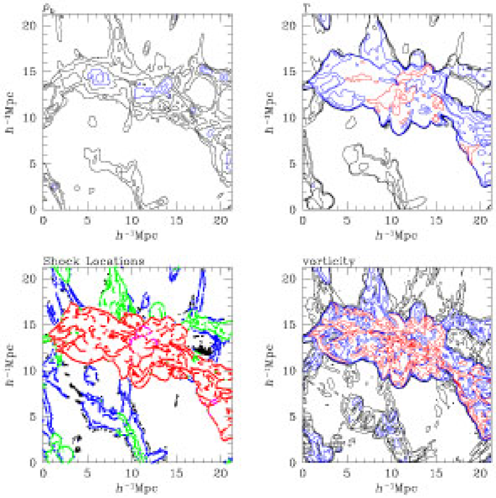
Figure 7: Two-dimensional slice of $(21.25~{}h^{-1}{\rm Mpc})^{2}$ around two merging clusters with $kT\sim 1-2$ keV at $z=0$ in the GSW simulation. Distributions of gas density (top left), temperature (top right), shock locations (bottom left), and vorticity (bottom right) are shown. In the gas density, temperature, and vorticity distributions, back, blue and red contours represent regions of low, middle, and high values, respectively.

Figure 7 shows fluid quantities and shock locations in a two-dimensional slice of $(21.25~{}h^{-1}{\rm Mpc})^{2}$, delineated by a solid box in Figure 2, at $z=0$ in the GSW simulations. The region contains two clusters with $kT\sim 1-2$ keV in the process of merging. Bottom right panel shows that vorticity increases sharply at shocks. The postshock gas has a larger amount of vorticity than the preshock gas, indicating that most, if not all, of the vorticity in the simulation was produced at shocks.

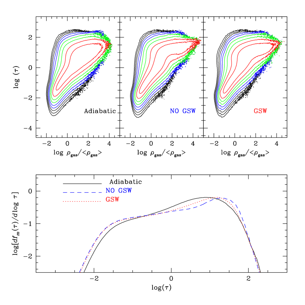
Figure 8: Top panels: Gas mass distribution in the gas mass density-vorticity parameter plane at $z=0$ for the Adiabatic, NO GSW, and GSW simulations. The vorticity parameter is defined as $\tau=\omega t_{age}(z)$, where $\omega=|{\vec{\nabla}}\times{\vec{v}}|$ and $t_{age}(z)$ is the age of the universe at redshift $z$. Bottom panel: Gas mass fraction as a function of vorticity parameter at $z=0$ for the three simulations.

Figure 8 shows the gas mass distribution in the gas density-vorticity parameter plane, $f_{m}(\rho_{gas},\tau)$, (upper panel) and the gas mass fraction per logarithmic $\tau$ interval, $df_{m}(\tau)/d\log\tau$, (bottom panel) for the three simulations. The most noticeable point in the upper panel is that vorticity is higher at the highest density regions with $\tilde{\rho}\equiv\rho_{gas}/\langle\rho_{gas}\rangle\gtrsim 10^{3}$ in the NO GSW and GSW simulations than in the Adiabatic simulation. This is due to the additional flow motions induced by cooling. Inclusion of GSW feedbacks, on the other hand, does not alter significantly the overall distribution in the gas density-vorticity parameter plane. The bottom panel indicates that cooling increased the mass fraction with large vorticity $\tau\gtrsim 10$, while reduced the mass fraction with $1\lesssim\tau\lesssim 10$. GSW feedbacks increased slightly the mass fraction with $1\lesssim\tau\lesssim 10$, which corresponds to the gas in the regions outskirts of groups that expand further out due to GSWs (i.e., balloons around groups). But overall we conclude that the non-gravitational processes considered in this paper have limited effects on vorticity in the large scale structure of the universe.

We note that the highest density regions in the NO GSW and GSW simulations have $\tau\sim 30$ on average. As described in details in Paper II, such values of $\tau$ imply that local eddies have turned over many times in the age of the universe, so that the ICM gas there has had enough time to develop magnetohydrodynamic (MHD) turbulence. So in those regions, magnetic fields should have grown to have the energy approaching to the turbulent energy. On the other hand, the gas with $1\lesssim\tilde{\rho}\lesssim 10^{3}$, mostly in filamentary and sheet-like structures, has $0.1\lesssim\tau\lesssim 10$. MHD turbulence should not have been fully developed there and turbulence growth of magnetic fields would be small. Finally in the low density void regions with $\tilde{\rho}\lesssim 1$, vorticity is negligible with $\tau\lesssim 0.1$ on average, as expected.

6 Summary

We identified cosmological shock waves and studied their roles on cosmic plasmas in three cosmological N-body/hydrodynamic simulations for a concordance $\Lambda$CDM universe in a cubic box of comoving size $85~{}h^{-1}{\rm Mpc}$: 1) adiabatic simulation (Adiabatic), 2) simulation with radiative cooling and photoionization/heating (NO GSW), and 3) same as the second simulation but also with galactic superwind feedbacks (GSW). The statistics and energetics of shocks in the adiabatic simulation are in an excellent agreement with those of Paper I where an adiabatic simulation with slightly different cosmological parameters in a cubic box of comoving size $100~{}h^{-1}{\rm Mpc}$ was analyzed.

Photoionization/heating raised the gas temperature outside nonlinear structures in the NO GSW and GSW simulations. As a result, the number of identified shocks and their Mach numbers in the NO GSW and GSW simulations were different from those in the Adiabatic simulation. GSW feedbacks pushed out gas most noticeably around groups, creating balloon-shaped surfaces of shocks with speed $V_{s}\sim 100~{}{\rm km~{}s^{-1}}$ in the GSW simulation. However, those have minor effects on shock energetics. The total kinetic energy passed through shock surfaces throughout the history of the universe is very similar for all three simulations. So we conclude that the energetics of cosmological shocks was governed mostly by the gravity of matter, and the effects non-gravitational processes, such as radiative cooling, photoionization/heating, and GSW feedbacks, were rather minor and local.

We estimated both the improved gas thermalization efficiency, $\delta(M)$, and CR acceleration efficiency, $\eta(M)$, as a function shock Mach number, from nonlinear diffusive shock simulations for quasi-parallel shocks that assumed Bohm diffusion for CR protons and incorporated self-consistent treatments of thermal leakage injection and Alfvén wave propagation (Kang & Jones, 2007). The cases without and with a preexisting CR component of $P_{CR}/P_{g}\sim 0.3$ in the preshock region were considered. At strong shocks, both the injection and acceleration of CRs are very efficient, and so the presence of a preexisting CR component is not important. At shocks with with $M\gtrsim 30$, about 55 % of the shock kinetic energy goes into CRs, while about 30 % becomes the thermal energy. At weak shocks, on the other hand, without a preexisting CR component, the gas thermalization is more efficient than the CR acceleration. But the presence of a preexisting CR component is critical at weak shocks, since it is equivalent to a higher injection rate and the CR acceleration becomes more efficient with it. As a result, $\eta(M)$ is higher than $\delta(M)$ even at shocks with $M\lesssim 5$. However, at perpendicular shocks, the CR injection is suppressed, and so the CR acceleration could be less efficient than at parallel shocks. Thus our CR shock acceleration efficiency should be regarded as an upper limit.

With the adopted efficiencies, the total CR energy accelerated at cosmological shocks throughout the history of the universe is estimated to be $Y_{CR}(M\geq 1.5)\sim 0.5\ Y_{th}(M\geq 1.5)$, i.e., 1/2 of the total gas thermal energy dissipated, when no preexisting CRs are present. With a preexisting CR component of $P_{CR}/P_{g}\sim 0.3$ in the preshock region, $Y_{CR}(M\geq 1.5)\sim 1.7\ Y_{th}(M\geq 1.5)$, i.e., the total CR energy accelerated is estimate to be 1.7 times the total gas thermal energy dissipated. Although these are not meant to be very accurate estimates of the CR energy in the ICM, they imply that the ICM could contain a dynamically significant CR population.

We also examined the distribution of vorticity inside the simulation box, which should have been generated mostly at curved cosmological shocks. In the ICM, the eddy turn-over time, $t_{eddy}=1/\omega$, is about 1/30 of the age of the universe, i.e., $\tau\equiv t_{age}/t_{eddy}\sim 30$. In filamentary and sheet-like structures, $\tau\sim 0.1-10$, while $\tau\lesssim 0.1$ in void regions. Radiative cooling increased the fraction of gas mass with large vorticity $\tau\gtrsim 10$, while reduced the mass fraction with $1\lesssim\tau\lesssim 10$. GSW feedbacks increased slightly the mass fraction with $1\lesssim\tau\lesssim 10$. Although the effects of these non-gravitation effects are not negligible, the overall distribution of vorticity are similar for the three simulations. So we conclude that the non-gravitational processes considered in this paper do not affect significantly the vorticity in the large scale structure of the universe.

Appendix A Fitting Formulae for $\delta(M)$ and $\eta(M)$

The gas thermalization efficiency, $\delta(M)$, and the CR acceleration efficiency, $\eta(M)$, for the case without a preexisting CR component (in upper panel of Figure 5) are fitted as follows:
for $M\leq 2$

$$\delta(M)=0.92\ \delta_{0}$$ (A1)

$$\eta(M)=1.96\times 10^{-3}(M^{2}-1)$$ (A2)

for $M>2$

$$\delta(M)=\sum_{n=0}^{4}a_{n}{{(M-1)^{n}}\over M^{4}}$$ (A3)

$$a_{0}=-4.25,~{}~{}~{}a_{1}=6.42,~{}~{}~{}a_{2}=-1.34,~{}~{}~{}a_{3}=1.26,~{}~{}~{}a_{4}=0.275$$ (A4)

$$\eta(M)=\sum_{n=0}^{4}b_{n}{{(M-1)^{n}}\over M^{4}}$$ (A5)

$$b_{0}=5.46,~{}~{}~{}b_{1}=-9.78,~{}~{}~{}b_{2}=4.17,~{}~{}~{}b_{3}=-0.334,~{}~{}~{}b_{4}=0.570$$ (A6)

The efficiencies for the case with a preexisting CR component (in bottom panel of Figure 5) are fitted as follows:
for $M\leq 1.5$

$$\delta(M)=0.90\ \delta_{0}$$ (A7)

$$\eta(M)=1.025\ \delta_{0}$$ (A8)

for $M>1.5$

$$\delta(M)=\sum_{n=0}^{4}a_{n}{{(M-1)^{n}}\over M^{4}}$$ (A9)

$$a_{0}=-0.287,~{}~{}~{}a_{1}=0.837,~{}~{}~{}a_{2}=-0.0467,~{}~{}~{}a_{3}=0.713,~{}~{}~{}a_{4}=0.289$$ (A10)

$$\eta(M)=\sum_{n=0}^{4}b_{n}{{(M-1)^{n}}\over M^{4}}$$ (A11)

$$b_{0}=0.240,~{}~{}~{}b_{1}=-1.56,~{}~{}~{}b_{2}=2.80,~{}~{}~{}b_{3}=0.512,~{}~{}~{}b_{4}=0.557$$ (A12)

Here $\delta_{0}(M)$ is the gas thermalization efficiency at shocks without CRs, which was calculated from the Rankine-Hugoniot jump condition, (black solid line in Figure 5):

$$\delta_{0}(M)={2\over\gamma(\gamma-1)M^{2}R}\left[{2\gamma M^{2}-(\gamma-1)\over(\gamma+1)}-R^{\gamma}\right]$$ (A13)

$$R\equiv{\rho_{2}\over\rho_{1}}={{\gamma+1}\over{\gamma-1+2/M^{2}}}$$ (A14)

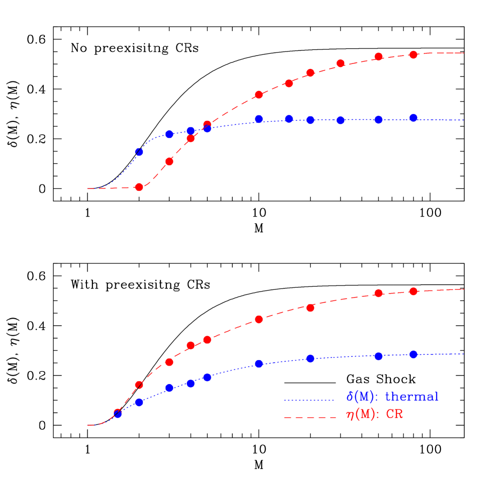
Figure 5: Gas thermalization efficiency, $\delta(M)$, and CR acceleration efficiency, $\eta(M)$, as a function of Mach number. Red and blue dots are the values estimated from numerical simulations based on a DSA model and red and blue lines are the fits. The top panel shows the case without preexisting CRs, while the bottom panel shows the case with preexisting CRs at a level of $P_{CR}/P_{g}\sim 0.3$ in the preshock region. Black solid line is for the gas thermalization efficiency for shocks without CRs.

References

- Beck & Kraus (2005) Beck, R., & Kraus, M. 2005, Astronomische Nachrichten, 326, 414
- Bell (1978) Bell A.R. 1978, MNRAS, 182, 147
- Biermann (1950) Biermann, L. 1950, Z. Naturforsch, A, 5, 65
- Berezhko et al. (1995) Berezhko, E. G., Ksenofontov, L. T., & Yelshin, V. K. 1995, Nucl. Phys. B, 39A, 171
- Berghöfer et al. (2000) Berghöfer, T. W., Bowyer, S., & Korpela, E. J. 2000, ApJ, 535, 615
- Binney (1974) Binney, J. 1974, MNRAS, 168, 73
- Blandford & Ostriker (1978) Blandford, R. D. & Ostriker, J. P. 1978, ApJ, 221, L29
- Blandford & Eichler (1987) Blandford, R. D. & Eichler, D. 1987, Phys. Rep., 154, 1
- Bowyer et al. (1999) Bowyer, S., Berghöfer, T. W., & Korpela, E. J. 1999, ApJ, 526, 592
- Cen & Ostriker (2006) Cen, R. & Ostriker, J. P. 2006, ApJ, 650, 560
- Cen et al. (2003) Cen, R., Ostriker, J. P., Prochaska, J. X., & Wolfe, A. M. 2003, ApJ, 598, 741
- Clarke (2004) Clarke, T. E., 2004, J. Korean Astron. Soc. 37, 337
- Clarke et al. (2001) Clarke, T. E., Kronberg, P. P., & Böhringer, H. 2001, ApJ, 547, L111
- Davies & Widrow (2000) Davies, G., & Widrow, L. M. 2000, ApJ, 540, 755
- Ellison et al. (1995) Ellison, D. C., Baring, M. G., & Jones, F. C. 1995, ApJ, 453, 873
- Fujita et al. (2003) Fujita, Y., Takizawa, M., & Sarazin, C. L. 2003, ApJ, 584, 190
- Fusco-Femiano et al. (1999) Fusco-Femiano, R., Dal Fiume, D., Feretti, L., Giovannini, G., Grandi, P., Matt, G., Molendi, S., & Santangelo, A. 1999, ApJ, 513, L21
- Gabici & Blasi (2003) Gabici, S. & Blasi, P. 2003, ApJ, 583, 695
- Giacalone et al. (1992) Giacalone, J., Burgess, D., Schwartz, S. J., & Ellison, D. C. 1992, Geophys. Res. Lett., 19, 433
- Giacalone (2005) Giacalone, J., 2005, ApJ, 628, L37
- Giovannini & Feretti (2000) Giovannini, G. & Feretti, L. 2000, New Astronomy, 5, 335
- Govoni & Feretti (2004) Govoni, F., & Feretti, L. 2004, International Journal of Modern Physics D, 13, 1549
- Inoue et al. (2007) Inoue, S., Sigl, G., Miniati, F., & Armengaud, E. 2007, preprint (astro-ph/0701167)
- Jokipii (1987) Jokipii, J. R. 1987, ApJ, 313, 842
- Kang & Jones (2003) Kang, H., 2003, J. Korean Astron. Soc., 36, 1
- Kang & Jones (2005) Kang, H. & Jones, T. W. 2005, ApJ., 620, 44
- Kang & Jones (2007) Kang, H. & Jones, T. W. 2007, in preparation
- Kang et al. (1997) Kang, H., Rachen, J. P., & Biermann, P. L. 1997, MNRAS, 286, 257
- Kang et al. (1996) Kang, H., Ryu, D., & Jones, T. W. 1996, ApJ, 456, 422
- Kronberg (1994) Kronberg, P. P. 1994, Rep. Prog. Phys. 57, 325
- Kronberg et al. (2004) Kronberg, P. P., Colgate, S. A., Li, H., & Dufton, Q. W. 2004, ApJ, 604, L77
- Kulsrud et al. (1997) Kulsrud, R. M., Cen, R., Ostriker, J. P., & Ryu, D. 1997, ApJ, 480, 481
- Li et al. (2006) Li, H., Lapenta, G., Finn, J. M., Li, S., & Colgate, S. A. 2006, ApJ, 643, 92
- Loeb & Waxmann (2000) Loeb, A. & Waxmann, E. 2000, Nature, 405, 156
- Longair (1994) Longair, M. S. 1994, High Energy Astrophysics, Volume 2 (London: Cambridge Univ. Press)
- Lucek & Bell (2000) Lucek, S. G. & Bell, A. R. 2000, MNRAS, 314, 65
- Malkov & Drury (2001) Malkov M.A. & Drury, L. O’C. 2001, Rep. Prog. Phys., 64, 429
- Medvedev et al. (2006) Medvedev, M. V., Silva, L. O., & Kamionkowski, M. 2006, ApJ, 642, L1
- Miniati et al. (2001a) Miniati, F., Jones, T. W., Kang, H., & Ryu. D. 2001a, ApJ, 562, 233
- Miniati et al. (2001b) Miniati, F., Ryu. D., Kang, H., & Jones, T. W. 2001b, ApJ, 559, 59
- Murgia et al. (2004) Murgia, M., Govoni, F., Feretti, L., Giovannini, G., Dallacasa, D., Fanti, R., Taylor, G. B., & Dolag, K. 2004, A&A, 424, 429
- Ostrowski & Siemieniec-Ozieblo (2002) Ostrowski, M. & Siemieniec-Ozieblo, G. 2002, A&Ap, 386, 829
- Pettini et al. (2002) Pettini, M., Ellison, S. L., Bergeron, J., & Petitjean, P. 2002, A&A, 391, 21
- Pfrommer et al. (2006) Pfrommer, C., Springel, V., Enßlin, T. A., & Jubelgas, M. 2006, MNRAS, 367, 113
- Reimer et al. (2003) Reimer, O., Pohl, M., Sreekumar, P., & Mattox, J. R. 2003, ApJ, 588, 155
- Ryu et al. (1998) Ryu, D., Kang, H., & Biermann, P. L. 1998, A&A, 335, 19
- Ryu et al. (2007) Ryu, D., Kang, H., Cho, J., & Das, S. 2007, in preparation (Paper II)
- Ryu et al. (2003) Ryu, D., Kang, H., Hallman, E., & Jones, T. W. 2003, ApJ, 593, 599 (Paper I)
- Ryu et al. (1993) Ryu, D., Ostriker, J. P., Kang, H., & Cen, R. 1993, ApJ, 414, 1
- Sarazin (1999) Sarazin, C. L. 1999, ApJ, 520, 529
- Schuecker et al. (2004) Schuecker, P., Finoguenov, A., Miniati, F., Böhringer, H., & Briel, U. G. 2004, A&A, 426, 387
- Subramanian et al. (2006) Subramanian, K., Shukurov, A., & Haugen, N. E. L. 2006, MNRAS, 366, 1437
- Vogt & Enßlin (2005) Vogt, C. & Enßlin, T. 2005, A&A, 434, 67
- Vök & Atoyan (1999) Völk, H. J. & Atoyan, A. M. 1999, Astroparticle Phys., 11, 73
- Weibel (1959) Weibel, E. S. 1959, Phys. Rev. Lett., 2. 83