Quasiparticles in Neon using the Faddeev Random Phase Approximation

Abstract

The spectral function of the closed-shell Neon atom is computed by expanding the electron self-energy through a set of Faddeev equations. This method describes the coupling of single-particle degrees of freedom with correlated two-electron, two-hole, and electron-hole pairs. The excitation spectra are obtained using the Random Phase Approximation, rather than the Tamm-Dancoff framework employed in the third-order algebraic diagrammatic contruction [ADC(3)] method. The difference between these two approaches is studied, as well as the interplay between ladder and ring diagrams in the self-energy. Satisfactory results are obtained for the ionization energies as well as the energy of the ground state with the Faddeev-RPA scheme that is also appropriate for the high-density electron gas.

I Introduction

Ab initio treatments of electronic systems become unworkable for sufficiently complex systems. On the other hand, the Kohn-Sham formulation Koh.65 of density functional theory (DFT) Hoh.64 incorporates many-body correlations (beyond Hartree-Fock), while only single-particle (sp) equations must be solved. Due to this simplicity DFT is the only feasible approach in some modern applications of electronic structure theory. There is therefore a continuing interest both in developing new and more accurate functionals and in studying conceptual improvements and extensions to the DFT framework. In particular it is found that DFT can handle short-range interelectronic correlations quite well, while there is room for improvements in the description of long-range (van der Waals) forces and dissociation processes.

Microscopic theories offer some guidance in the development of extensions to DFT. Orbital dependent functionals can be constructed using many-body perturbation theory (MBPT) Goe.94 ; Goe.05 . More recently, the development of general ab initio DFT Bar.05 ; Mor.05 addressed the lack of a systematic improvement in DFT methods. In this approach one considers an expansion of the exact ground-state wave function (e.g., MBPT or coupled cluster) from a chosen reference determinant. Requiring that the correction to the density vanishes at a certain level of perturbation theory allows one to construct the corresponding approximation to the Kohn-Sham potential.

A different route has been proposed in Ref. Van.06 by developing a quasi-particle (QP)-DFT formalism. In the QP-DFT approach the full spectral function is decomposed in the contribution of the QP excitations, and a remainder or background part. The latter part is complicated, but does not need to be known accurately: it is sufficient to have a functional model for the energy-averaged background part to set up a single-electron selfconsistency problem that generates the QP excitations. Such an approach is appealing since it contains the well-developed standard Kohn-Sham formulation of DFT as a special case, while at the same time emphasis is put on the correct description of QPs, in the Landau-Migdal sense Mig.67 . Hence, it can provide an improved description of the dynamics at the Fermi surface. Given the close relation between QP-DFT and the Green’s function (GF) formulation of many-body theory FetWal ; DicVan , it is natural to employ ab initio calculations in the latter formalism to investigate the structure of possible QP-DFT functionals. In this respect it is imperative to identify which classes of diagrams are responsible for the correct description of the QP physics.

Some previous calculations, based on GF theory, have focused on a self-consistent treatment of the self-energy at the second order Van.01 ; Pei.02 ; Dah.05 for simple atoms and molecules. For the atomic binding energies it was found that the bulk of correlations, beyond Hartree-Fock, are accounted for while significant disagreement with experiment persists for QP properties like ionization energies and electron affinities. The formalism beyond the second-order approximation was taken up in Ref. Ver.06 ; Shi.06 ; Dah.06 ; Dah.04 ; Sta.06 by employing a self-energy of the $GW$ type Hed.65 . In this approach, the random phase approximation (RPA) in the particle-hole (ph) channel is adopted to allow for possible collective effects on the atomic excited states. The latter are coupled to the sp states by means of diagrams like the last two in Fig. 1(c). Two variants of the $G_{0}W_{0}$ formalism were employed in Ref. Ver.06 (where the subscript “$0$” indicates that non-dressed propagators are used). In the first only the direct terms of the interelectron Coulomb potential are taken into account. In the second version, also the exchange terms are included when diagonalizing the ph space [generalized RPA (GRPA)] and in constructing the self-energy [generalized $GW$ ($GGW$)]. Although the exchange terms are known to be crucial in order to reproduce the experimentally observed Rydberg sequence in the excitation spectrum of neutral atoms, they were found to worsen the agreement between the theoretical and experimental ionization energies Ver.06 .

In the $GW$ approach the sp states are directly coupled with the two-particle–one-hole (2p1h) and the two-hole–one-particle (2h1p) spaces. However, only partial diagonalizations (namely, in the ph subspaces) are performed. This procedure unavoidably neglects Pauli correlations with the third particle (or hole) outside the subspace. In the case of the $GGW$ approach, this leads to a double counting of the second order self-energy which must be corrected for explicitly Fuk.64 ; Bar.06b . We note that simply subtracting the double counted diagram is not completely satisfactory here, since it introduces poles with negative residues in the self-energy. More important, the interaction between electrons in the two-particle (pp) and two-hole (hh) subspaces are neglected altogether in ($G$)$GW$. Clearly, it is necessary to identify which contributions, beyond $GGW$, are needed to correctly reproduce the QP spectrum.

In this respect, it is known that highly accurate descriptions of the QP properties in finite systems can be obtained with the algebraic diagrammatic construction (ADC) method of Schirmer and co-workers Sch.83 . The most widely used third-order version [ADC(3)] is equivalent to the so-called extended $2p1h$ Tamm-Dancoff (TDA) method Wal.81 and allows to predict ionization energies with an accuracy of 10-20 mH in atoms and small molecules. Upon inspection of its diagrammatic content, the ADC(3) self-energy is seen to contain all diagrams where TDA excitations are exchanged between the three propagator lines of the intermediate $2p1h$ or $2h1p$ propagation. The TDA excitations are constructed through a diagonalization in either $2p1h$ or $2h1p$ space, and neglect ground-state correlations. However, it is clear that use of TDA leads to difficulties for extended systems. In the high-density electron gas e.g., the correct plasmon spectrum requires the RPA in the $ph$ channel, rather than TDA.

In order to bridge the gap between the QP description in finite and extended systems, it seems therefore necessary to develop a formalism where the intermediate excitations in the $2p1h/2h1p$ propagator are described at the RPA level. This can be achieved by a formalism based on employing a set of Faddeev equations, as proposed in Ref. Bar.01 and subsequently applied to nuclear structure problems Bar.02 ; Dic.04 ; Bar.06 . In this approach the GRPA equations are solved separately in the ph and pp/hh subspaces. The resulting polarization and two-particle propagators are then coupled through an all-order summation that accounts completely for Pauli exchanges in the 2p1h/2h1p spaces. This Faddeev-RPA (F-RPA) formalism is required if one wants to couple propagators at the RPA level or beyond. Apart from correctly incorporating Pauli exchange, F-RPA takes the explicit inclusion of ground-state correlations into account, and can therefore be expected to apply to both finite and extended systems. The ADC(3) formalism is recovered as an approximation by neglecting ground-state correlations in the intermediate excitations (i.e. replacing RPA with TDA phonons).

In this work we consider the Neon atom and apply the F-RPA method to a nonrelativistic electronic problem for the first time. The relevant features of the F-RPA formalism (also extensively treated in Ref. Bar.01 ), are introduced in Sect. II. The application to the Neon atom is discussed in Sec. III, where we also investigate the separate effects of the ladder and ring series on the self-energy, as well as the differences between including TDA and RPA phonons. Our findings are summarized in Sec. IV. Some more technical aspects are relegated to the appendix, where the interested reader can find the derivation of the Faddeev expansion for the 2p1h/2h1p propagator, adapted from Ref. Bar.01 . In particular, the approach used to avoid the multiple-frequency dependence of the Green’s functions is discussed in App. A.1, along with its basic assumptions. The explicit expressions of the Faddeev kernels are given in App. A.3. Together with Ref. Bar.01 , the appendix provides sufficient information for an interested reader to apply the formalism.

II Formalism

The theoretical framework of the present study is that of propagator theory, where the object of interest is the sp propagator, instead of the many-body wave function. In this paper we will employ the convention of summing over repeated indices, unless specified otherwise. Given a complete orthonormal basis set of sp states, labeled by $\alpha$,$\beta$,…, the sp propagator can be written in its Lehmann representation as FetWal ; DicVan

$$g_{\alpha\beta}(\omega)~{}=~{}\sum_{n}\frac{\left({\cal X}^{n}_{\alpha}\right)^{*}\;{\cal X}^{n}_{\beta}}{\omega-\varepsilon^{+}_{n}+i\eta}~{}+~{}\sum_{k}\frac{{\cal Y}^{k}_{\alpha}\;\left({\cal Y}^{k}_{\beta}\right)^{*}}{\omega-\varepsilon^{-}_{k}-i\eta}\;,$$ (1)

where ${\cal X}^{n}_{\alpha}={\mbox{$\langle{\Psi^{N+1}_{n}}|$}}c^{{\dagger}}_{\alpha}{\mbox{$|{\Psi^{N}_{0}}\rangle$}}$  (${\cal Y}^{k}_{\alpha}={\mbox{$\langle{\Psi^{N-1}_{k}}|$}}c_{\alpha}{\mbox{$|{\Psi^{N}_{0}}\rangle$}}$) are the spectroscopic amplitudes, $c_{\alpha}$ ($c^{\dagger}_{\beta}$) are the second quantization destruction (creation) operators and $\varepsilon^{+}_{n}=E^{N+1}_{n}-E^{N}_{0}$ ($\varepsilon^{-}_{k}=E^{N}_{0}-E^{N-1}_{k}$). In these definitions, $|\Psi^{N+1}_{n}\rangle$, $|\Psi^{N-1}_{k}\rangle$ are the eigenstates, and $E^{N+1}_{n}$, $E^{N-1}_{k}$ the eigenenergies of the ($N\pm 1$)-electron system. Therefore, the poles of the propagator reflect the electron affinities and ionization energies.

The sp propagator solves the Dyson equation

$$g_{\alpha\beta}(\omega)=g^{0}_{\alpha\beta}(\omega)\;+\;g^{0}_{\alpha\gamma}(\omega)\Sigma^{\star}_{\gamma\delta}(\omega)g_{\delta\beta}(\omega)\;\;,$$ (2)

which depends on the irreducible self-energy $\Sigma^{\star}(\omega)$. The latter can be written as the sum of two terms

$$\Sigma^{\star}_{\alpha\beta}(\omega)~{}=~{}\Sigma^{HF}_{\alpha\beta}~{}+~{}\frac{1}{4}\,V_{\alpha\lambda,\mu\nu}~{}R_{\mu\nu\lambda,\gamma\delta\varepsilon}(\omega)~{}V_{\gamma\delta,\beta\varepsilon}\;,$$ (3)

where $\Sigma^{HF}$ represents the Hartree-Fock diagram for the self-energy. In Eqs. (2) and (3), $g^{0}(\omega)$ is the sp propagator for the system of noninteracting electrons, whose Hamiltonian contains only the kinetic energy and the electron-nucleus attraction. The $V_{\alpha\beta,\gamma\delta}$ represent the antisymmetrized matrix elements of the interelectron (Coulomb) repulsion. Note that in this work we only consider antisymmetrized elements of the interaction, hence, our result for the ring summation always compare to the generalized $GW$ approach. Equation (3) introduces the 2p1h/2h1p-irreducible propagator $R(\omega)$, which carries the information concerning the coupling of sp states to more complex configurations. Both $\Sigma^{\star}(\omega)$ and $R(\omega)$ have a perturbative expansion as a power series in the interelectron interaction ${\hat{V}}$. Some of the diagrams appearing in the expansion of $R(\omega)$ are depicted in Fig. 1, together with the corresponding contributions to the self-energy. Note that already at zero order in $R(\omega)$ (three free lines with no mutual interaction) the second order self-energy is generated.

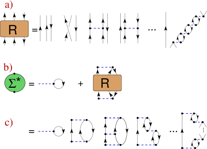
Figure 1: (Color online) a) Diagrammatic expansion of $R(\omega)$ in terms of the (antisymmetrized) Coulomb interaction and undressed propagators. b) $R(\omega)$ is related to the self-energy according to Eq. (3). c) By substituting the diagrams a) in the latter equation, one finds the perturbative expansion of the self-energy.

Different approximations to the self-energy can be constructed by summing particular classes of diagrams. In this work we are interested in the summation of rings and ladders, through the (G)RPA equations. In order to include such effects in $R(\omega)$, we first consider the polarization propagator describing excited states in the $N$-electron system

$$\Pi_{\alpha\beta,\gamma\delta}(\omega) = \sum_{n\neq 0}\frac{{\mbox{$\langle{\Psi^{N}_{0}}|$}}c^{{\dagger}}_{\beta}c_{\alpha}{\mbox{$|{\Psi^{N}_{n}}\rangle$}}\;{\mbox{$\langle{\Psi^{N}_{n}}|$}}c^{{\dagger}}_{\gamma}c_{\delta}{\mbox{$|{\Psi^{N}_{0}}\rangle$}}}{\omega-\left(E^{N}_{n}-E^{N}_{0}\right)+i\eta}$$ (4)

$$- \sum_{n\neq 0}\frac{{\mbox{$\langle{\Psi^{N}_{0}}|$}}c^{{\dagger}}_{\gamma}c_{\delta}{\mbox{$|{\Psi^{N}_{n}}\rangle$}}\;{\mbox{$\langle{\Psi^{N}_{n}}|$}}c^{{\dagger}}_{\beta}c_{\alpha}{\mbox{$|{\Psi^{N}_{0}}\rangle$}}}{\omega+\left(E^{N}_{n}-E^{N}_{0}\right)-i\eta}\;,$$

and the two-particle propagator, that describes the addition/removal of two electrons

$$g^{II}_{\alpha\beta,\gamma\delta}(\omega) = \sum_{n}\frac{{\mbox{$\langle{\Psi^{N}_{0}}|$}}c_{\beta}c_{\alpha}{\mbox{$|{\Psi^{N+2}_{n}}\rangle$}}\;{\mbox{$\langle{\Psi^{N+2}_{n}}|$}}c^{{\dagger}}_{\gamma}c^{{\dagger}}_{\delta}{\mbox{$|{\Psi^{N}_{0}}\rangle$}}}{\omega-\left(E^{N+2}_{n}-E^{N}_{0}\right)+i\eta}$$ (5)

$$- \sum_{k}\frac{{\mbox{$\langle{\Psi^{N}_{0}}|$}}c^{{\dagger}}_{\gamma}c^{{\dagger}}_{\delta}{\mbox{$|{\Psi^{N-2}_{k}}\rangle$}}\;{\mbox{$\langle{\Psi^{N-2}_{k}}|$}}c_{\beta}c_{\alpha}{\mbox{$|{\Psi^{N}_{0}}\rangle$}}}{\omega-\left(E^{N}_{0}-E^{N-2}_{k}\right)-i\eta}\;.$$

We note that the expansion of $R(\omega)$ arises from applying the equations of motion to the sp propagator (1), which is associated to the ground state $|\Psi^{N}_{0}\rangle$. Hence, all the Green’s functions appearing in this expansion will also be ground state based, including Eqs. (4) and (5). However the latter contain, in their Lehmann representations, all the relevant information regarding the excitation of ph and pp/hh collective modes. The approach of Ref. Bar.01 consists in computing these quantities by solving the ring-GRPA and the ladder-RPA equations DicVan , which are depicted for propagators in Fig. 2. In the more general case of a self-consistent calculation, a fragmented input propagator can be used and the corresponding dressed (G)RPA [D(G)RPA] equations DicVan ; Geu.94 solved [see Eqs. (10) and (10)]. Since the propagators (4) and (5) reflect two-body correlations, they still have to be coupled to an additional sp propagator in order to obtain the corresponding approximation for the 2p1h and 2h1p components of $R(\omega)$. This is achieved by solving two separate sets of Faddeev equations.

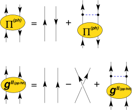
Figure 2: (Color online) Diagrammatic equations for the polarization (above) and the two-particle (below) propagators in the (G)RPA approach. Dashed lines are always antisymmetrized Coulomb matrix elements and the full lines represent free (undressed) propagators.

Taking the 2p1h case as an example, one can split $R^{(2p1h)}(\omega)$ in three different components $\bar{R}^{(i)}(\omega)$ ($i=1,2,3$) that differ from each other by the last pair of lines that interact in their diagrammatic expansion,

$$\bar{R}^{(2p1h)}_{\alpha\beta\gamma,\mu\nu\lambda}(\omega)=\left[{G^{0}}^{>}_{\alpha\beta\gamma,\mu\nu\lambda}(\omega)-{G^{0}}^{>}_{\beta\alpha\gamma,\mu\nu\lambda}(\omega)\right]+\sum_{i=1,2,3}\bar{R}^{(i)}_{\alpha\beta\gamma,\mu\nu\lambda}(\omega)\;,$$ (6)

where ${G^{0}}^{>}(\omega)$ is the 2p1h propagator for three freely propagating lines. These components are solutions of the following set Faddeev equations Fad.61

$$\bar{R}^{(i)}_{\alpha\beta\gamma,\mu\nu\lambda}(\omega)~{}=~{}{G^{0}}^{>}_{\alpha\beta\gamma,\mu^{\prime}\nu^{\prime}\lambda^{\prime}}(\omega)~{}\Gamma^{(i)}_{\mu^{\prime}\nu^{\prime}\lambda^{\prime},\mu^{\prime\prime}\nu^{\prime\prime}\lambda^{\prime\prime}}(\omega)$$

$$\times ~{}\left[\bar{R}^{(j)}_{\mu^{\prime\prime}\nu^{\prime\prime}\lambda^{\prime\prime},\mu\nu\lambda}(\omega)~{}+~{}\bar{R}^{(k)}_{\mu^{\prime\prime}\nu^{\prime\prime}\lambda^{\prime\prime},\mu\nu\lambda}(\omega)\right.$$

$$~{}~{}+~{}\left.{G^{0}}^{>}_{\mu^{\prime\prime}\nu^{\prime\prime}\lambda^{\prime\prime},\mu\nu\lambda}(\omega)-{G^{0}}^{>}_{\nu^{\prime\prime}\mu^{\prime\prime}\lambda^{\prime\prime},\mu\nu\lambda}(\omega)\right]\;,~{}~{}i=1,2,3~{}$$

where ($i,j,k$) are cyclic permutations of ($1,2,3$). The interaction vertices $\Gamma^{(i)}(\omega)$ contain the couplings of a ph or pp/hh collective excitation and a freely propagating line. These are given in the Appendix in terms of the polarization (4) and two-particle (5) propagators. Equations. (II) include RPA-like phonons and fully describe the resulting energy dependence of $R(\omega)$. However, they still neglect energy-independent contributions–even at low order in the interaction–that also correspond to relevant ground-state correlations. The latter can be systematically inserted according to

$$R^{(2p1h)}_{\alpha\beta\gamma,\mu\nu\lambda}(\omega)~{}=~{}U_{\mu\nu\lambda,\mu^{\prime}\nu^{\prime}\lambda^{\prime}}\;\bar{R}^{(2p1h)}_{\mu^{\prime}\nu^{\prime}\lambda^{\prime},\mu^{\prime\prime}\nu^{\prime\prime}\lambda^{\prime\prime}}(\omega)\;U^{\dagger}_{\mu^{\prime\prime}\nu^{\prime\prime}\lambda^{\prime\prime},\mu\nu\lambda}\;,$$ (8)

where $R(\omega)$ is the propagator we employ in Eq. (3), $\bar{R}(\omega)$ is the one obtained by solving Eqs. (II), ${\bf U}\equiv{\bf I}+\Delta{\bf U}$, and $\bf I$ is the identity matrix. Following the algebraic diagrammatic construction method Wal.81 ; Sch.83 , the energy independent term $\Delta\bf U$ was determined by expanding Eq. (8) in terms of the interaction and imposing that it fulfills perturbation theory up to first order (corresponding to third order in the self-energy). The resulting $\Delta\bf U$, employed in this work, is the same as in Ref. Wal.81 and is reported in App. A.3 for completeness. It has been shown that the additional diagrams introduced by this correction are required to obtain accurate QP properties. Equations. (II) and (8) are valid only in the case in which a mean-field propagator is used to expand $R(\omega)$. This is the case of the present work, which employs Hartree-Fock sp propagators as input. The derivation of these equations for the general case of a fragmented propagator is given in the appendix. More details about the actual implementation of the Faddeev formalism to 2p1h/2h1p propagation have been presented in Ref. Bar.01 . The calculation of the 2h1p component of $R(\omega)$ follows completely analogous steps.

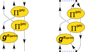
Figure 3: (Color online) Example of one of the diagrams that are summed to all orders by means of the Faddeev Eqs. (II) (left). The corresponding contribution to the self-energy, obtained upon insertion into Eq. (3), is also shown (right).

It is important to note that the present formalism includes the effects of ph and pp/hh motion to be included simultaneously, while allowing interferences between these modes. These excitations are evaluated here at the RPA level and are then coupled to each other by solving Eqs. (II). This generates diagrams as the one displayed in Fig. 3, with the caveat that two phonons are not allowed to propagate at the same time. Equations. (II) also assure that Pauli correlations are properly taken into account at the 2p1h/2h1p level. In addition, one can in principle employ dressed sp propagators in these equations to generate a self-consistent solution. If we neglect the ladder propagator $g^{II}(\omega)$ (5) in this expansion, we are left with the ring series alone and the analogous physics ingredients as for the generalized $GW$ approach. However, this differs from $GGW$ due to the fact that no double counting of the second-order self-energy occurs, since the Pauli exchanges between the polarization propagator and the third line are properly accounted for (see Fig. 3). Alternatively, one can suppress the polarization propagator to investigate the effects of pp/hh ladders alone.

It is instructive to replace in the above equations all RPA phonons with TDA ones; this amounts to allowing only forward-propagating diagrams in Fig. 2, and is equivalent to separate diagonalisations in the spaces of $ph$, $pp$ and $hh$ configurations, relative to the HF ground state. It can be shown that using these TDA phonons to sum all diagrams of the type in Fig. 3 reduces to one single diagonalization in the $2p1h$ or $2h1p$ spaces. Therefore, Eqs. (II) and (8) with TDA phonons lead directly to the “extended” $2p1h$ TDA of Ref. Wal.81 , which was later shown to be equivalent to ADC(3) in the general ADC framework Sch.83 . The Faddeev expansion formalism of Ref. Bar.01 creates the possibility to go beyond ADC(3) by including RPA phonons. This is more satisfactory in the limit of large systems. At the same time, the computational cost remains modest since only diagonalizations in the $2p1h/2h1p$ spaces are required.

Note that complete self-consistency requires the use of fragmented (or dressed) propagators in the evaluation of all ingredients leading to the self-energy. This is outside the scope of the present paper, but we included partial selfconsistency by taking into account the modifications to the HF diagram by employing the correlated one-body density matrix and iterating to convergence. This is relatively simple to achieve, since the $2p1h/2h1p$ propagator is only evaluated once with the input HF propagators. Below we will give results with and without this partial selfconsistency at the HF level.

$l$		0	1	2	3	4	5	6
$r_{w}$		2.0	4.0	0.0	0.0	0.0	0.0	0.0
$n_{o}$		12	21	10	10	5	5	5

Table 1: Parameters that define the sp basis: radius of the confining wall $r_{w}$ (in atomic units) and number of orbits $n_{o}$ used for different partial waves $l$. The value of $c_{w}$ is always set to 5 a.u..

III Results

Calculations have been performed using two different model spaces: (1) a standard quantumchemical Gaussian basis set, aug-cc-pVTZ for Neon Dunning , with Cartesian representation of the $d$ and $f$ functions; (2) a numerical basis set based on HF and subsequent discretization of the continuum, to be detailed below. The aug-cc-pVTZ basis set was used primarily to check our formalism with the ADC(3) result in literature (i.e. Tro.05 , where this basis was employed). The HF+continuum basis allows to approach, at least for the ionization energies, the results for the full sp space (basis set limit).

The HF+continuum is the same discrete model space employed previously in Refs. Van.01 ; Ver.06 . It consists of: (1) Solving on a radial grid the HF problem for the neutral atom; (2) Adding to this fixed nonlocal HF potential a parabolic potential wall of the type $U(r)=\theta(r-r_{w})c_{w}(r-r_{w})^{2}$, placed at a distance $r_{w}$ of the nucleus. The latter eigenvalue problem has a basis of discrete eigenstates. This basis is truncated by specifying some largest angular momentum $l_{\mbox{max}}$ and the number of virtual states for each value of $l\leq l_{\mbox{max}}$. (3) Solve the HF problem again, without the potential wall, in this truncated discrete space. The resulting basis set is used for the subsequent Green’s function calculations.

When a sufficiently large number of states is retained after truncation, the final results should approach the basis set limit. In particular the results should not depend on the choice of the auxiliary confining potential. This was verified in Ref. Van.01 for the second-order, and in Ref. Ver.06 for the $G_{0}W_{0}$ self-energy; in these cases the self-energy is sufficiently simple that extensive convergence checks can be made for various choices of the auxiliary potential. The parameters of the confining wall and the number of sp states kept in the basis set was optimized in Ref. Van.01 , by requiring that the ionization energy is converged to about 1 mH for the second-order self-energy. In Ref. Ver.06 the same choice of basis set was also seen to bring the ionization energy for the $G_{0}W_{0}$ self-energy near convergence. For completeness, the details of this basis are reported in Table 1. While the self-energy in the present paper is too complicated to allow similar convergence checks, it seems safe to assume that basis set effects will affect the calculated ionization energies by at most 5 mH.

	F-TDA	F-RPA	F-TDAc	F-RPAc	Expt.
2p	-0.799	-0.791	-0.803	-0.797 (0.94)	-0.793 (0.92)
2s	-1.796	-1.787	-1.802	-1.793 (0.90)	-1.782 (0.85)
1s	-32.126	-32.087	-32.140	-32.102 (0.86)	-31.70
$E_{\mbox{tot}}$	-128.778	-128.772	-128.836	-128.840	-128.928

Table 2: Results with the aug-cc-pVTZ basis. The first three rows list the energies of the main sp fragments below the Fermi level, as predicted by different self-energies. F-TDA/F-RPA refers to the Faddeev summation with TDA/RPA phonons, respectively. In all cases the self-energy was corrected at third order through Eq. (8). The suffix “c” refers to partial selfconsistency, when the static (HF-type) self-energy is consistent with the correlated density matrix. Without “c” the pure HF self-energy was taken. In the F-RPAc column the strength of the fragment is indicated between brackets. The last row is the total electronic binding energy. The experimental values are taken from Refs. NIST ; Tho.01 . All energies are in atomic units.

In Table 2 we compare, for the aug-cc-pVTZ basis, the ionization energies of the main single-hole configurations when TDA or RPA phonons are employed in the Faddeev construction (this is labeled F-TDA and F-RPA, respectively, in the table). Note that use of TDA phonons corresponds to the usual ADC(3) self-energy. We find that the replacement of TDA with RPA phonons provides more screening, leading to slightly less bound poles which are shifted towards the experimental values. This shift increases with binding energy. As discussed at the end of Sec. I, one can include consistency of the static part of the self-energy. About eight iterations are needed for convergence. This is a nonnegligible correction, providing about 5 mH more binding (i.e. larger ionization energies) for the valence/subvalence $2p$ and $2s$, 15 mH for the deeply bound $1s$, and 60 mH to the total binding energy. Our converged result for the Faddeev-TDA self-energy (labeled F-TDAc in Table 2) is in good agreement with the ADC(3) value for the $2p$ ionization energy (-0.804 H) quoted in Tro.05 , as it should be.

The analogous results obtained with the larger HF+continuum basis are given in Table 3, which allows to assess overall stability and basis set effects. We find exactly the same trends as for aug-cc-pVTZ. In particular the reduction of ionization energies from the replacement of TDA with RPA phonons is almost independent of the basis set used, while the effect of including partial consistency is roughly halved. Overall, the ionization states are always more bound with the larger basis set; while the basis set limit could be still more bound than the present results with the HF+continuum basis set, it is likely (based on the $G_{0}W_{0}$ extrapolation in Ref. Ver.06 ) that the difference does not exceed 5 mH.

	F-TDA	F-RPA	F-TDAc	F-RPAc	Expt.
2p	-0.807	-0.799	-0.808	-0.801 (0.94)	-0.793 (0.92)
2s	-1.802	-1.792	-1.804	-1.795 (0.91)	-1.782 (0.85)
1s	-32.136	-32.097	-32.142	-32.104 (0.81)	-31.70
$E_{\mbox{tot}}$	-128.863	-128.857	-128.883	-128.888	-128.928

Table 3: Results with the HF+continuum basis set from Table 1. See also the caption of Table 2.

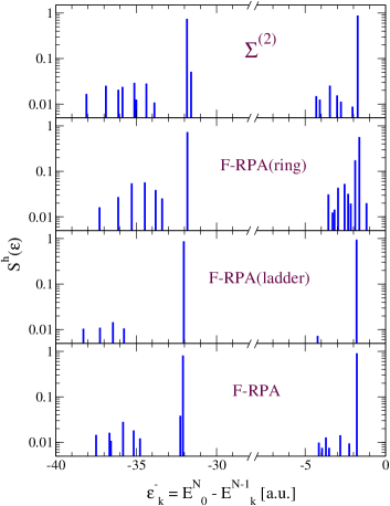
Figure 4: (Color online) Spectral function for the $s$ states in Ne obtained with various self-energy approximations. From the top down: the second-order ($\Sigma^{(2)}$) self-energy, the F-RPA(ring), the F-RPA(ladder), and the full F-RPA self-energy. The strength is given relative to the Hartree-Fock occupation of each shell. Only fragments with strength larger than $Z>0.005$ are shown.

	1s	2s	2p
HF	-32.77 (1.00)	-1.931 (1.00)	-0.850 (1.00)
$\Sigma^{(2)}$	-31.84 (0.74)	-1.736 (0.88)	-0.747 (0.91)
$G_{0}W_{0}$	-31.14 (0.85)	-1.774 (0.91)	-0.801 (0.94)
F-RPA (ring)	-31.82 (0.73)	-1.636 (0.56)	-0.730 (0.80)
F-RPA (ladder)	-32.04 (0.87)	-1.802 (0.95)	-0.781 (0.96)
F-RPA	-32.10 (0.81)	-1.792 (0.91)	-0.799 (0.94)
Exp.	-31.70	-1.782 (0.85)	-0.793 (0.92)

Table 4: Energy (in a.u.) and strength (bracketed numbers) of the main fragments in the spectral function of Neon, generated by different self-energies. Results for the HF+continuum basis. Consecutive rows refer to: (1) HF; (2) second-order self-energy; (3) $G_{0}W_{0}$ results from Ref. Ver.06 ; (4) F-RPA self-energy with only $ph$ rings retained; (5) F-RPA self-energy with only $pp/hh$ ladders retained; (6) Complete F-RPA self-energy. In all F-RPA results the self-energy was corrected at third order through Eq. (8). The static self-energy was pure HF (no partial self-consistency). The experimental values are taken from Refs. NIST ; Tho.01 .

.

As discussed in Sec. I, the the F-RPA self-energy contains RPA excitations of both $ph$ type (ring diagrams) and $pp/hh$ type (ladder diagrams). It is instructive to analyze their separate contributions to the final ionization energies, in order to understand how the F-RPA self-energy is related to the standard $(G)GW$ self-energy. Table 4 compares the results for the ionization energies, obtained with the second-order self-energy, to different approximations for including the ring summations. As one can see, the second-order self-energy generates an $l$=1 sp energy of -0.747 mH, which is 46 mH above the empirical $2p$ ionization energy. The $G_{0}W_{0}$ self-energy, which includes the ring summation with only direct Coulomb matrix elements, improves this result and brings it close to experiment. The $2s$ behaves in a similar way. Unfortunately, including the exchange terms of the interelectron repulsion in the $GG_{0}W_{0}$ method turns out to have the opposite effect (the $2p$ ionization energy becomes -0.712 H  Ver.06 ) and the agreement with experiment is lost. Obviously, $GG_{0}W_{0}$ is too simplistic to account for exchange in the $ph$ channel.

With the F-RPA(ring) self-energy one can go one step further and employ the Faddeev expansion to also force proper Pauli exchange correlations in the 2p1h/2h1p spaces. As shown in Table 4, this enhances the screening due to the exchange interaction terms, leading to even less binding for the $2s$ and $2p$. The corrections relative to the second-order self-energy can be large (100 mH for the $2s$ state) and in the direction away from the experimental value. We also note that the larger shift, in the 2$s$ orbit, is accompanied by an increase of the fragmentation (see Fig. 4 and Tab. 4). Similar observations were also made in Ref. Ver.06 for other atoms: in general ring summations in the direct channel alone bring the quasihole peaks close to the experiment. This agreement is then spoiled as soon as one includes proper exchange terms in the self-energy. On the other hand, exchange in the ph channel is required to reproduce the correct Rydberg sequence in the excitation spectrum of neutral atoms. So further corrections must arise from other diagrams, and obviously the summation of ladder diagrams can play a relevant role, since these contribute to the expansion of the self-energy at the same level as that of the ring diagrams.

The result when only including ladder-type RPA phonons in the F-RPA self-energy is also shown in Table 4. One can see that pp/hh ladders do actually work in the opposite way as the ph channel ring diagrams, and have the same order of magnitude with, e.g., a shift of 66 mH for the $2s$ relative to the second-order result. When combined with the ring diagrams in the full F-RPA self-energy, the agreement with experiment is restored again. Note that the final result cannot be obtained by adding the contributions of rings and ladders, but depends nontrivially on the interplay between these classes of diagrams thereby pointing to significant interference effects.

With the F-RPA(ring) self-energy, where only the contributions of the $ph$ channel are included, the main peaks listed in Table 4 are not only considerably shifted but also strongly depleted, e.g. a strength of only 0.56 for the main $2s$ peak. The complete spectral function for the $l=0$ strength in Fig. 4 shows that the depletion of the main fragment is accompanied by strong fragmentation over several states. While correlation effects are overestimated in F-RPA(ring), they are suppressed in F-RPA(ladder), where only the $pp/hh$ ladders are included in the self-energy. In this case one finds a spectral distribution closer to the HF one, with a main $2s$ fragment of strength 0.95 and less fragmentation than the the second-order self-energy. The spectral distribution generated by the complete F-RPA self-energy is again a combination of the above effects. The strength of the deeply bound $1s$ orbital behaves in an analogous way. The strength of the main peak is reduced but several satellite levels appear due to the mixing with $2h1p$ configurations. In all the calculations reported in Fig. 4 we found a summed $l=0$ strength exceeding 0.98 in the interval [-40 H, -30 H] which can be associated with the $1s$ orbital, and this remains true even in the presence of strong correlations using the F-RPA(ring) self-energy. Of course, the mixing with $3h2p$ configurations, not included in this work, may further contribute to the fragmentation pattern in this energy region.

IV Conlusions and discussion

In conclusion, the electronic self-energy for the Ne atom was computed by the F-RPA method which includes –simultaneously– the effects of both ring and ladder diagrams. This was accomplished by employing an expansion of the self-energy based on a set of Faddeev equations. This technique was originally proposed for nuclear structure applications Bar.01 and is described in the appendix. At the level of the self-energy one sums all diagrams where the three propagator lines of the intermediate $2p1h$ or $2h1p$ propagation are connected by repeated exchange of RPA excitations in both the $ph$ and the $pp/hh$ channel. This differs from the ADC(3) formalism in the fact that the exchanged excitations are of the RPA type, rather than the TDA type, and therefore take ground-state correlations effects into account. The coupling to the external points of the self-energy uses the same modified vertex as in ADC(3), which must be introduced to include consistently all third-order perturbative contributions.

The resulting main ionization energies in the Neon atom are at least of the same quality, and even somewhat improved, compared to the ADC(3) result. Note that, numerically, F-RPA can be implemented as a diagonalization in $2p1h/2h1p$ space implying about the same cost as ADC(3). The present study also shows that in localized electronic systems subtle cancellations occur between the ring and ladder series. In particular, only a combination of the ring and ladder series leads to sensible results, as the separate ring series tends to correct the second-order result in the wrong direction.

Since the limit to extended systems requires an RPA treatment of excitations, the F-RPA method holds promise to bridge the gap between an accurate description of quasiparticles in both finite and extended systems. In particular, the $GW$ treatment of the electron gas has been shown to yield excellent binding energies, but poor quasiparticle properties Holm ; Godby . Further progress beyond $GW$ theory requires a consistent incorporation of exchange in the $ph$ channel. The F-RPA technique may be highly relevant in this respect. A common framework for calculating accurate QP properties in both finite and extended systems, is also important for constraining functionals in quasiparticle density functional theory (QP-DFT) Van.06 .

Finally, complete self-consistency requires sizable computational efforts for bases as large as the HF+continuum basis used here. It would nevertheless represent an important extension of the present work, since it is related to the fulfillment of conservation laws Bay.61 ; Bay.62 . These issues will be addressed in future work.

Appendix A Faddeev expansion of the 2p1h/2h1p propagator

Although only the one-energy (or two-time) part of the 2p1h/2h1p propagator enters the definition of the self energy, Eq. (3), a full resummation of all its diagrammatic contributions would require to treat explicitly the dependence on three separate frequencies, corresponding to the three final lines in the expansion of $R(\omega)$. For example, inserting the RPA ring (ladder) series in $R(\omega)$ implies the propagation of a ph (pp/hh) pair of lines both forward and backward in time, while the third line remains unaffected. A way out of this situation is to solve the Bethe-Salpeter-like equations for the polarization and ladder propagators separately and then to couple them to the additional line. If it is assumed that different phonons do not overlap in time, the three lines in between phonon structures will propagate only in one time direction [see figures (3) and (5)]. In this situation the integration over several frequencies can be circumvented following the prescription detailed in the next subsection. This approach will be discussed in the following for the general case of a fully fragmented propgator, in order to derive a set of Faddeev equations capable of dressing the sp propagator self-consistently. Since the forward (2p1h) and the backward (2h1p) parts of $R(\omega)$ decouple in two analogous sets of equations, it is sufficient to focus on the first case alone.

A.1 Multiple frequencies integrals

Figure 5: (Color online) Diagrammatic representation of Eq. (A.1). Double lines represent fully dressed sp Green’s funcions which, however, are restricted to propagate only in one time direction [i.e., only one of the two terms on the r.h.s. of Eq. (1) is retained]. The Faddeev Eqs. (20) and (II) allow for both forward and backward propagation of the phonons $\Gamma^{(\pi)}(\omega)$ and $\Gamma^{(II)}(\omega)$ as long as these do not overlap in time. For the propagators, time ordereing is asumed with forwad propagation in the upward direction.

We start by considering the effective interactions in the ph and pp/hh channels that correspond to Eqs. (4) and (5) stripped of the external legs. In the present work, these are the following two-time objects:

$$\Gamma^{(\pi)}_{\alpha\beta,\gamma\delta}(\omega) = V_{\alpha\delta,\beta\gamma}~{}+~{}V_{\alpha\nu,\beta\mu}\;\Pi^{II}_{\mu\nu,\rho\sigma}(\omega)\;V_{\rho\delta,\sigma\gamma}$$

$$= V_{\alpha\delta,\beta\gamma}~{}+~{}\sum_{n}\frac{\left(\Omega^{n}_{\alpha\beta}\right)^{*}\;\Omega^{n}_{\gamma\delta}}{\omega-\varepsilon^{\pi}_{n}+i\eta}~{}-~{}\sum_{n^{\prime}}\frac{\Omega^{n^{\prime}}_{\beta\alpha}\;\left(\Omega^{n^{\prime}}_{\delta\gamma}\right)^{*}}{\omega+\varepsilon^{\pi}_{n^{\prime}}-i\eta}\;,$$

$$\Gamma^{(II)}_{\alpha\beta,\gamma\delta}(\omega) = V_{\alpha\beta,\gamma\delta}~{}+~{}V_{\alpha\beta,\mu\nu}\;g^{II}_{\mu\nu,\rho\sigma}(\omega)\;V_{\rho\sigma,\gamma\delta}$$

$$= V_{\alpha\delta,\beta\gamma}~{}+~{}\sum_{n}\frac{\left(\Delta^{+,n}_{\alpha\beta}\right)^{*}\;\Delta^{+,n}_{\gamma\delta}}{\omega-\varepsilon^{\Gamma+}_{n}+i\eta}~{}-~{}\sum_{k}\frac{\Delta^{-,k}_{\alpha\beta}\;\left(\Delta^{-,k}_{\gamma\delta}\right)^{*}}{\omega-\varepsilon^{\Gamma-}_{k}-i\eta}\;,$$

where the residues and poles for the ring series are $\Omega^{n}_{\alpha\beta}=\langle\Psi^{N}_{n}|c^{{\dagger}}_{\mu}c_{\nu}|\Psi^{N}_{0}\rangle V_{\mu\beta,\nu\alpha}$ and $\varepsilon^{\pi}_{n}=E^{N}_{n}-E^{N}_{0}$. For the ladders, $\Delta^{+,n}_{\alpha\beta}=\langle\Psi^{N+2}_{n}|c^{{\dagger}}_{\mu}c^{{\dagger}}_{\nu}|\Psi^{N}_{0}\rangle V_{\mu\nu,\alpha\beta}$ and $\Delta^{-,k}_{\alpha\beta}=V_{\alpha\beta,\mu\nu}\langle\Psi^{N-2}_{k}|c_{\mu}c_{\nu}|\Psi^{N}_{0}\rangle$, with poles $\varepsilon^{\Gamma+}_{n}=E^{N+2}_{n}-E^{N}_{0}$ and $\varepsilon^{\Gamma-}_{k}=E^{N}_{0}-E^{N-2}_{k}$. Equations. (9) solve the ring and ladder RPA equations, respectively

$$\Gamma^{(\pi)}_{\alpha\beta,\gamma\delta}(\omega) = V_{\alpha\delta,\beta\gamma}$$

$$+ \Gamma^{(\pi)}_{\alpha\beta,\mu\nu}(\omega)\;\int\frac{d\omega_{1}}{2\pi i}g_{\mu\rho}(\omega+\omega_{1})g_{\sigma\nu}(\omega_{1})\;V_{\rho\delta,\sigma\gamma}\;,$$

$$\Gamma^{(II)}_{\alpha\beta,\gamma\delta}(\omega) = V_{\alpha\beta,\gamma\delta}$$

$$+ \Gamma^{(II)}_{\alpha\beta,\mu\nu}(\omega)\;\frac{1}{2}\int\frac{d\omega_{1}}{-2\pi i}g_{\mu\rho}(\omega-\omega_{1})g_{\nu\sigma}(\omega_{1})\;V_{\rho\sigma,\gamma\delta}\;.$$

To display how the phonons (9) and (9) enter the expansion of $R(\omega)$, we perform explicitly the frequency integrals for the diagram of Fig. 5. Since it is assumed that the separate propagators lines evolve only in one time direction, only the forwardgoing ($g^{>}(\omega)$) or the backwardgoing ($g^{<}(\omega)$) part of Eq. (1) must be included for particles and holes, respectively. After some algebra, one obtains

$$\Delta R_{\alpha\beta\gamma,\mu\nu\lambda}(\omega)~{}=~{}\int\frac{d\omega_{1}}{2\pi i}\,\frac{d\omega_{2}}{2\pi i}\,\frac{ds}{2\pi i}\,\frac{d\Omega}{2\pi i}$$

$$\hskip 28.45274pt\;g^{>}_{\alpha\alpha_{1}}(\omega-\Omega)\;g^{>}_{\beta\beta_{1}}(\omega_{1})\;g^{<}_{\gamma_{1}\gamma}(\omega_{1}-\Omega)\;\Gamma^{(\pi)}_{\beta_{1}\gamma_{1},\sigma_{1}\lambda_{1}}(\Omega)\;g^{>}_{\sigma_{1}\sigma_{2}}(s+\Omega-\omega)\;\frac{1}{2}\Gamma^{(II)}_{\alpha_{1}\sigma_{2},\mu_{1}\nu_{1}}(s)\;g^{>}_{\mu_{1}\mu}(s-\omega_{2})\;g^{>}_{\nu_{1}\nu}(\omega_{2})\;g^{<}_{\lambda\lambda_{1}}(s-\omega)$$

$$= \frac{\left({\cal X}^{n_{1}}_{\alpha}{\cal X}^{n_{2}}_{\beta}{\cal Y}^{k_{3}}_{\gamma}\right)^{*}\;{\cal X}^{n_{1}}_{\alpha_{1}}{\cal X}^{n_{2}}_{\beta_{1}}{\cal Y}^{k_{3}}_{\gamma_{1}}}{\omega-(\varepsilon^{+}_{n_{1}}+\varepsilon^{+}_{n_{2}}-\varepsilon^{-}_{k_{3}})+i\eta}\;\left\{V_{\beta_{1}\lambda_{1},\gamma_{1}\sigma_{1}}~{}+~{}\frac{\left(\Omega^{n_{\pi}}_{\beta_{1}\gamma_{1}}\right)^{*}\Omega^{n_{\pi}}_{\sigma_{1}\lambda_{1}}}{\omega-(\varepsilon^{+}_{n_{1}}+\varepsilon^{\pi}_{n_{\pi}})+i\eta}~{}+~{}\frac{[\omega-\varepsilon^{\pi}_{n^{\prime}_{\pi}}-\varepsilon^{+}_{n_{1}}-\varepsilon^{+}_{n_{2}}+\varepsilon^{-}_{k_{3}}-\varepsilon^{+}_{n_{4}}+\varepsilon^{-}_{k_{7}}]\;\Omega^{n^{\prime}_{\pi}}_{\gamma_{1}\beta_{1}}\left(\Omega^{n^{\prime}_{\pi}}_{\lambda_{1}\sigma_{1}}\right)^{*}}{[-\varepsilon^{\pi}_{n^{\prime}_{\pi}}-\varepsilon^{+}_{n_{2}}+\varepsilon^{-}_{k_{3}}][-\varepsilon^{\pi}_{n^{\prime}_{\pi}}-\varepsilon^{+}_{n_{4}}+\varepsilon^{-}_{k_{7}}]}\right\}$$

$$\times~{}\frac{\left({\cal X}^{n_{4}}_{\sigma_{1}}\right)^{*}\;{\cal X}^{n_{4}}_{\sigma_{2}}}{\omega-(\varepsilon^{+}_{n_{1}}+\varepsilon^{+}_{n_{4}}-\varepsilon^{-}_{k_{7}})+i\eta}\;\frac{1}{2}\left\{V_{\alpha_{1}\sigma_{2},\mu_{1}\nu_{1}}~{}+~{}\frac{\left(\Delta^{+,n_{II}}_{\alpha_{1}\sigma_{2}}\right)^{*}\Delta^{+,n_{II}}_{\mu_{1}\nu_{1}}}{\omega-(\varepsilon^{\Gamma+}_{n_{II}}-\varepsilon^{-}_{k_{7}})+i\eta}~{}+~{}\frac{[\omega+\varepsilon^{\Gamma-}_{k_{II}}-\varepsilon^{+}_{n_{1}}-\varepsilon^{+}_{n_{4}}-\varepsilon^{+}_{n_{5}}-\varepsilon^{+}_{n_{6}}+\varepsilon^{-}_{k_{7}}]\;\Delta^{-,k_{II}}_{\alpha_{1}\sigma_{2}}\left(\Delta^{-,k_{II}}_{\mu_{1}\nu_{1}}\right)^{*}}{[\varepsilon^{\Gamma-}_{k_{II}}-\varepsilon^{+}_{n_{1}}-\varepsilon^{+}_{n_{4}}][\varepsilon^{\Gamma-}_{k_{II}}-\varepsilon^{+}_{n_{5}}-\varepsilon^{+}_{n_{6}}]}\right\}$$

$$~{}\times~{}\frac{\left({\cal X}^{n_{5}}_{\mu_{1}}{\cal X}^{n_{6}}_{\nu_{1}}{\cal Y}^{k_{7}}_{\lambda_{1}}\right)^{*}\;{\cal X}^{n_{5}}_{\mu}{\cal X}^{n_{6}}_{\nu}{\cal Y}^{k_{7}}_{\lambda}}{\omega-(\varepsilon^{+}_{n_{5}}+\varepsilon^{+}_{n_{6}}-\varepsilon^{-}_{k_{7}})+i\eta}$$

$$- \frac{1}{\omega-(\varepsilon^{\Gamma-}_{k_{II}}-\varepsilon^{+}_{n_{4}}-\varepsilon^{\pi}_{n^{\prime}_{\pi}})-i\eta}\frac{\left({\cal X}^{n_{1}}_{\alpha}{\cal X}^{n_{2}}_{\beta}{\cal Y}^{k_{3}}_{\gamma}\right)^{*}\;{\cal X}^{n_{1}}_{\alpha_{1}}{\cal X}^{n_{2}}_{\beta_{1}}{\cal Y}^{k_{3}}_{\gamma_{1}}~{}\Omega^{n^{\prime}_{\pi}}_{\gamma_{1}\beta_{1}}\left(\Omega^{n^{\prime}_{\pi}}_{\lambda_{1}\sigma_{1}}\right)^{*}~{}\left({\cal X}^{n_{4}}_{\sigma_{1}}\right)^{*}\;{\cal X}^{n_{4}}_{\sigma_{2}}~{}\Delta^{-,k_{II}}_{\alpha_{1}\sigma_{2}}\left(\Delta^{-,k_{II}}_{\mu_{1}\nu_{1}}\right)^{*}~{}\left({\cal X}^{n_{5}}_{\mu_{1}}{\cal X}^{n_{6}}_{\nu_{1}}{\cal Y}^{k_{7}}_{\lambda_{1}}\right)^{*}\;{\cal X}^{n_{5}}_{\mu}{\cal X}^{n_{6}}_{\nu}{\cal Y}^{k_{7}}_{\lambda}}{[-\varepsilon^{\pi}_{n^{\prime}_{\pi}}-\varepsilon^{+}_{n_{2}}+\varepsilon^{-}_{k_{3}}]\;[-\varepsilon^{\pi}_{n^{\prime}_{\pi}}-\varepsilon^{+}_{n_{4}}+\varepsilon^{-}_{k_{7}}]\;[\varepsilon^{\Gamma-}_{k_{II}}-\varepsilon^{+}_{n_{1}}-\varepsilon^{+}_{n_{2}}]\;[\varepsilon^{\Gamma-}_{k_{II}}-\varepsilon^{+}_{n_{5}}-\varepsilon^{+}_{n_{6}}]}$$

The last term in this expression contains an energy denominator that involves the simultaneous propagation of two phonons. Thus, it will be discarded in accordance with our assumptions. It must be stressed that similar terms, with overlapping phonons, imply the explicit contribution of at least 3p2h/3h2p. A proper treatment of these would require a non trivial externsion of the present formalism, which is beyond the scope of this paper.

The remaining part in Eq. (A.1) is the relevant contribution for our purposes. This has the correct energy dependence of a product of denominators that correspond to the intermediate steps of propagation. All of these involve configurations that have at most 2p1h character. Although, ground state correlations are implicitely included by having already resummed the RPA series. Still, this term does not factorize in a product of separate Green’s functions due to the summations over the fragmentation indices $n_{i}$ and $k_{i}$ [labeling the eigenstates of the (N$\pm$1)-electron systems]. This is overcome if one defines the matrices ${\bf G^{0>}}(\omega)$, ${\bf\Gamma^{(1,2)}}(\omega)$ and ${\bf\Gamma^{(3)}}(\omega)$, with elements (no implicit summation used)

$$G^{0>}_{\alpha n_{\alpha}\beta n_{\beta}\gamma k_{\gamma};\;\mu n_{\mu}\nu n_{\nu}\lambda k_{\lambda}}(\omega) = \delta_{n_{\alpha},n_{\mu}}\;\delta_{n_{\beta},n_{\nu}}\;\delta_{k_{\gamma},k_{\lambda}}~{}\frac{\left({\cal X}^{n_{\alpha}}_{\alpha}{\cal X}^{n_{\beta}}_{\beta}{\cal Y}^{k_{\gamma}}_{\gamma}\right)^{*}{\cal X}^{n_{\alpha}}_{\mu}{\cal X}^{n_{\beta}}_{\nu}{\cal Y}^{k_{\gamma}}_{\lambda}\;}{\omega-(\varepsilon^{+}_{n_{\alpha}}+\varepsilon^{+}_{n_{\beta}}-\varepsilon^{-}_{k_{\gamma}})+i\eta}\;,$$ (12a)

$$\Gamma^{(1)>}_{\alpha n_{\alpha}\beta n_{\beta}\gamma k_{\gamma};\;\mu n_{\mu}\nu n_{\nu}\lambda k_{\lambda}}(\omega) = \Gamma^{(2)>}_{\beta n_{\beta}\alpha n_{\alpha}\gamma k_{\gamma};\;\nu n_{\nu}\mu n_{\mu}\lambda k_{\lambda}}(\omega)~{}=~{}$$ (12b)

$$=~{}\frac{\delta_{\alpha,\mu}\;\delta_{n_{\alpha},n_{\mu}}}{\sum_{\sigma}\left|{\cal X}^{n_{\alpha}}_{\sigma}\right|^{2}}\left\{V_{\beta\lambda,\gamma\nu}~{}+~{}\sum_{n_{\pi}}\frac{\left(\Omega^{n_{\pi}}_{\beta\gamma}\right)^{*}\Omega^{n_{\pi}}_{\nu\lambda}}{\omega-(\varepsilon^{+}_{n_{\alpha}}+\varepsilon^{\pi}_{n_{\pi}})+i\eta}~{}+~{}\sum_{n^{\prime}_{\pi}}\frac{[\omega-\varepsilon^{\pi}_{n^{\prime}_{\pi}}-\varepsilon^{+}_{n_{\alpha}}-\varepsilon^{+}_{n_{\beta}}+\varepsilon^{-}_{k_{\gamma}}-\varepsilon^{+}_{n_{\nu}}+\varepsilon^{-}_{k_{\lambda}}]\;\Omega^{n^{\prime}_{\pi}}_{\gamma\beta}\left(\Omega^{n^{\prime}_{\pi}}_{\lambda\nu}\right)^{*}}{[-\varepsilon^{\pi}_{n^{\prime}_{\pi}}-\varepsilon^{+}_{n_{\beta}}+\varepsilon^{-}_{k_{\gamma}}][-\varepsilon^{\pi}_{n^{\prime}_{\pi}}-\varepsilon^{+}_{n_{\nu}}+\varepsilon^{-}_{k_{\lambda}}]}\right\}\;,$$

$$\Gamma^{(3)>}_{\alpha n_{\alpha}\beta n_{\beta}\gamma k_{\gamma};\;\mu n_{\mu}\nu n_{\nu}\lambda k_{\lambda}}(\omega) =$$ (12c)

$$=~{}\frac{\delta_{\gamma,\lambda}\;\delta_{k_{\gamma},k_{\lambda}}}{2\;\sum_{\sigma}\left|{\cal Y}^{k_{\gamma}}_{\sigma}\right|^{2}}\left\{V_{\alpha\beta,\mu\nu}~{}+~{}\sum_{n_{II}}\frac{\left(\Delta^{+,n_{II}}_{\alpha\beta}\right)^{*}\Delta^{+,n_{II}}_{\mu\nu}}{\omega-(\varepsilon^{\Gamma+}_{n_{II}}-\varepsilon^{-}_{k_{\gamma}})+i\eta}~{}+~{}\sum_{k_{II}}\frac{[\omega+\varepsilon^{\Gamma-}_{k_{II}}-\varepsilon^{+}_{n_{\alpha}}-\varepsilon^{+}_{n_{\beta}}-\varepsilon^{+}_{n_{\mu}}-\varepsilon^{+}_{n_{\nu}}+\varepsilon^{-}_{k_{\gamma}}]\;\Delta^{-,k_{II}}_{\alpha\beta}\left(\Delta^{-,k_{II}}_{\mu\nu}\right)^{*}}{[\varepsilon^{\Gamma-}_{k_{II}}-\varepsilon^{+}_{n_{\alpha}}-\varepsilon^{+}_{n_{\beta}}][\varepsilon^{\Gamma-}_{k_{II}}-\varepsilon^{+}_{n_{\mu}}-\varepsilon^{+}_{n_{\nu}}]}\right\}\;.\hskip 42.67912pt$$

In these definitions, the row and column indices are ordered to represent at first two quasiparticle lines and then a quasihole. The index ‘$i$’ in $\Gamma^{(i)>}$ refer to the line that propagates independently along with the phonon. Using Eqs.(12), the first term on the r.h.s. of Eq. (A.1) can be written as

$$\Delta R^{(2p1h)}_{\alpha\beta\gamma,\mu\nu\lambda}(\omega)=$$ (16)

$$\sum_{\tiny\begin{array}[]{c}n_{\alpha}\;n_{\beta}\;k_{\gamma}\\ n_{\mu}\;n_{\nu}\;k_{\lambda}\end{array}}\left[{\bf G^{0>}}(\omega){\bf\Gamma^{(1)>}}(\omega){\bf G^{0>}}(\omega){\bf\Gamma^{(3)>}}(\omega){\bf G^{0>}}(\omega)\right]_{\alpha n_{\alpha}\beta n_{\beta}\gamma k_{\gamma};\;\mu n_{\mu}\nu n_{\nu}\lambda k_{\lambda}}$$

Eq. (LABEL:eq:factor) generalizes to diagrams involving any number of phonon insertions, as long as the terms involving two or more simultaneous phonons are dropped. Based on this relation, we use the following prescription to avoid performing integrals over frequencies. One extends all the Green’s functions to objects depending not only on the sp basis’ indices ($\alpha,\beta,\gamma$) but also on the indices labeling quasi-particles and holes ($n_{i}$ and $k_{i}$). Whether a given argument represents a particle or an hole depends on the type of line being propagated. At this point one can perform calculations working with only two-time quantities. The standard propagator is recovered at the end by summing the “extended” one over the quasi-particle/hole indices.

A.2 Faddeev expansion

The 2p1h/2h1p propagator that includes the full resummation of both the ladder and ring diagrams at the (G)RPA level is the solution of the following Bethe-Salpeter-like equation,

$$R_{\alpha\beta\gamma,\mu\nu\lambda}(\omega_{1},\omega_{2},\omega_{3})~{}=~{}$$

$$=~{}\left[g_{\alpha\mu}(\omega_{1})g_{\beta\nu}(\omega_{2})~{}-~{}g_{\beta\mu}(\omega_{2})g_{\alpha\nu}(\omega_{1})\right]\;g_{\lambda\gamma}(-\omega_{3})~{}+$$

$$\left\{g_{\beta\beta_{1}}(\omega_{2})g_{\gamma_{1}\gamma}(-\omega_{3})V_{\beta_{1}\sigma,\gamma_{1}\rho}\int\frac{ds}{2\pi i}R_{\alpha\rho\sigma,\mu\nu\lambda}(\omega_{1},s,\omega_{2}+\omega_{3}-s)\right.$$

$$+\left.g_{\alpha\alpha_{1}}(\omega_{1})g_{\gamma_{1}\gamma}(-\omega_{3})V_{\alpha_{1}\sigma,\gamma_{1}\rho}\int\frac{ds}{2\pi i}R_{\rho\beta\sigma,\mu\nu\lambda}(s,\omega_{2},\omega_{1}+\omega_{3}-s)\right.$$

$$+\left.\frac{1}{2}g_{\alpha\alpha_{1}}(\omega_{1})g_{\beta\beta_{1}}(\omega_{2})V_{\alpha_{1}\beta_{1},\rho\sigma}\int\frac{ds}{-2\pi i}R_{\rho\sigma\gamma,\mu\nu\lambda}(s,\omega_{1}+\omega_{2}-s,\omega_{3})\right\}.$$

If this equation is solved, a double integration of $R(\omega_{1},\omega_{2},\omega_{3})$ would yield the two-time propagator $R(\omega)$ contributing to Eq. (3). However, the numerical solution of Eq. (A.2) appears beyond reach of the present day computers and one needs to avoid dealing directly with multiple frequencies integrals. The strategy used is to first solve the RPA equations (10) and (10) separately. Once this is done it is necessary to rearrange the series (A.2) in such a way that only the resummed phonons appear. Following the formalism introduced by Faddeev Fad.61 ; Joa.75 , we identify the components $R^{(i)}(\omega)$ with the three terms between curly brakets in Eq. (A.2). By employing Eqs. (10) and (10) one is lead to the following set of equations ,

$$R^{(i)}_{\alpha\beta\gamma,\mu\nu\lambda}(\omega_{1},\omega_{2},\omega_{3})~{}=~{}g_{\alpha\alpha_{1}}(\omega_{1})g_{\beta\beta_{1}}(\omega_{2})g_{\gamma_{1}\gamma}(-\omega_{3})$$

$$\times\int\frac{ds_{1}\;ds_{2}\;ds_{3}}{2\pi i}\Gamma^{(i)}_{\alpha_{1}\beta_{1}\gamma_{1},\mu_{1}\nu_{1}\lambda_{1}}(\omega_{1},\omega_{2},\omega_{3};s_{1},s_{2},s_{3})$$

$$\times\left\{\left[g_{\mu_{1}\mu}(s_{1})g_{\nu_{1}\nu}(s_{2})~{}-~{}g_{\nu_{1}\mu}(s_{2})g_{\mu_{1}\nu}(s_{1})\right]\;g_{\lambda\lambda_{1}}(-s_{3})\right.$$

$$\left.+R^{(j)}_{\mu_{1}\nu_{1}\lambda_{1},\mu\nu\lambda}(s_{1},s_{2},s_{3})+R^{(k)}_{\mu_{1}\nu_{1}\lambda_{1},\mu\nu\lambda}(s_{1},s_{2},s_{3})\right\}\;,\;i=1,2,3\;,$$

where (i,j,k) are cyclic permutations of (1,2,3) and the interaction vertices $\Gamma^{(i)}(\omega_{1},\omega_{2},\omega_{3})$ are given by

$$\Gamma^{(1)}_{\alpha\beta\gamma,\mu\nu\lambda}(\omega_{1},\omega_{2},\omega_{3};\omega_{4},\omega_{5},\omega_{6}) =$$

$$=~{}\Gamma^{(2)}_{\beta\alpha\gamma,\nu\mu\lambda}(\omega_{2},\omega_{1},\omega_{3};\omega_{5},\omega_{4},\omega_{6})~{}=~{}$$

$$=~{}\delta(\omega_{1}-\omega_{4})\delta(\omega_{2}+\omega_{3}-\omega_{5}-\omega_{6})g_{\alpha\mu}^{-1}(\omega_{1})\Gamma^{(\pi)}_{\beta\gamma,\nu\lambda}(\omega_{2}+\omega_{3})\;,$$

$$\Gamma^{(3)}_{\alpha\beta\gamma,\mu\nu\lambda}(\omega_{1},\omega_{2},\omega_{3};\omega_{4},\omega_{5},\omega_{6}) =$$

$$=\frac{1}{2}\delta(\omega_{3}-\omega_{6})\delta(\omega_{1}+\omega_{2}-\omega_{4}-\omega_{5})g_{\lambda\gamma}^{-1}(-\omega_{3})\Gamma^{(II)}_{\alpha\beta,\mu\nu}(\omega_{1}+\omega_{2})\;.$$

Finally, we apply the prescription of Sec. A.1 and substitute $R(\omega_{1},\omega_{2},\omega_{3})$ with its extended but two-time version $R(\omega)$. This leads to the following set of Faddeev equations which propagate 2p1h forward in time,

$$\bar{R}^{(i)}_{\alpha n_{\alpha}\beta n_{\beta}\gamma k_{\gamma};\;\mu n_{\mu}\nu n_{\nu}\lambda k_{\lambda}}(\omega)~{}=~{}$$ (20)

$$+~{}{G^{0}}^{>}_{\alpha n_{\alpha}\beta n_{\beta}\gamma k_{\gamma};\;\alpha^{\prime}n^{\prime}_{\alpha}\beta^{\prime}n^{\prime}_{\beta}\gamma^{\prime}k^{\prime}_{\gamma}}(\omega)~{}\Gamma^{(i)}_{\alpha^{\prime}n^{\prime}_{\alpha}\beta^{\prime}n^{\prime}_{\beta}\gamma^{\prime}k^{\prime}_{\gamma};\;\mu^{\prime}n_{\mu}^{\prime}\nu^{\prime}n_{\nu}^{\prime}\lambda^{\prime}k_{\lambda}^{\prime}}(\omega)~{}$$

$$\times~{}\left[{G^{0}}^{>}_{\alpha n_{\alpha}\beta n_{\beta}\gamma k_{\gamma};\;\mu n_{\mu}\nu n_{\nu}\lambda k_{\lambda}}(\omega)-{G^{0}}^{>}_{\alpha n_{\alpha}\beta n_{\beta}\gamma k_{\gamma};\;\mu n_{\mu}\nu n_{\nu}\lambda k_{\lambda}}(\omega)\right.$$

$$~{}\times~{}\left.\bar{R}^{(j)}_{\mu^{\prime}n_{\mu}^{\prime}\nu^{\prime}n_{\nu}^{\prime}\lambda^{\prime}k_{\lambda}^{\prime};\;\mu n_{\mu}\nu n_{\nu}\lambda k_{\lambda}}(\omega)~{}+~{}\bar{R}^{(k)}_{\mu^{\prime}n_{\mu}^{\prime}\nu^{\prime}n_{\nu}^{\prime}\lambda^{\prime}k_{\lambda}^{\prime};\;\mu n_{\mu}\nu n_{\nu}\lambda k_{\lambda}}(\omega)\right]\;,$$

$$\hskip 113.81102pti=1,2,3\;.$$

Since the full energy dependence is retained in Eq. (A.2), the self-energy corresponding to its solution, $R(\omega_{1},\omega_{2},\omega_{3})$, is complete up to third order [see Eq. (3)]. This is no longer the case after the reduction to a two-time propagator. In particular, the approximation that only forward $2p1h$ propagation is allowed between different phonons implies that all diagrams with different time propagation of their external lines are neglected in Eqs. (20). However, these terms are not energy dependent and can be can be reinserted in a systematic way a posteriori as in Eq. (8). In the general case,

$$R_{\alpha\beta\gamma,\mu\nu\lambda}(\omega)~{}=~{}$$

$${U}^{(2p1h)}_{\alpha\beta\gamma;\;\alpha^{\prime}n^{\prime}_{\alpha}\beta^{\prime}n^{\prime}_{\beta}\gamma^{\prime}k^{\prime}_{\gamma}}~{}\bar{R}^{(2p1h)}_{\alpha^{\prime}n^{\prime}_{\alpha}\beta^{\prime}n^{\prime}_{\beta}\gamma^{\prime}k^{\prime}_{\gamma};\;\mu^{\prime}n_{\mu}^{\prime}\nu^{\prime}n_{\nu}^{\prime}\lambda^{\prime}k_{\lambda}^{\prime}}(\omega)~{}{U}^{(2p1h)\;{\dagger}}_{\mu^{\prime}n_{\mu}^{\prime}\nu^{\prime}n_{\nu}^{\prime}\lambda^{\prime}k_{\lambda}^{\prime};\;\mu\nu\lambda}$$

and

$${U}^{(2p1h)}_{\alpha\beta\gamma;\;\mu n_{\mu}\nu n_{\nu}\lambda k_{\lambda}}=\delta_{\alpha\mu}\delta_{\beta\nu}\delta_{\gamma\lambda}~{}+~{}\Delta U^{(2p1h)}_{\alpha\beta\gamma;\;\mu n_{\mu}\nu n_{\nu}\lambda k_{\lambda}}\;,$$ (22)

where the correction $\Delta U$ can be determined by comparison with perturbation theory.

The vertices (12), that appear in Eqs. (20), and ${U}^{(2p1h)}$ are expressed in terms of the fully fragmented propagator. Therefore, this approach allows to obtain self-consistent solutions of the sp Green’s function Bar.02 . Whenever, like in this work, only a mean-field propagator is employed as input there exist a one-to-one correspondence between the fragmentation indices and the sp basis. This is expressed by the relations ${\cal X}^{n}_{\alpha}=\delta_{n,\alpha}(1-\delta_{\alpha\in F})$ and ${\cal Y}^{k}_{\alpha}=\delta_{k,\alpha}\delta_{\alpha\in F}$, where $F$ represents the set of occupied orbits. In this case, it is possible to drop one set of indices so that Eqs. (20) and (A.2) simplify into the form (II) and (8).

A.3 Faddeev vertices

In practical applications, it is worth to note that the poles of the free propagator $G^{0}(\omega)$, Eq. (12a), do not contribute to the kernel of Eqs. (20). This can be proven by employing the closure relations for the RPA problem, in the form obtained by extracting the free poles in Eqs. (10). As an example, for the forward poles of the ladder propagator these are

$$\lim_{\omega\to\varepsilon^{+}_{n_{1}}+\varepsilon^{+}_{n_{2}}}[(\omega-\varepsilon^{+}_{n_{1}}-\varepsilon^{+}_{n_{2}})~{}\times~{}\mbox{(Eq.~{}\ref{eq:RPA_II})]}~{}~{}\Longrightarrow$$

$$\left({\cal X}^{n_{1}}_{\alpha}{\cal X}^{n_{2}}_{\beta}\right)^{*}{\cal X}^{n_{1}}_{\mu}{\cal X}^{n_{2}}_{\nu}\;\Gamma^{(II)}_{\mu\nu,\gamma\delta}(\omega=\varepsilon^{+}_{n_{1}}+\varepsilon^{+}_{n_{2}})~{}=~{}0\;,~{}~{}\forall n_{1},n_{2}\;,$$

and similarly for other cases. Making use of these relations one can derive the following working expression of the kernels of the 2p1h Faddeev equations (no implicit summations used)

$$\left[{\bf G^{0>}}(\omega){\bf\Gamma^{(1)>}}(\omega)\right]_{\alpha n_{\alpha}\beta n_{\beta}\gamma k_{\gamma};\;\mu n_{\mu}\nu n_{\nu}\lambda k_{\lambda}} = \left[{\bf G^{0>}}(\omega){\bf\Gamma^{(2)>}}(\omega)\right]_{\beta n_{\beta}\alpha n_{\alpha}\gamma k_{\gamma};\;\nu n_{\nu}\mu n_{\mu}\lambda k_{\lambda}}~{}=~{}$$

$$=~{}\delta_{n_{\alpha},n_{\mu}}\;\frac{\left({\cal X}^{n_{\alpha}}_{\alpha}{\cal X}^{n_{\beta}}_{\beta}{\cal Y}^{k_{\gamma}}_{\gamma}\right)^{*}{\cal X}^{n_{\alpha}}_{\mu}}{\sum_{\sigma}\left|{\cal X}^{n_{\alpha}}_{\sigma}\right|^{2}}\left\{\sum_{n_{\pi}}\frac{\sum_{\beta_{1}\gamma_{1}}{\cal X}^{n_{\beta}}_{\beta_{1}}{\cal Y}^{k_{\gamma}}_{\gamma_{1}}\left(\Omega^{n_{\pi}}_{\beta_{1}\gamma_{1}}\right)^{*}\Omega^{n_{\pi}}_{\nu\lambda}}{[\varepsilon^{\pi}_{n_{\pi}}-\varepsilon^{+}_{n_{\beta}}+\varepsilon^{-}_{k_{\gamma}}][\omega-(\varepsilon^{+}_{n_{\alpha}}+\varepsilon^{\pi}_{n_{\pi}})+i\eta]}~{}+~{}\sum_{n^{\prime}_{\pi}}\frac{\sum_{\beta_{1}\gamma_{1}}{\cal X}^{n_{\beta}}_{\beta_{1}}{\cal Y}^{k_{\gamma}}_{\gamma_{1}}\Omega^{n^{\prime}_{\pi}}_{\gamma_{1}\beta_{1}}\left(\Omega^{n^{\prime}_{\pi}}_{\lambda\nu}\right)^{*}}{[-\varepsilon^{\pi}_{n^{\prime}_{\pi}}-\varepsilon^{+}_{n_{\beta}}+\varepsilon^{-}_{k_{\gamma}}][-\varepsilon^{\pi}_{n^{\prime}_{\pi}}-\varepsilon^{+}_{n_{\nu}}+\varepsilon^{-}_{k_{\lambda}}]}\right\}\;,$$

$$\left[{\bf G^{0>}}(\omega){\bf\Gamma^{(3)>}}(\omega)\right]_{\alpha n_{\alpha}\beta n_{\beta}\gamma k_{\gamma};\;\mu n_{\mu}\nu n_{\nu}\lambda k_{\lambda}} =$$

$$=~{}\delta_{k_{\gamma},k_{\lambda}}\;\frac{\left({\cal X}^{n_{\alpha}}_{\alpha}{\cal X}^{n_{\beta}}_{\beta}{\cal Y}^{k_{\gamma}}_{\gamma}\right)^{*}{\cal Y}^{k_{\gamma}}_{\lambda}\;}{2\;\sum_{\sigma}\left|{\cal Y}^{k_{\gamma}}_{\sigma}\right|^{2}}\left\{\sum_{n_{II}}\frac{\sum_{\alpha_{1}\beta_{1}}{\cal X}^{n_{\alpha}}_{\alpha_{1}}{\cal X}^{n_{\beta}}_{\beta_{1}}\left(\Delta^{+,n_{II}}_{\alpha_{1}\beta_{1}}\right)^{*}\Delta^{+,n_{II}}_{\mu\nu}}{[\varepsilon^{\Gamma+}_{n_{II}}-\varepsilon^{+}_{n_{\alpha}}-\varepsilon^{+}_{n_{\beta}}][\omega-(\varepsilon^{\Gamma+}_{n_{II}}-\varepsilon^{-}_{k_{\gamma}})+i\eta]}~{}+~{}\sum_{k_{II}}\frac{\sum_{\alpha_{1}\beta_{1}}{\cal X}^{n_{\alpha}}_{\alpha_{1}}{\cal X}^{n_{\beta}}_{\beta_{1}}\Delta^{-,k_{II}}_{\alpha_{1}\beta_{1}}\left(\Delta^{-,k_{II}}_{\mu\nu}\right)^{*}}{[\varepsilon^{\Gamma-}_{k_{II}}-\varepsilon^{+}_{n_{\alpha}}-\varepsilon^{+}_{n_{\beta}}][\varepsilon^{\Gamma-}_{k_{II}}-\varepsilon^{+}_{n_{\mu}}-\varepsilon^{+}_{n_{\nu}}]}\right\}\;.$$

After substituting Eq. (A.2) into (3), one needs the working expression for the matrix product $\bf V\,U^{(2p1h)}$ (where $\bf V$ is the interelectron interaction). The minimum correction that guaranties to reproduce all third order self-energy diagrams is

$$\left[{\bf V}\;{\bf U^{(2p1h)}}\right]_{\alpha;\;\mu n_{\mu}\nu n_{\nu}\lambda k_{\lambda}} = V_{\alpha\lambda,\mu\nu}~{}+~{}\frac{V_{\alpha\lambda,\gamma_{1}\delta_{1}}\;{\cal Y}^{k_{\gamma}}_{\gamma_{1}}{\cal Y}^{k_{\delta}}_{\delta_{1}}\left({\cal Y}^{k_{\gamma}}_{\gamma_{2}}{\cal Y}^{k_{\delta}}_{\delta_{2}}\right)^{*}\;V_{\gamma_{2}\delta_{2},\mu\nu}}{2\;[\varepsilon^{-}_{k_{\gamma}}+\varepsilon^{-}_{k_{\delta}}-\varepsilon^{+}_{n_{\mu}}-\varepsilon^{+}_{n_{\nu}}]}$$

$$~{}~{}+~{}\frac{V_{\alpha\delta_{1},\mu\gamma_{1}}\;{\cal Y}^{k_{\gamma}}_{\gamma_{1}}{\cal X}^{n_{\delta}}_{\delta_{1}}\left({\cal Y}^{k_{\gamma}}_{\gamma_{2}}{\cal X}^{n_{\delta}}_{\delta_{2}}\right)^{*}\;V_{\gamma_{2}\lambda,\delta_{2}\nu}}{[\varepsilon^{-}_{k_{\gamma}}+\varepsilon^{-}_{k_{\lambda}}-\varepsilon^{+}_{n_{\delta}}-\varepsilon^{+}_{n_{\nu}}]}~{}-~{}\frac{V_{\alpha\delta_{1},\nu\gamma_{1}}\;{\cal Y}^{k_{\gamma}}_{\gamma_{1}}{\cal X}^{n_{\delta}}_{\delta_{1}}\left({\cal Y}^{k_{\gamma}}_{\gamma_{2}}{\cal X}^{n_{\delta}}_{\delta_{2}}\right)^{*}V_{\gamma_{2}\lambda,\delta_{2}\mu}}{[\varepsilon^{-}_{k_{\gamma}}+\varepsilon^{-}_{k_{\lambda}}-\varepsilon^{+}_{n_{\delta}}-\varepsilon^{+}_{n_{\mu}}]}\;.$$

The case of 2h1p is handled in a completely analogous way along the steps of Secs. (A.1) and (A.2). After extending $R(\omega_{1},\omega_{2},\omega_{3})$ to depend on the fragmentation indices ($k_{1}$,$k_{2}$,$n$), the 2h1p equivalent of Eq. (20) is obtained with the following definitions of the kernels,

$$\left[{\bf G^{0>}}(\omega){\bf\Gamma^{(1)>}}(\omega)\right]_{\alpha k_{\alpha}\beta k_{\beta}\gamma n_{\gamma};\;\mu k_{\mu}\nu k_{\nu}\lambda n_{\lambda}} = \left[{\bf G^{0>}}(\omega){\bf\Gamma^{(2)>}}(\omega)\right]_{\beta k_{\beta}\alpha k_{\alpha}\gamma n_{\gamma};\;\nu k_{\nu}\mu k_{\mu}\lambda n_{\lambda}}~{}=~{}$$

$$=~{}\delta_{k_{\alpha},k_{\mu}}\;\frac{{\cal Y}^{k_{\alpha}}_{\alpha}{\cal Y}^{k_{\beta}}_{\beta}{\cal X}^{n_{\gamma}}_{\gamma}\left({\cal Y}^{k_{\alpha}}_{\mu}\right)^{*}}{\sum_{\sigma}\left|{\cal Y}^{k_{\alpha}}_{\sigma}\right|^{2}}\left\{\sum_{n^{\prime}_{\pi}}\frac{\sum_{\beta_{1}\gamma_{1}}\left({\cal Y}^{k_{\beta}}_{\beta_{1}}{\cal X}^{n_{\gamma}}_{\gamma_{1}}\right)^{*}\Omega^{n^{\prime}_{\pi}}_{\gamma_{1}\beta_{1}}\left(\Omega^{n^{\prime}_{\pi}}_{\lambda\nu}\right)^{*}}{[-\varepsilon^{\pi}_{n^{\prime}_{\pi}}-\varepsilon^{-}_{k_{\beta}}+\varepsilon^{+}_{n_{\gamma}}][\omega-(\varepsilon^{-}_{k_{\alpha}}-\varepsilon^{\pi}_{n^{\prime}_{\pi}})-i\eta]}~{}+~{}\sum_{n_{\pi}}\frac{\sum_{\beta_{1}\gamma_{1}}\left({\cal Y}^{k_{\beta}}_{\beta_{1}}{\cal X}^{n_{\gamma}}_{\gamma_{1}}\Omega^{n_{\pi}}_{\beta_{1}\gamma_{1}}\right)^{*}\Omega^{n_{\pi}}_{\nu\lambda}}{[\varepsilon^{\pi}_{n_{\pi}}-\varepsilon^{-}_{k_{\beta}}+\varepsilon^{+}_{n_{\gamma}}][\varepsilon^{\pi}_{n_{\pi}}-\varepsilon^{-}_{k_{\nu}}+\varepsilon^{+}_{n_{\lambda}}]}\right\}\;,$$

$$\left[{\bf G^{0>}}(\omega){\bf\Gamma^{(3)>}}(\omega)\right]_{\alpha k_{\alpha}\beta k_{\beta}\gamma n_{\gamma};\;\mu k_{\mu}\nu k_{\nu}\lambda n_{\lambda}} =$$

$$=~{}\delta_{n_{\gamma},n_{\lambda}}\;\frac{{\cal Y}^{k_{\alpha}}_{\alpha}{\cal Y}^{k_{\beta}}_{\beta}{\cal X}^{n_{\gamma}}_{\gamma}\left({\cal X}^{n_{\gamma}}_{\lambda}\;\right)^{*}}{2\;\sum_{\sigma}\left|{\cal X}^{n_{\gamma}}_{\sigma}\right|^{2}}\left\{\sum_{k_{II}}\frac{\sum_{\alpha_{1}\beta_{1}}\left({\cal Y}^{k_{\alpha}}_{\alpha_{1}}{\cal Y}^{k_{\beta}}_{\beta_{1}}\right)^{*}\Delta^{-,n_{II}}_{\alpha_{1}\beta_{1}}\left(\Delta^{-,n_{II}}_{\mu\nu}\right)^{*}}{[\varepsilon^{\Gamma-}_{k_{II}}-\varepsilon^{-}_{k_{\alpha}}-\varepsilon^{-}_{k_{\beta}}][\omega-(\varepsilon^{\Gamma-}_{k_{II}}-\varepsilon^{+}_{n_{\gamma}})-i\eta]}~{}+~{}\sum_{n_{II}}\frac{\sum_{\alpha_{1}\beta_{1}}\left({\cal Y}^{k_{\alpha}}_{\alpha_{1}}{\cal Y}^{k_{\beta}}_{\beta_{1}}\Delta^{+,k_{II}}_{\alpha_{1}\beta_{1}}\right)^{*}\Delta^{+,k_{II}}_{\mu\nu}}{[\varepsilon^{\Gamma+}_{n_{II}}-\varepsilon^{-}_{k_{\alpha}}-\varepsilon^{-}_{k_{\beta}}][\varepsilon^{\Gamma+}_{n_{II}}-\varepsilon^{-}_{k_{\mu}}-\varepsilon^{-}_{k_{\nu}}]}\right\}\;,$$

and correction to the external legs,

$$\left[{\bf V}\;{\bf U^{(2h1p)}}\right]_{\alpha;\;\mu k_{\mu}\nu k_{\nu}\lambda n_{\lambda}} = V_{\alpha\lambda,\mu\nu}~{}+~{}\frac{V_{\alpha\lambda,\gamma_{1}\delta_{1}}\;{\cal X}^{n_{\gamma}}_{\gamma_{1}}{\cal X}^{n_{\delta}}_{\delta_{1}}\left({\cal X}^{n_{\gamma}}_{\gamma_{2}}{\cal X}^{n_{\delta}}_{\delta_{2}}\right)^{*}\;V_{\gamma_{2}\delta_{2},\mu\nu}}{2\;[\varepsilon^{-}_{k_{\mu}}+\varepsilon^{-}_{k_{\nu}}-\varepsilon^{+}_{n_{\gamma}}-\varepsilon^{+}_{n_{\delta}}]}$$

$$~{}~{}+~{}\frac{V_{\alpha\delta_{1},\mu\gamma_{1}}\;{\cal X}^{n_{\gamma}}_{\gamma_{1}}{\cal Y}^{k_{\delta}}_{\delta_{1}}\left({\cal X}^{n_{\gamma}}_{\gamma_{2}}{\cal Y}^{k_{\delta}}_{\delta_{2}}\right)^{*}\;V_{\gamma_{2}\lambda,\delta_{2}\nu}}{[\varepsilon^{-}_{k_{\delta}}+\varepsilon^{-}_{k_{\nu}}-\varepsilon^{+}_{n_{\gamma}}-\varepsilon^{+}_{n_{\lambda}}]}~{}-~{}\frac{V_{\alpha\delta_{1},\nu\gamma_{1}}\;{\cal X}^{n_{\gamma}}_{\gamma_{1}}{\cal Y}^{k_{\delta}}_{\delta_{1}}\left({\cal X}^{n_{\gamma}}_{\gamma_{2}}{\cal Y}^{k_{\delta}}_{\delta_{2}}\right)^{*}V_{\gamma_{2}\lambda,\delta_{2}\mu}}{[\varepsilon^{-}_{k_{\delta}}+\varepsilon^{-}_{k_{\mu}}-\varepsilon^{+}_{n_{\gamma}}-\varepsilon^{+}_{n_{\lambda}}]}\;.$$

It should be pointed out that while the prescription of Sec. A.1 allows sp lines to propagate only in one time direction, it allows for backward propagation of the phonons. These contributions translate directly into the energy independent terms of Eqs. (24) and (26) and are a direct consequence of the inversion pattern typical of RPA theory. These terms have normally a weaker impact than the direct ones on the solutions of Eqs. (20). However, it is show in Ref. Bar.01 that they are crucial to guarantee the exact separation of the spurious solutions—always introduced by the Faddeev formalism Adh.79 ; Eva.81 —if RPA phonons are used. For the same reasons, the last terms in curly brackets of Eqs. (24) and (26) should be dropped whenever Tamm-Dancoff (TDA) phonons are propagated.

The approach followed in this work for solving Eqs. (20) is to transform them into a matrix representations Bar.01 . Once this is done, one is left with an eigenvalue problem that depends only on the 2p1h (2h1p) configurations ($n,n^{\prime},k$) [($k,k^{\prime},n$)]. The spurious states are known exactly Bar.01 and can be projected out analytically to reduce the computational load. In any case, they would give vanishing contributions to Eq. (3).

References

- (1) W. Kohn and L. J. Sham, Phys. Rev. 140, A1133 (1965).
- (2) P. Hohenberg and W. Kohn, Phys. Rev. 136, B864 (1964).
- (3) A. Görling and M. Levy, Phys. Rev. A 50, 196 (1994).
- (4) A. Görling, J. Chem. Phys. 123, 062203 (2005).
- (5) R. J. Bartlett et al., J. Chem. Phys. 122, 034104 (2005); J. Chem. Phys. 123, 062205 (2005).
- (6) P. Mori-Sanchez, Q. Wu, and W. T. Yang, J. Chem. Phys. 123, 062204 (2005).
- (7) D. Van Neck, S. Verdonck, G. Bonny, P. W. Ayers, and M. Waroquier, Phys. Rev. A 74, 042501(2006).
- (8) A. B. Migdal, Theory of Finite Fermi Systems and Applications to Atomic Nuclei (John Wiley and Sons, New York, 1967).
- (9) A. L. Fetter and J. D. Walecka, Quantum Theory of Many-Particle Physics (McGraw-Hill, New York, 1971).
- (10) W. H. Dickhoff and D. Van Neck, Many-Body Theory Exposed! (World Scientific, Singapore, 2005).
- (11) D. Van Neck, K. Peirs, and M. Waroquier, J. Chem. Phys. 115, 15 (2001).
- (12) K. Peirs, D. van Neck, and M. Waroquier, J. Chem. Phys. 117, 4095 (2002).
- (13) N. E. Dahlen and R. van Leeuwen, J. Chem. Phys. 122, 164102 (2005).
- (14) S. Verdonck, D. Van Neck, P. W. Ayers, M. Waroquier, Phys. Rev. A 74, 062503 (2006).
- (15) E.L. Shirley and R.M. Martin, Phys. Rev. B 47, 15404 (1993).
- (16) N.E. Dahlen, R. van Leeuwen, and U. von Barth, Phys. Rev. A 73, 012511 (2006).
- (17) N.E. Dahlen and U. von Barth, Phys. Rev. B 69, 195102 (2004).
- (18) A. Stan, N.E. Dahlen and R. van Leeuwen, Europhys. Lett. 76, 298 (2006).
- (19) L. Hedin, Phys. Rev. 139, A796 (1965).
- (20) N. Fukuda, F. Iwamoto, and K. Sawada, Phys. Rev. 135, A932 (1964).
- (21) C. Barbieri, N. Paar, R. Roth, and P. Papakostantinou, arXiv:nucl-th/0608011v1.
- (22) J. Schirmer, L.S. Cederbaum, and O. Walter, Phys. Rev. A 28, 1237 (1983)
- (23) O. Walter and J. Schirmer, J. Phys. B:At. Mol. Phys. 14, 3805 (1981).
- (24) C. Barbieri and W. H. Dickhoff, Phys. Rev. C 63, 034313 (2001).
- (25) C. Barbieri and W. H. Dickhoff, Phys. Rev. C 65, 064313 (2002).
- (26) W. H. Dickhoff and C. Barbieri, Prog. Part. Nucl. Phys. 52, 337 (2004).
- (27) C. Barbieri, Phys. Lett. B 643, 268 (2006).
- (28) W. J. W. Geurts, K. Allaart, and W. H. Dickhoff, Phys. Rev. C 50, 514 (1994).
- (29) L. D. Faddeev, Zh. Éksp. Teor. Fiz. 39 1459 (1961) [Sov. Phys. JETP 12, 1014 (1961)].
- (30) T.H. Dunning Jr., J. Chem. Phys. 90, 1007 (1989); D.E. Woon and T.H. Dunning Jr, J. Chem. Phys. 98, 1358 (1993)
- (31) A.B. Trofimov and J. Schirmer, J. Chem. Phys. 123, 144115 (2005)
- (32) NIST Atomic Spectra Database, NIST Standard Reference Database #78, http://physics.nist.gov/PhysRefData/ASD/in-dex.html
- (33) A. Thompson et al., X-ray Data Booklet (Lawrence Berkeley National Laboratory, Berkeley, CA, 2001), and references cited therein.
- (34) U. von Barth and B. Holm, Phys. Rev. B 54, 8411 (1996); B. Holm and U. von Barth, Phys. Rev. B 57, 2108 (1998); B. Holm, Phys. Rev. Lett. 83, 788 (1999).
- (35) P. Garcia-Gonzales and R.W. Godby, Phys. Rev. B 63, 075112 (2001)
- (36) G. Baym and L.P. Kadanoff, Phys. Rev. 124, 287 (1961).
- (37) G. Baym, Phys. Rev. 127, 1391 (1962).
- (38) C. J. Joachain, Quantum Collision Theory, (North-Holland, Amsterdam, 1975).
- (39) S. K. Adhikari and W. Glöckle, Phys. Rev. C 19, 616 (1979).
- (40) J. W. Evans and D. K. Hoffman, J. Math. Phys. 22, 2858 (1981).