Discrete Nonholonomic Lagrangian Systems on Lie Groupoids

Abstract.

This paper studies the construction of geometric integrators for nonholonomic systems. We derive the nonholonomic discrete Euler-Lagrange equations in a setting which permits to deduce geometric integrators for continuous nonholonomic systems (reduced or not). The formalism is given in terms of Lie groupoids, specifying a discrete Lagrangian and a constraint submanifold on it. Additionally, it is necessary to fix a vector subbundle of the Lie algebroid associated to the Lie groupoid. We also discuss the existence of nonholonomic evolution operators in terms of the discrete nonholonomic Legendre transformations and in terms of adequate decompositions of the prolongation of the Lie groupoid. The characterization of the reversibility of the evolution operator and the discrete nonholonomic momentum equation are also considered. Finally, we illustrate with several classical examples the wide range of application of the theory (the discrete nonholonomic constrained particle, the Suslov system, the Chaplygin sleigh, the Veselova system, the rolling ball on a rotating table and the two wheeled planar mobile robot).

1. Introduction

In the paper of Moser and Veselov [40] dedicated to the complete integrability of certain dynamical systems, the authors proposed a discretization of the tangent bundle $TQ$ of a configuration space $Q$ replacing it by the product $Q\times Q$, approximating a tangent vector on $Q$ by a pair of ‘close’ points $(q_{0},q_{1})$. In this sense, the continuous Lagrangian function $L:TQ\longrightarrow\mathbb{R}$ is replaced by a discretization $L_{d}:Q\times Q\longrightarrow\mathbb{R}$. Then, applying a suitable variational principle, it is possible to derive the discrete equations of motion. In the regular case, one obtains an evolution operator, a map which assigns to each pair $(q_{k-1},q_{k})$ a pair $(q_{k},q_{k+1})$, sharing many properties with the continuous system, in particular, symplecticity, momentum conservation and a good energy behavior. We refer to [32] for an excellent review in discrete Mechanics (on $Q\times Q$) and its numerical implementation.

On the other hand, in [40, 44], the authors also considered discrete Lagrangians defined on a Lie group $G$ where the evolution operator is given by a diffeomorphism of $G$.

All the above examples led to A. Weinstein [45] to study discrete mechanics on Lie groupoids. A Lie groupoid is a geometric structure that includes as particular examples the case of cartesian products $Q\times Q$ as well as Lie groups and other examples as Atiyah or action Lie groupoids [26]. In a recent paper [27], we studied discrete Lagrangian and Hamiltonian Mechanics on Lie groupoids, deriving from a variational principle the discrete Euler-Lagrange equations. We also introduced a symplectic 2-section (which is preserved by the Lagrange evolution operator) and defined the Hamiltonian evolution operator, in terms of the discrete Legendre transformations, which is a symplectic map with respect to the canonical symplectic 2-section on the prolongation of the dual of the Lie algebroid of the given groupoid. These techniques include as particular cases the classical discrete Euler-Lagrange equations, the discrete Euler-Poincaré equations (see [5, 6, 29, 30]) and the discrete Lagrange-Poincaré equations. In fact, the results in [27] may be applied in the construction of geometric integrators for continuous Lagrangian systems which are invariant under the action of a symmetry Lie group (see also [18] for the particular case when the symmetry Lie group is abelian).

From the perspective of geometric integration, there are a great interest in introducing new geometric techniques for developing numerical integrators since standard methods often introduce some spurious effects like dissipation in conservative systems [16, 42]. The case of dynamical systems subjected to constraints is also of considerable interest. In particular, the case of holonomic constraints is well established in the literature of geometric integration, for instance, in simulation of molecular dynamics where the constraints may be molecular bond lengths or angles and also in multibody dynamics (see [16, 20] and references therein).

By contrast, the construction of geometric integrators for the case of nonholonomic constraints is less well understood. This type of constraints appears, for instance, in mechanical models of convex rigid bodies rolling without sliding on a surface [41]. The study of systems with nonholonomic constraints goes back to the XIX century. The equations of motion were obtained applying either D’Alembert’s principle of virtual work or Gauss principle of least constraint. Recently, many authors have shown a new interest in that theory and also in its relation to the new developments in control theory and robotics using geometric techniques (see, for instance, [2, 3, 4, 8, 19, 22, 24]).

Geometrically, nonholonomic constraints are globally described by a submanifold ${\mathcal{M}}$ of the velocity phase space $TQ$. If ${\mathcal{M}}$ is a vector subbundle of $TQ$, we are dealing with the case of linear constraints and, in the case ${\mathcal{M}}$ is an affine subbundle, we are in the case of affine constraints. Lagrange-D’Alembert’s or Chetaev’s principles allow us to determine the set of possible values of the constraint forces only from the set of admissible kinematic states, that is, from the constraint manifold ${\mathcal{M}}$ determined by the vanishing of the nonholonomic constraints $\phi^{a}$. Therefore, assuming that the dynamical properties of the system are mathematically described by a Lagrangian function $L:TQ\longrightarrow\mathbb{R}$ and by a constraint submanifold ${\mathcal{M}}$, the equations of motion, following Chetaev’s principle, are

$$\left[\frac{d}{dt}\left(\frac{\partial L}{\partial\dot{q}^{i}}\right)-\frac{\partial L}{\partial q^{i}}\right]\delta q^{i}=0\;,$$

where $\delta q^{i}$ denotes the virtual displacements verifying $\displaystyle{\frac{\partial\phi^{a}}{\partial\dot{q}^{i}}\delta q^{i}=0}$. By using the Lagrange multiplier rule, we obtain that

$$\frac{d}{dt}\left(\frac{\partial L}{\partial\dot{q}^{i}}\right)-\frac{\partial L}{\partial q^{i}}=\bar{\lambda}_{a}\frac{\partial\phi^{i}}{\partial\dot{q}^{i}}\;,$$ (1.1)

with the condition $\dot{q}(t)\in{\mathcal{M}}$, $\bar{\lambda}_{a}$ being the Lagrange multipliers to be determined. Recently, J. Cortés et al [9] (see also [11, 38, 39]) proposed a unified framework for nonholonomic systems in the Lie algebroid setting that we will use along this paper generalizing some previous work for free Lagrangian mechanics on Lie algebroids (see, for instance, [23, 33, 34, 35]).

The construction of geometric integrators for Equations (1.1) is very recent. In fact, in [37] appears as an open problem:

…The problem for the more general class of non-holonomic constraints is still open, as is the question of the correct analogue of symplectic integration for non-holonomically constrained Lagrangian systems…

Numerical integrators derived from discrete variational principles have proved their adaptability to many situations: collisions, classical field theory, external forces…[28, 32] and it also seems very adequate for nonholonomic systems, since nonholonomic equations of motion come from Hölder’s variational principle which is not a standard variational principle [1], but admits an adequate discretization. This is the procedure introduced by J. Cortés and S. Martínez [8, 10] and followed by other authors [12, 14, 15, 36] extending, moreover, the results to nonholonomic systems defined on Lie groups (see also [25] for a different approach using generating functions).

In this paper, we tackle the problem from the unifying point of view of Lie groupoids (see [9] for the continuous case). This technique permits to recover all the previous methods in the literature [10, 14, 36] and consider new cases of great importance in nonholonomic dynamics. For instance, using action Lie groupoids, we may discretize LR-nonholonomic systems such as the Veselova system or using Atiyah Lie groupoids we find discrete versions for the reduced equations of nonholonomic systems with symmetry.

The paper is structured as follows. In section 2 we review some basic results on Lie algebroids and Lie groupoids. In particular, we describe the prolongation of a Lie groupoid [43], which has a double structure of Lie groupoid and Lie algebroid. Then, we briefly expose the geometric structure of discrete unconstrained mechanics on Lie groupoids: Poincaré-Cartan sections, Legendre transformations… The main results of the paper appear in section 3, where the geometric structure of discrete nonholonomic systems on Lie groupoids is considered. In particular, given a discrete Lagrangian $L_{d}:\Gamma\to\mathbb{R}$ on a Lie groupoid $\Gamma$, a constraint distribution ${\mathcal{D}}_{c}$ in the Lie algebroid $E_{\Gamma}$ of $\Gamma$ and a discrete constraint submanifold ${\mathcal{M}}_{c}$ in $\Gamma$, we obtain the nonholonomic discrete Euler-Lagrange equations from a discrete Generalized Hölder’s principle (see section 3.1). In addition, we characterize the regularity of the nonholonomic system in terms of the nonholonomic Legendre transformations and decompositions of the prolongation of the Lie groupoid. In the case when the system is regular, we can define the nonholonomic evolution operator. An interesting situation, studied in in Section 3.4, is that of reversible discrete nonholonomic Lagrangian systems, where the Lagrangian and the discrete constraint submanifold are invariants with respect to the inversion of the Lie groupoid. The particular example of reversible systems in the pair groupoid $Q\times Q$ was first studied in [36]. We also define the discrete nonholonomic momentum map. In order to give an idea of the breadth and flexibility of the proposed formalism, several examples are discussed, including their regularity and their reversibility:

• Discrete holonomic Lagrangian systems on a Lie groupoid, which are a generalization of the Shake algorithm for holonomic systems [16, 20, 32];

• Discrete nonholonomic systems on the pair groupoid, recovering the equations first considered in [10]. An explicit example of this situation is the discrete nonholonomic constrained particle.

• Discrete nonholonomic systems on Lie groups, where the equations that are obtained are the so-called discrete Euler-Poincaré-Suslov equations (see [14]). We remark that, although our equations coincide with those in [14], the technique developed in this paper is different to the one in that paper. Two explicit examples which we describe here are the Suslov system and the Chaplygin sleigh.

• Discrete nonholonomic Lagrangian systems on an action Lie groupoid. This example is quite interesting since it allows us to discretize a well-known nonholonomic LR-system: the Veselova system (see [44]; see also [13]). For this example, we obtain a discrete system that is not reversible and we show that the system is regular in a neighborhood around the manifold of units.

• Discrete nonholonomic Lagrangian systems on an Atiyah Lie groupoid. With this example, we are able to discretize reduced systems, in particular, we concentrate on the example of the discretization of the equations of motion of a rolling ball without sliding on a rotating table with constant angular velocity.

• Discrete Chaplygin systems, which are regular systems $(L_{d},{\mathcal{M}}_{c},{\mathcal{D}}_{c})$ on the Lie groupoid $\Gamma\rightrightarrows M$, for which $(\alpha,\beta)\circ i_{{\mathcal{M}}_{c}}:{\mathcal{M}}_{c}\to M\times M$ is a diffeomorphism and $\rho\circ i_{{\mathcal{D}}_{c}}:{\mathcal{D}}_{c}\to TM$ is an isomorphism of vector bundles, $(\alpha,\beta)$ being the source and target of the Lie groupoid $\Gamma$ and $\rho$ being the anchor map of the Lie algebroid $E_{\Gamma}$. This example includes a discretization of the two wheeled planar mobile robot.

We conclude our paper with future lines of work.

2. Discrete Unconstrained Lagrangian Systems on Lie Groupoids

2.1. Lie algebroids

A Lie algebroid $E$ over a manifold $M$ is a real vector bundle $\tau:E\to M$ together with a Lie bracket $[\![\cdot,\cdot]\!]$ on the space $\operatorname{Sec}(\tau)$ of the global cross sections of $\tau:E\to M$ and a bundle map $\rho:E\to TM$, called the anchor map, such that if we also denote by $\rho:\operatorname{Sec}(\tau)\to{\mathfrak{X}}(M)$ the homomorphism of $C^{\infty}(M)$-modules induced by the anchor map then

$$[\![X,fY]\!]=f[\![X,Y]\!]+\rho(X)(f)Y,$$ (2.1)

for $X,Y\in\operatorname{Sec}(\tau)$ and $f\in C^{\infty}(M)$ (see [26]).

If $(E,[\![\cdot,\cdot]\!],\rho)$ is a Lie algebroid over $M$ then the anchor map $\rho:\operatorname{Sec}(\tau)\to{\mathfrak{X}}(M)$ is a homomorphism between the Lie algebras $(\operatorname{Sec}(\tau),[\![\cdot,\cdot]\!])$ and $({\mathfrak{X}}(M),[\cdot,\cdot])$. Moreover, one may define the differential $d$ of $E$ as follows:

$$d\mu(X_{0},\dots,X_{k}) =\sum_{i=0}^{k}(-1)^{i}\rho(X_{i})(\mu(X_{0},\dots,\widehat{X_{i}},\dots,X_{k}))$$ (2.2)

$$+\sum_{i<j}(-1)^{i+j}\mu([\![X_{i},X_{j}]\!],X_{0},\dots,\widehat{X_{i}},\dots,\widehat{X_{j}},\dots,X_{k}),$$

for $\mu\in\operatorname{Sec}(\wedge^{k}\tau^{*})$ and $X_{0},\dots,X_{k}\in\operatorname{Sec}(\tau).$ $d$ is a cohomology operator, that is, $d^{2}=0$. In particular, if $f:M\longrightarrow\mathbb{R}$ is a real smooth function then $df(X)=\rho(X)f,$ for $X\in\operatorname{Sec}(\tau)$.

Trivial examples of Lie algebroids are a real Lie algebra of finite dimension (in this case, the base space is a single point) and the tangent bundle of a manifold $M.$

On the other hand, let $(E,[\![\cdot,\cdot]\!],\rho)$ be a Lie algebroid of rank $n$ over a manifold $M$ of dimension $m$ and $\pi:P\to M$ be a fibration. We consider the subset of $E\times TP$

$${\mathcal{T}}^{E}P=\left\{\,(a,v)\in E\times TP\left.\vphantom{(a,v)\in E\times TP(T\pi)(v)=\rho(a)}\,\right|\,(T\pi)(v)=\rho(a)\,\right\},$$

where $T\pi:TP\to TM$ is the tangent map to $\pi$. Denote by $\tau^{\pi}:{\mathcal{T}}^{E}P\to P$ the map given by $\tau^{\pi}(a,v)=\tau_{P}(v)$, $\tau_{P}:TP\to P$ being the canonical projection. If $dimP=p$, one may prove that ${\mathcal{T}}^{E}P$ is a vector bundle over $P$ of rank $n+p-m$ with vector bundle projection $\tau^{\pi}:{\mathcal{T}}^{E}P\to P$.

A section $\tilde{X}$ of $\tau^{\pi}:{\mathcal{T}}^{E}P\to P$ is said to be projectable if there exists a section $X$ of $\tau:E\to M$ and a vector field $U\in{\mathfrak{X}}(P)$ which is $\pi$-projectable to the vector field $\rho(X)$ and such that $\tilde{X}(p)=(X(\pi(p)),U(p))$, for all $p\in P$. For such a projectable section $\tilde{X}$, we will use the following notation $\tilde{X}\equiv(X,U)$. It is easy to prove that one may choose a local basis of projectable sections of the space $\operatorname{Sec}(\tau^{\pi})$.

The vector bundle $\tau^{\pi}:{\mathcal{T}}^{E}P\to P$ admits a Lie algebroid structure $([\![\cdot,\cdot]\!]^{\pi},\rho^{\pi})$. Indeed, if $(X,U)$ and $(Y,V)$ are projectable sections then

$$[\![(X,U),(Y,V)]\!]^{\pi}=([\![X,Y]\!],[U,V]),\makebox[11.38092pt]{}\rho^{\pi}(X,U)=U.$$

$({\mathcal{T}}^{E}P,[\![\cdot,\cdot]\!]^{\pi},\rho^{\pi})$ is the $E$-tangent bundle to $P$ or the prolongation of $E$ over the fibration $\pi:P\to M$ (for more details, see [23]).

Now, let $(E,[\![\cdot,\cdot]\!],\rho)$ (resp., $(E^{\prime},[\![\cdot,\cdot]\!]^{\prime},\rho^{\prime})$) be a Lie algebroid over a manifold $M$ (resp., $M^{\prime}$) and suppose that $\Psi:E\to E^{\prime}$ is a vector bundle morphism over the map $\Psi_{0}:M\to M^{\prime}$. Then, the pair $(\Psi,\Psi_{0})$ is said to be a Lie algebroid morphism if

$$d((\Psi,\Psi_{0})^{*}\phi^{\prime})=(\Psi,\Psi_{0})^{*}(d^{\prime}\phi^{\prime}),\;\;\;\text{ for all }\phi^{\prime}\in\operatorname{Sec}(\wedge^{k}(\tau^{\prime})^{*})\text{ and for all }k,$$ (2.3)

where $d$ (resp., $d^{\prime}$) is the differential of the Lie algebroid $E$ (resp., $E^{\prime}$) (see [23]). In the particular case when $M=M^{\prime}$ and $\Psi_{0}=Id$ then (2.3) holds if and only if

$$[\![\Psi\circ X,\Psi\circ Y]\!]^{\prime}=\Psi[\![X,Y]\!],\makebox[8.5359pt]{}\rho^{\prime}(\Psi X)=\rho(X),\makebox[8.5359pt]{}\mbox{ for }X,Y\in\operatorname{Sec}(\tau).$$

2.2. Lie groupoids

A Lie groupoid over a differentiable manifold $M$ is a differentiable manifold $\Gamma$ together with the following structural maps:

• A pair of submersions $\alpha:\Gamma\to M$, the source, and $\beta:\Gamma\to M,$ the target. The maps $\alpha$ and $\beta$ define the set of composable pairs

  $$\Gamma_{2}=\left\{\,(g,h)\in G\times G\left.\vphantom{(g,h)\in G\times G\beta(g)=\alpha(h)}\,\right|\,\beta(g)=\alpha(h)\,\right\}.$$

• A multiplication $m:\Gamma_{2}\to\Gamma$, to be denoted simply by $m(g,h)=gh$, such that

  • $\alpha(gh)=\alpha(g)$ and $\beta(gh)=\beta(h)$.

  • $g(hk)=(gh)k$.

• An identity section $\epsilon:M\to\Gamma$ such that

  • $\epsilon(\alpha(g))g=g$ and $g\epsilon(\beta(g))=g$.

• An inversion map $i:\Gamma\to\Gamma$, to be simply denoted by $i(g)=g^{-1}$, such that

  • $g^{-1}g=\epsilon(\beta(g))$ and $gg^{-1}=\epsilon(\alpha(g))$.

A Lie groupoid $\Gamma$ over a set $M$ will be simply denoted by the symbol $\Gamma\rightrightarrows M$.

On the other hand, if $g\in\Gamma$ then the left-translation by $g$ and the right-translation by $g$ are the diffeomorphisms

$$\begin{array}[]{lll}l_{g}:\alpha^{-1}(\beta(g))\longrightarrow\alpha^{-1}(\alpha(g))&;&h\longrightarrow l_{g}(h)=gh,\\ r_{g}:\beta^{-1}(\alpha(g))\longrightarrow\beta^{-1}(\beta(g))&;&h\longrightarrow r_{g}(h)=hg.\end{array}$$

Note that $l_{g}^{-1}=l_{g^{-1}}$ and $r_{g}^{-1}=r_{g^{-1}}$.

A vector field $\tilde{X}$ on $\Gamma$ is said to be left-invariant (resp., right-invariant) if it is tangent to the fibers of $\alpha$ (resp., $\beta$) and $\tilde{X}(gh)=(T_{h}l_{g})(\tilde{X}_{h})$ (resp., $\tilde{X}(gh)=(T_{g}r_{h})(\tilde{X}(g)))$, for $(g,h)\in\Gamma_{2}$.

Now, we will recall the definition of the Lie algebroid associated with $\Gamma$.

We consider the vector bundle $\tau:E_{\Gamma}\to M$, whose fiber at a point $x\in M$ is $(E_{\Gamma})_{x}=V_{\epsilon(x)}\alpha=Ker(T_{\epsilon(x)}\alpha)$. It is easy to prove that there exists a bijection between the space $\operatorname{Sec}(\tau)$ and the set of left-invariant (resp., right-invariant) vector fields on $\Gamma$. If $X$ is a section of $\tau:E_{\Gamma}\to M$, the corresponding left-invariant (resp., right-invariant) vector field on $\Gamma$ will be denoted $\overleftarrow{X}$ (resp., $\overrightarrow{X}$), where

$$\overleftarrow{X}(g)=(T_{\epsilon(\beta(g))}l_{g})(X(\beta(g))),$$ (2.4)

$$\overrightarrow{X}(g)=-(T_{\epsilon(\alpha(g))}r_{g})((T_{\epsilon(\alpha(g))}i)(X(\alpha(g)))),$$ (2.5)

for $g\in\Gamma$. Using the above facts, we may introduce a Lie algebroid structure $([\![\cdot,\cdot]\!],\rho)$ on $E_{\Gamma}$, which is defined by

$$\overleftarrow{[\![X,Y]\!]}=[\overleftarrow{X},\overleftarrow{Y}],\makebox[8.5359pt]{}\rho(X)(x)=(T_{\epsilon(x)}\beta)(X(x)),$$ (2.6)

for $X,Y\in\operatorname{Sec}(\tau)$ and $x\in M$. Note that

$$\overrightarrow{[\![X,Y]\!]}=-[\overrightarrow{X},\overrightarrow{Y}],\makebox[8.5359pt]{}[\overrightarrow{X},\overleftarrow{Y}]=0,$$ (2.7)

(for more details, see [7, 26]).

Given two Lie groupoids $\Gamma\rightrightarrows M$ and $\Gamma^{\prime}\rightrightarrows M^{\prime}$, a morphism of Lie groupoids is a smooth map $\Phi:\Gamma\to\Gamma^{\prime}$ such that

$$(g,h)\in\Gamma_{2}\Longrightarrow(\Phi(g),\Phi(h))\in(\Gamma^{\prime})_{2}$$

and

$$\Phi(gh)=\Phi(g)\Phi(h).$$

A morphism of Lie groupoids $\Phi:\Gamma\to\Gamma^{\prime}$ induces a smooth map $\Phi_{0}:M\to M^{\prime}$ in such a way that

$$\alpha^{\prime}\circ\Phi=\Phi_{0}\circ\alpha,\makebox[8.5359pt]{}\beta^{\prime}\circ\Phi=\Phi_{0}\circ\beta,\makebox[8.5359pt]{}\Phi\circ\epsilon=\epsilon^{\prime}\circ\Phi_{0},$$

$\alpha$, $\beta$ and $\epsilon$ (resp., $\alpha^{\prime}$, $\beta^{\prime}$ and $\epsilon^{\prime}$) being the source, the target and the identity section of $\Gamma$ (resp., $\Gamma^{\prime}$).

Suppose that $(\Phi,\Phi_{0})$ is a morphism between the Lie groupoids $\Gamma\rightrightarrows M$ and $\Gamma^{\prime}\rightrightarrows M^{\prime}$ and that $\tau:E_{\Gamma}\to M$ (resp., $\tau^{\prime}:E_{\Gamma^{\prime}}\to M^{\prime}$) is the Lie algebroid of $\Gamma$ (resp., $\Gamma^{\prime}$). Then, if $x\in M$ we may consider the linear map $E_{x}(\Phi):(E_{\Gamma})_{x}\to(E_{\Gamma^{\prime}})_{\Phi_{0}(x)}$ defined by

$$E_{x}(\Phi)(v_{\epsilon(x)})=(T_{\epsilon(x)}\Phi)(v_{\epsilon(x)}),\;\;\mbox{ for }v_{\epsilon(x)}\in(E_{\Gamma})_{x}.$$ (2.8)

In fact, we have that the pair $(E(\Phi),\Phi_{0})$ is a morphism between the Lie algebroids $\tau:E_{\Gamma}\to M$ and $\tau^{\prime}:E_{\Gamma^{\prime}}\to M^{\prime}$ (see [26]).

Trivial examples of Lie groupoids are Lie groups and the pair or banal groupoid $M\times M$, $M$ being an arbitrary smooth manifold. The Lie algebroid of a Lie group $\Gamma$ is just the Lie algebra ${\mathfrak{g}}$ of $\Gamma$. On the other hand, the Lie algebroid of the pair (or banal) groupoid $M\times M$ is the tangent bundle $TM$ to $M$.

Apart from the Lie algebroid $E_{\Gamma}$ associated with a Lie groupoid $\Gamma\rightrightarrows M$, other interesting Lie algebroids associated with $\Gamma$ are the following ones:

• The $E_{\Gamma}$- tangent bundle to $E_{\Gamma}^{*}$:

Let ${\mathcal{T}}^{E_{\Gamma}}E_{\Gamma}^{*}$ be the $E_{\Gamma}$-tangent bundle to $E^{*}_{\Gamma}$, that is,

$${\mathcal{T}}_{\Upsilon_{x}}^{E_{\Gamma}}E_{\Gamma}^{*}=\left\{\,(v_{x},X_{\Upsilon_{x}})\in(E_{\Gamma})_{x}\times T_{\Upsilon_{x}}E_{\Gamma}^{*}\left.\vphantom{(v_{x},X_{\Upsilon_{x}})\in(E_{\Gamma})_{x}\times T_{\Upsilon_{x}}E_{\Gamma}^{*}(T_{\Upsilon_{x}}\tau^{*})(X_{\Upsilon_{x}})=(T_{\epsilon(x)}\beta)(v_{x})}\,\right|\,(T_{\Upsilon_{x}}\tau^{*})(X_{\Upsilon_{x}})=(T_{\epsilon(x)}\beta)(v_{x})\,\right\}$$

for $\Upsilon_{x}\in(E_{\Gamma}^{*})_{x},$ with $x\in M.$ As we know, ${\mathcal{T}}^{E_{\Gamma}}E_{\Gamma}^{*}$ is a Lie algebroid over $E_{\Gamma}^{*}$.

We may introduce the canonical section $\Theta$ of the vector bundle $({\mathcal{T}}^{E_{\Gamma}}E_{\Gamma}^{*})^{*}\to E_{\Gamma}^{*}$ as follows:

$$\Theta(\Upsilon_{x})(a_{x},X_{\Upsilon_{x}})=\Upsilon_{x}(a_{x}),$$

for $\Upsilon_{x}\in(E_{\Gamma}^{*})_{x}$ and $(a_{x},X_{\Upsilon_{x}})\in{\mathcal{T}}_{\Upsilon_{x}}^{E_{\Gamma}}E_{\Gamma}^{*}$. $\Theta$ is called the Liouville section associated with $E_{\Gamma}$. Moreover, we define the canonical symplectic section $\Omega$ associated with $E_{\Gamma}$ by $\Omega=-d\Theta$, where $d$ is the differential on the Lie algebroid ${\mathcal{T}}^{E_{\Gamma}}E_{\Gamma}^{*}\to E_{\Gamma}^{*}$. It is easy to prove that $\Omega$ is nondegenerate and closed, that is, it is a symplectic section of ${\mathcal{T}}^{E_{\Gamma}}E_{\Gamma}^{*}$ (see [23]).

Now, if $Z$ is a section of $\tau:{E_{\Gamma}}\to M$ then there is a unique vector field $Z^{*c}$ on $E_{\Gamma}^{*}$, the complete lift of $X$ to $E_{\Gamma}^{*}$, satisfying the two following conditions:

1. $Z^{*c}$ is $\tau^{*}$-projectable on $\rho(Z)$ and

2. $Z^{*c}(\widehat{X})=\widehat{[\![Z,X]\!]}$

for $X\in\operatorname{Sec}(\tau)$ (see [23]). Here, if $X$ is a section of $\tau:E_{\Gamma}\to M$ then $\widehat{X}$ is the linear function $\widehat{X}\in C^{\infty}(E^{*})$ defined by

$$\widehat{X}(a^{*})=a^{*}(X(\tau^{*}(a^{*}))),\mbox{ for all }a^{*}\in E^{*}.$$

Using the vector field $Z^{*c}$, one may introduce the complete lift $Z^{*\bf{c}}$ of $Z$ as the section of $\tau^{\tau^{*}}:{\mathcal{T}}^{E_{\Gamma}}E_{\Gamma}^{*}\to E^{*}_{\Gamma}$ defined by

$$Z^{*\bf{c}}(a^{*})=(Z(\tau^{*}(a^{*})),Z^{*c}(a^{*})),\mbox{ for }a^{*}\in E^{*}.$$ (2.9)

$Z^{*\bf{c}}$ is just the Hamiltonian section of $\widehat{Z}$ with respect to the canonical symplectic section $\Omega$ associated with $E_{\Gamma}$. In other words,

$$i_{Z^{*\bf{c}}}\Omega=d\widehat{Z},$$ (2.10)

where $d$ is the differential of the Lie algebroid $\tau^{\tau^{*}}:{\mathcal{T}}^{E_{\Gamma}}E_{\Gamma}^{*}\to E_{\Gamma}^{*}$ (for more details, see [23]).

• The Lie algebroid $\widetilde{\tau_{\Gamma}}:{\mathcal{T}}^{\Gamma}\Gamma\to\Gamma$ :

Let ${\mathcal{T}}^{\Gamma}\Gamma$ be the Whitney sum $V\beta\oplus_{\Gamma}V\alpha$ of the vector bundles $V\beta\to\Gamma$ and $V\alpha\to\Gamma$, where $V\beta$ (respectively, $V\alpha$) is the vertical bundle of $\beta$ (respectively, $\alpha$). Then, the vector bundle $\widetilde{\tau}_{\Gamma}:{\mathcal{T}}^{\Gamma}\Gamma\equiv V\beta\oplus_{\Gamma}V\alpha\to\Gamma$ admits a Lie algebroid structure $([\![\cdot,\cdot]\!]^{{\mathcal{T}}^{\Gamma}\Gamma},\rho^{{\mathcal{T}}^{\Gamma}\Gamma})$. The anchor map $\rho^{{\mathcal{T}}^{\Gamma}\Gamma}$ is given by

$$(\rho^{{\mathcal{T}}^{\Gamma}\Gamma})(X_{g},Y_{g})=X_{g}+Y_{g}$$

and the Lie bracket bracket $[\![\cdot,\cdot]\!]^{{\mathcal{T}}^{\Gamma}\Gamma}$ on the space $\operatorname{Sec}(\widetilde{\tau}_{\Gamma})$ is characterized for the following relation

$$[\![(\overrightarrow{X},\overleftarrow{Y}),(\overrightarrow{X^{\prime}},\overleftarrow{Y^{\prime}})]\!]^{{\mathcal{T}}^{\Gamma}\Gamma}=(-\overrightarrow{[\![X,X^{\prime}]\!]},\overleftarrow{[\![Y,Y^{\prime}]\!]}),$$

for $X,Y,X^{\prime},Y^{\prime}\in\operatorname{Sec}(\tau)$ (for more details, see [27]).

On other hand, if $X$ is a section of $\tau:E_{\Gamma}\to M$, one may define the sections $X^{(1,0)},X^{(0,1)}$ (the $\beta$ and $\alpha$-lifts) and $X^{(1,1)}$ (the complete lift) of $X$ to $\widetilde{\tau}_{\Gamma}:{\mathcal{T}}^{\Gamma}\Gamma\to\Gamma$ as follows:

$$X^{(1,0)}(g)=(\overrightarrow{X}(g),0_{g}),\;\;\;X^{(0,1)}(g)=(0_{g},\overleftarrow{X}(g)),\;\;\mbox{ and }X^{(1,1)}(g)=(-\overrightarrow{X}(g),\overleftarrow{X}(g)).$$

We have that

$$[\![X^{(1,0)},Y^{(1,0)}]\!]^{{\mathcal{T}}^{\Gamma}\Gamma}=-[\![X,Y]\!]^{(1,0)}\;\;[\![X^{(0,1)},Y^{(1,0)}]\!]^{{\mathcal{T}}^{\Gamma}\Gamma}=0,$$

$$\;\;\;[\![X^{(0,1)},Y^{(0,1)}]\!]^{{\mathcal{T}}^{\Gamma}\Gamma}=[\![X,Y]\!]^{(0,1)},$$

and, as a consequence,

$$[\![X^{(1,1)},Y^{(1,0)}]\!]^{{\mathcal{T}}^{\Gamma}\Gamma}=[\![X,Y]\!]^{(1,0)},\;\;\;[\![X^{(1,1)},Y^{(0,1)}]\!]^{{\mathcal{T}}^{\Gamma}\Gamma}=[\![X,Y]\!]^{(0,1)},$$

$$\;\;\;[\![X^{(1,1)},Y^{(1,1)}]\!]^{{\mathcal{T}}^{\Gamma}\Gamma}=[\![X,Y]\!]^{(1,1)}.$$

Now, if $g,h\in\Gamma$ one may introduce the linear monomorphisms $\;{}_{h}^{(1,0)}:(E_{\Gamma})_{\alpha(h)}^{*}\to({\mathcal{T}}_{h}^{\Gamma}\Gamma)^{*}\equiv V_{h}^{*}\beta\oplus V_{h}^{*}\alpha$ and $\;{}_{g}^{(0,1)}:(E_{\Gamma})_{\beta(g)}^{*}\to({\mathcal{T}}_{g}^{\Gamma}\Gamma)^{*}\equiv V_{g}^{*}\beta\oplus V_{g}^{*}\alpha$ given by

$$\gamma_{h}^{(1,0)}(X_{h},Y_{h})=\gamma(T_{h}(i\circ r_{h^{-1}})(X_{h})),$$ (2.11)

$$\gamma_{g}^{(0,1)}(X_{g},Y_{g})=\gamma((T_{g}l_{g^{-1}})(Y_{g})),$$ (2.12)

for $(X_{g},Y_{g})\in{\mathcal{T}}_{g}^{\Gamma}\Gamma$ and $(X_{h},Y_{h})\in{\mathcal{T}}_{h}^{\Gamma}\Gamma.$

Thus, if $\mu$ is a section of $\tau^{*}:E_{\Gamma}^{*}\to M$, one may define the corresponding lifts $\mu^{(1,0)}$ and $\mu^{(0,1)}$ as the sections of $\widetilde{\tau_{\Gamma}}^{*}:({\mathcal{T}}^{\Gamma}\Gamma)^{*}\to\Gamma$ given by

$$\begin{array}[]{rr}\mu^{(1,0)}(h)=\mu_{h}^{(1,0)},&\mbox{for }h\in\Gamma,\\ \mu^{(0,1)}(g)=\mu_{g}^{(0,1)},&\mbox{for }g\in\Gamma.\end{array}$$

Note that if $g\in\Gamma$ and $\{X_{A}\}$ (respectively, $\{Y_{B}\}$) is a local basis of $\operatorname{Sec}(\tau)$ on an open subset $U$ (respectively, $V$) of $M$ such that $\alpha(g)\in U$ (respectively, $\beta(g)\in V$) then $\{X_{A}^{(1,0)},Y_{B}^{(0,1)}\}$ is a local basis of $\operatorname{Sec}(\widetilde{\tau}_{\Gamma})$ on the open subset $\alpha^{-1}(U)\cap\beta^{-1}(V).$ In addition, if $\{X^{A}\}$ (respectively, $\{Y^{B}\}$) is the dual basis of $\{X_{A}\}$ (respectively, $\{Y_{B}\}$) then $\{(X^{A})^{(1,0)},(Y^{B})^{(0,1)}\}$ is the dual basis of $\{X_{A}^{(1,0)},Y_{B}^{(0,1)}\}$.

2.3. Discrete Unconstrained Lagrangian Systems

(See [27] for details) A discrete unconstrained Lagrangian system on a Lie groupoid consists of a Lie groupoid ${\Gamma}\rightrightarrows M$ (the discrete space) and a discrete Lagrangian $L_{d}:{\Gamma}\to\mathbb{R}$.

2.3.1. Discrete unconstrained Euler-Lagrange equations.

An admissible sequence of order $N$ on the Lie groupoid $\Gamma$ is an element $(g_{1},\dots,g_{N})$ of $\Gamma^{N}\equiv\Gamma\times\dots\times\Gamma$ such that $(g_{k},g_{k+1})\in\Gamma_{2}$, for $k=1,\dots,N-1$.

An admissible sequence $(g_{1},\dots,g_{N})$ of order $N$ is a solution of the discrete unconstrained Euler-Lagrange equations for $L_{d}$ if

$$d^{o}[L_{d}\circ l_{g_{k}}+L_{d}\circ r_{g_{k+1}}\circ i](\epsilon(x_{k}))_{|(E_{\Gamma})_{x_{k}}}=0$$

where $\beta(g_{k})=\alpha(g_{k+1})=x_{k}$ and $d^{o}$ is the standard differential on $\Gamma$, that is, the differential of the Lie algebroid $\tau_{\Gamma}:T\Gamma\to\Gamma$ (see [27]).

The discrete unconstrained Euler-Lagrange operator $D_{DEL}L_{d}:\Gamma_{2}\to E_{\Gamma}^{*}$ is given by

$$(D_{DEL}L_{d})(g,h)=d^{o}[L_{d}\circ l_{g}+L_{d}\circ r_{h}\circ i](\epsilon(x))_{|(E_{\Gamma})_{x}}=0,$$

for $(g,h)\in\Gamma_{2}$, with $\beta(g)=\alpha(h)=x\in M$ (see [27]).

Thus, an admissible sequence $(g_{1},\dots,g_{N})$ of order $N$ is a solution of the discrete unconstrained Euler-Lagrange equations if and only if

$$(D_{DEL}L_{d})(g_{k},g_{k+1})=0,\;\;\;\mbox{ for }k=1,\dots,N-1.$$

2.3.2. Discrete Poincaré-Cartan sections

Consider the Lie algebroid $\widetilde{\tau_{\Gamma}}:{\mathcal{T}}^{\Gamma}\Gamma\equiv V\beta\oplus_{\Gamma}V\alpha\to{\Gamma}$, and define the Poincaré-Cartan 1-sections $\Theta_{L_{d}}^{-},\Theta_{L_{d}}^{+}\in\operatorname{Sec}((\widetilde{\tau_{\Gamma}})^{*})$ as follows

$$\Theta_{L_{d}}^{-}(g)(X_{g},Y_{g})=-X_{g}(L_{d}),\;\;\;\;\;\Theta_{L_{d}}^{+}(g)(X_{g},Y_{g})=Y_{g}(L_{d}),$$ (2.13)

for each $g\in{\Gamma}$ and $(X_{g},Y_{g})\in{\mathcal{T}}_{g}^{\Gamma}\Gamma\equiv V_{g}\beta\oplus V_{g}\alpha$.

Since $dL_{d}=\Theta_{L_{d}}^{+}-\Theta_{L_{d}}^{-}$ and so, using $d^{2}=0,$ it follows that $d\Theta_{L_{d}}^{+}=d\Theta_{L_{d}}^{-}$. This means that there exists a unique 2-section $\Omega_{L_{d}}=-d\Theta_{L_{d}}^{+}=-d\Theta_{L_{d}}^{-}$, which will be called the Poincaré-Cartan 2-section. This 2-section will be important to study the symplectic character of the discrete unconstrained Euler-Lagrange equations.

If $g$ is an element of $\Gamma$ such that $\alpha(g)=x$ and $\beta(g)=y$ and $\{X_{A}\}$ (respectively, $\{Y_{B}\}$) is a local basis of $\operatorname{Sec}(\tau)$ on the open subset $U$ (respectively, $V$) of $M$, with $x\in U$ (respectively, $y\in V$), then on $\alpha^{-1}(U)\cap\beta^{-1}(V)$ we have that

$$\begin{array}[]{rcl}\Theta_{L_{d}}^{-}&=&-\overrightarrow{X_{A}}(L)(X^{A})^{(1,0)},\;\;\;\Theta_{L_{d}}^{+}=\overleftarrow{Y_{B}}(L)(Y^{B})^{(0,1)},\\ \Omega_{L_{d}}&=&-\overrightarrow{X_{A}}(\overleftarrow{Y_{B}}(L_{d}))(X^{A})^{(1,0)}\wedge(Y^{B})^{(0,1)}\end{array}$$ (2.14)

where $\{X^{A}\}$ (respectively, $\{Y^{B}\}$) is the dual basis of $\{X_{A}\}$ (respectively, $\{Y_{B}\}$) (for more details, see [27]).

2.3.3. Discrete unconstrained Lagrangian evolution operator

Let $\Upsilon:{\Gamma}\to{\Gamma}$ be a smooth map such that:

1. $\hbox{graph}(\Upsilon)\subseteq{\Gamma}_{2}$, that is, $(g,\Upsilon(g))\in{\Gamma}_{2}$, for all $g\in{\Gamma}$ ($\Upsilon$ is a second order operator) and

2. $(g,\Upsilon(g))$ is a solution of the discrete unconstrained Euler-Lagrange equations, for all $g\in{\Gamma}$, that is, $(D_{{DEL}}L_{d})(g,\Upsilon(g))=0,$ for all $g\in{\Gamma}.$

In such a case

$$\overleftarrow{X}(g)(L_{d})-\overrightarrow{X}(\Upsilon(g))(L_{d})=0,$$ (2.15)

for every section $X$ of $\tau:E_{\Gamma}\to M$ and every $g\in{\Gamma}.$ The map $\Upsilon:{\Gamma}\to{\Gamma}$ is called a discrete flow or a discrete unconstrained Lagrangian evolution operator for $L_{d}$.

Now, let $\Upsilon:{\Gamma}\to{\Gamma}$ be a second order operator. Then, the prolongation $\mathcal{T}\Upsilon:{\mathcal{T}}^{\Gamma}\Gamma\equiv V\beta\oplus_{\Gamma}V\alpha\to{\mathcal{T}}^{\Gamma}\Gamma\equiv V\beta\oplus_{\Gamma}V\alpha$ of $\Upsilon$ is the Lie algebroid morphism over $\Upsilon:{\Gamma}\to{\Gamma}$ defined as follows (see [27]):

$$\begin{array}[]{rcl}\mathcal{T}_{g}\Upsilon(X_{g},Y_{g})&=&((T_{g}(r_{g\Upsilon(g)}\circ i))(Y_{g}),(T_{g}\Upsilon)(X_{g})\\ &&+(T_{g}\Upsilon)(Y_{g})-T_{g}(r_{g\Upsilon(g)}\circ i)(Y_{g})),\end{array}$$ (2.16)

for all $(X_{g},Y_{g})\in{\mathcal{T}}_{g}^{\Gamma}\Gamma\equiv V_{g}\beta\oplus V_{g}\alpha$. Moreover, from (2.4), (2.5) and (2.16), we obtain that

$$\mathcal{T}_{g}\Upsilon(\overrightarrow{X}(g),\overleftarrow{Y}(g))=(-\overrightarrow{Y}(\Upsilon(g)),(T_{g}\Upsilon)(\overrightarrow{X}(g)+\overleftarrow{Y}(g))+\overrightarrow{Y}(\Upsilon(g))),$$ (2.17)

for all $X,Y\in\operatorname{Sec}(\tau)$.

Using (2.16), one may prove that (see [27]):

1. The map $\Upsilon$ is a discrete unconstrained Lagrangian evolution operator for $L_{d}$ if and only if $(\mathcal{T}\Upsilon,\Upsilon)^{*}\Theta_{L_{d}}^{-}=\Theta_{L_{d}}^{+}$.

2. The map $\Upsilon$ is a discrete unconstrained Lagrangian evolution operator for $L_{d}$ if and only if $(\mathcal{T}\Upsilon,\Upsilon)^{*}\Theta_{L_{d}}^{-}-\Theta_{L_{d}}^{-}=dL_{d}$.

3. If $\Upsilon$ is discrete unconstrained Lagrangian evolution operator then

   $$(\mathcal{T}\Upsilon,\Upsilon)^{*}\Omega_{L_{d}}=\Omega_{L_{d}}.$$

2.3.4. Discrete unconstrained Legendre transformations

Given a Lagrangian $L_{d}:{\Gamma}\to\mathbb{R}$ we define the discrete unconstrained Legendre transformations $\mathbb{F}^{-}L_{d}:{\Gamma}\to E^{*}_{\Gamma}$ and $\mathbb{F}^{+}L_{d}:{\Gamma}\to E^{*}_{\Gamma}$ by (see [27])

$$(\mathbb{F}^{-}L_{d})(h)(v_{\epsilon(\alpha(h))}) =-v_{\epsilon(\alpha(h))}(L_{d}\circ r_{h}\circ i),\;\;\;\mbox{ for }v_{\epsilon(\alpha(h))}\in(E_{\Gamma})_{\alpha(h)},$$

$$(\mathbb{F}^{+}L_{d})(g)(v_{\epsilon(\beta(g))}) =v_{\epsilon(\beta(g))}(L_{d}\circ l_{g}),\mbox{ for }v_{\epsilon(\beta(g))}\in(E_{\Gamma})_{\beta(g)}.$$

Now, we introduce the prolongations $\mathcal{T}^{\Gamma}\mathbb{F}^{-}L_{d}:{\mathcal{T}}^{\Gamma}\Gamma\equiv V\beta\oplus_{\Gamma}V\alpha\to\mathcal{T}^{E_{\Gamma}}E^{*}_{\Gamma}$ and $\mathcal{T}^{\Gamma}\mathbb{F}^{+}L_{d}:{\mathcal{T}}^{\Gamma}\Gamma\equiv V\beta\oplus_{\Gamma}V\alpha\to\mathcal{T}^{E_{\Gamma}}E^{*}_{\Gamma}$ by

$$\mathcal{T}^{\Gamma}_{h}\mathbb{F}^{-}L_{d}(X_{h},Y_{h}) =(T_{h}(i\circ r_{h^{-1}})(X_{h}),(T_{h}\mathbb{F}^{-}L_{d})(X_{h})+(T_{h}\mathbb{F}^{-}L_{d})(Y_{h})),$$ (2.18)

$$\mathcal{T}^{\Gamma}_{g}\mathbb{F}^{+}L_{d}(X_{g},Y_{g}) =((T_{g}l_{g^{-1}})(Y_{g}),(T_{g}\mathbb{F}^{+}L_{d})(X_{g})+(T_{g}\mathbb{F}^{+}L_{d})(Y_{g})),$$ (2.19)

for all $h,g\in{\Gamma}$ and $(X_{h},Y_{h})\in{\mathcal{T}}_{h}^{\Gamma}\Gamma\equiv V_{h}\beta\oplus V_{h}\alpha$ and $(X_{g},Y_{g})\in{\mathcal{T}}^{\Gamma}_{g}\Gamma\equiv V_{g}\beta\oplus V_{g}\alpha$ (see [27]). We observe that the discrete Poincaré-Cartan 1-sections and 2-section are related to the canonical Liouville section of $(\mathcal{T}^{E_{\Gamma}}E^{*}_{\Gamma})^{*}\to E^{*}_{\Gamma}$ and the canonical symplectic section of $\wedge^{2}(\mathcal{T}^{E_{\Gamma}}E^{*}_{\Gamma})^{*}\to E^{*}_{\Gamma}$ by pull-back under the discrete unconstrained Legendre transformations, that is (see [27]),

$$(\mathcal{T}^{\Gamma}\mathbb{F}^{-}L_{d},\mathbb{F}^{-}L_{d})^{*}\Theta=\Theta^{-}_{L_{d}}, (\mathcal{T}^{\Gamma}\mathbb{F}^{+}L_{d},\mathbb{F}^{+}L_{d})^{*}\Theta=\Theta^{+}_{L_{d}},$$ (2.20)

$$(\mathcal{T}^{\Gamma}\mathbb{F}^{-}L_{d},\mathbb{F}^{-}L_{d})^{*}\Omega=\Omega_{L_{d}}, (\mathcal{T}^{\Gamma}\mathbb{F}^{+}L_{d},\mathbb{F}^{+}L_{d})^{*}\Omega=\Omega_{L_{d}}.$$ (2.21)

2.3.5. Discrete regular Lagrangians

A discrete Lagrangian $L_{d}:{\Gamma}\to\mathbb{R}$ is said to be regular if the Poincaré-Cartan $2$-section $\Omega_{L_{d}}$ is nondegenerate on the Lie algebroid $\widetilde{\tau}_{\Gamma}:{\mathcal{T}}^{\Gamma}\Gamma\equiv V\beta\oplus_{\Gamma}V\alpha\to\Gamma$ (see [27]). In [27], we obtained some necessary and sufficient conditions for a discrete Lagrangian on a Lie groupoid ${\Gamma}$ to be regular that we summarize as follows:

$$L_{d}\hbox{ is regular} \kern-2.0pt\Longleftrightarrow \kern-2.0pt\hbox{The Legendre transformation }\mathbb{F}^{+}L_{d}\hbox{ is a local diffeomorphism}$$

$$\kern-2.0pt\Longleftrightarrow \kern-2.0pt\hbox{The Legendre transformation }\mathbb{F}^{-}L_{d}\hbox{ is a local diffeomorphism}$$

Locally, we deduce that $L_{d}$ is regular if and only if for every $g\in\Gamma$ and every local basis $\{X_{A}\}$ (respectively, $\{Y_{B}\}$) of $\operatorname{Sec}(\tau)$ on an open subset $U$ (respectively, $V$) of $M$ such that $\alpha(g)\in U$ (respectively, $\beta(g)\in V$) we have that the matrix $(\overrightarrow{X}_{A}(\overleftarrow{Y}_{B}(L_{d})))$ is regular on $\alpha^{-1}(U)\cap\beta^{-1}(V).$

Now, let $L_{d}:\Gamma\to\mathbb{R}$ be a discrete Lagrangian and $g$ be a point of $\Gamma$. We define the $\mathbb{R}$-bilinear map $G_{g}^{L_{d}}:(E_{\Gamma})_{\alpha(g)}\oplus(E_{\Gamma})_{\beta(g)}\to\mathbb{R}$ given by

$$G_{g}^{L_{d}}(a,b)=\Omega_{L_{d}}(g)((-T_{\epsilon(\alpha(g))}(r_{g}\circ i)(a),0),(0,(T_{\epsilon(\beta(g))}l_{g})(b))).$$ (2.22)

Then, using (2.14), we have that

Proposition 2.1.

The discrete Lagrangian $L_{d}:\Gamma\to\mathbb{R}$ is regular if and only if $G_{g}^{L_{d}}$ is nondegenerate, for all $g\in\Gamma$, that is,

$$G_{g}^{L_{d}}(a,b)=0,\mbox{ for all }b\in(E_{\Gamma})_{\beta(g)}\Rightarrow a=0$$

(respectively, $G_{g}^{L_{d}}(a,b)=0,$ for all $a\in(E_{\Gamma})_{\alpha(g)}\Rightarrow b=0$).

On the other hand, if $L_{d}:\Gamma\to\mathbb{R}$ is a discrete Lagrangian on a Lie groupoid $\Gamma$ then we have that

$$\tau^{*}\circ\mathbb{F}^{-}L_{d}=\alpha,\;\;\;\tau^{*}\circ\mathbb{F}^{+}L_{d}=\beta,$$

where $\tau^{*}:E_{\Gamma}^{*}\to M$ is the vector bundle projection. Using these facts, (2.18) and (2.19), we deduce the following result.

Proposition 2.2.

Let $L_{d}:\Gamma\to\mathbb{R}$ be a discrete Lagrangian function. Then, the following conditions are equivalent:

1. $L_{d}$ is regular.

2. The linear map ${\mathcal{T}}_{h}^{\Gamma}\mathbb{F}^{-}L_{d}:V_{h}\beta\oplus V_{h}\alpha\to{\mathcal{T}}_{\mathbb{F}^{-}L_{d}(h)}^{E_{\Gamma}}E_{\Gamma}^{*}$ is a linear isomorphism, for all $h\in\Gamma.$

3. The linear map ${\mathcal{T}}_{g}^{\Gamma}\mathbb{F}^{+}L_{d}:V_{g}\beta\oplus V_{g}\alpha\to{\mathcal{T}}_{\mathbb{F}^{+}L_{d}(g)}^{E_{\Gamma}}{E_{\Gamma}}^{*}$ is a linear isomorphism, for all $g\in\Gamma$.

Finally, let $L_{d}:\Gamma\to\mathbb{R}$ be a regular discrete Lagrangian function and $(g_{0},h_{0})\in\Gamma\times\Gamma$ be a solution of the discrete Euler-Lagrange equations for $L_{d}$. Then, one may prove (see [27]) that there exist two open subsets $U_{0}$ and $V_{0}$ of $\Gamma$, with $g_{0}\in U_{0}$ and $h_{0}\in V_{0}$, and there exists a (local) discrete unconstrained Lagrangian evolution operator $\Upsilon_{L_{d}}:U_{0}\to V_{0}$ such that:

1. $\Upsilon_{L_{d}}(g_{0})=h_{0}$,

2. $\Upsilon_{L_{d}}$ is a diffeomorphism and

3. $\Upsilon_{L_{d}}$ is unique, that is, if $U^{\prime}_{0}$ is an open subset of $\Gamma$, with $g_{0}\in U_{0}^{\prime},$ and $\Upsilon^{\prime}_{L_{d}}:U^{\prime}_{0}\to\Gamma$ is a (local) discrete Lagrangian evolution operator then

   $$\Upsilon_{L_{d}|U_{0}\cap U_{0}^{\prime}}=\Upsilon^{\prime}_{L_{d}|U_{0}\cap U_{0}^{\prime}}.$$

3. Discrete Nonholonomic (or constrained) Lagrangian systems on Lie groupoids

3.1. Discrete Generalized Hölder’s principle

Let ${\Gamma}$ be a Lie groupoid with structural maps

$$\alpha,\beta:{\Gamma}\to M,\;\;\epsilon:M\to{\Gamma},\;\;i:{\Gamma}\to{\Gamma},\;\;m:{\Gamma}_{2}\to{\Gamma}.$$

Denote by $\tau:E_{\Gamma}\to M$ the Lie algebroid associated to ${\Gamma}$. Suppose that the rank of $E_{\Gamma}$ is $n$ and that the dimension of $M$ is $m$.

A generalized discrete nonholonomic (or constrained) Lagrangian system on $\Gamma$ is determined by:

• a regular discrete Lagrangian $L_{d}:{\Gamma}\longrightarrow\mathbb{R}$,

• a constraint distribution, ${\mathcal{D}}_{c}$, which is a vector subbundle of the bundle $E_{\Gamma}\to M$ of admissible directions. We will denote by $\tau_{{\mathcal{D}}_{c}}:{\mathcal{D}}_{c}\to M$ the vector bundle projection and by $i_{{\mathcal{D}}_{c}}:{\mathcal{D}}_{c}\to E_{\Gamma}$ the canonical inclusion.

• a discrete constraint embedded submanifold ${\mathcal{M}}_{c}$ of ${\Gamma}$, such that $dim{\mathcal{M}}_{c}=dim{\mathcal{D}}_{c}=m+r$, with $r\leq n.$ We will denote by $i_{{\mathcal{M}}_{c}}:{\mathcal{M}}_{c}\to\Gamma$ the canonical inclusion.

Remark 3.1.

Let $L_{d}:\Gamma\to\mathbb{R}$ be a regular discrete Lagrangian on a Lie groupoid $\Gamma$ and ${\mathcal{M}}_{c}$ be a submanifold of $\Gamma$ such that $\epsilon({\mathcal{M}})\subseteq{\mathcal{M}}_{c}$. Then, $dim{\mathcal{M}}_{c}=m+r$, with $0\leq r\leq m$. Moreover, for every $x\in M$, we may introduce the subspace ${\mathcal{D}}_{c}(x)$ of $E_{\Gamma}(x)$ given by

$${\mathcal{D}}_{c}(x)=T_{\epsilon(x)}{\mathcal{M}}_{c}\cap E_{\Gamma}(x).$$

Since the linear map $T_{\epsilon(x)}\alpha:T_{\epsilon(x)}{\mathcal{M}}_{c}\to T_{x}M$ is an epimorphism, we deduce that $dim{\mathcal{D}}_{c}(x)=r$. In fact, ${\mathcal{D}}_{c}=\bigcup_{x\in M}{\mathcal{D}}_{c}(x)$ is a vector subbundle of $E_{\Gamma}$ (over $M$) of rank $r$. Thus, we may consider the discrete nonholonomic system $(L_{d},{\mathcal{M}}_{c},{\mathcal{D}}_{c})$ on the Lie groupoid $\Gamma$. $\diamond$

For $g\in{\Gamma}$ fixed, we consider the following set of admissible sequences of order $N$:

$${\mathcal{C}}^{N}_{g}\kern-1.1pt=\left\{\,(g_{1},\ldots,g_{N})\in{\Gamma}^{N}\left.\vphantom{(g_{1},\ldots,g_{N})\in{\Gamma}^{N}(g_{k},g_{k+1})\in{\Gamma}_{2},\hbox{ for }k=1,..,N-1\hbox{ and }g_{1}\ldots g_{N}=g}\,\right|\,(g_{k},g_{k+1})\in{\Gamma}_{2},\hbox{ for }k=1,..,N-1\hbox{ and }g_{1}\ldots g_{N}=g\,\right\}.$$

Given a tangent vector at $(g_{1},\ldots,g_{N})$ to the manifold ${\mathcal{C}}^{N}_{g}$, we may write it as the tangent vector at $t=0$ of a curve in ${\mathcal{C}}^{N}_{g}$, $t\in(-\varepsilon,\varepsilon)\subseteq\mathbb{R}\longrightarrow c(t)$ which passes through $(g_{1},\ldots,g_{N})$ at $t=0$. This type of curves is of the form

$$c(t)=(g_{1}h_{1}(t),h_{1}^{-1}(t)g_{2}h_{2}(t),\ldots,h_{N-2}^{-1}(t)g_{N-1}h_{N-1}(t),h_{N-1}^{-1}(t)g_{N})$$

where $h_{k}(t)\in\alpha^{-1}(\beta(g_{k})),$ for all $t,$ and $h_{k}(0)=\epsilon(\beta(g_{k}))$ for $k=1,\ldots,N-1$.

Therefore, we may identify the tangent space to ${\mathcal{C}}^{N}_{g}$ at $(g_{1},\dots,g_{N})$ with

$$T_{(g_{1},g_{2},..,g_{N})}{\mathcal{C}}^{N}_{g}\equiv\left\{\,(v_{1},v_{2},\ldots,v_{N-1})\left.\vphantom{(v_{1},v_{2},\ldots,v_{N-1})v_{k}\in(E_{\Gamma})_{x_{k}}\hbox{ and }x_{k}=\beta(g_{k}),1\leq k\leq N-1}\,\right|\,v_{k}\in(E_{\Gamma})_{x_{k}}\hbox{ and }x_{k}=\beta(g_{k}),1\leq k\leq N-1\,\right\}.$$

Observe that each $v_{k}$ is the tangent vector to the curve $h_{k}$ at $t=0$.

The curve $c$ is called a variation of $(g_{1},\ldots,g_{N})$ and $(v_{1},v_{2},\ldots,v_{N-1})$ is called an infinitesimal variation of $(g_{1},\ldots,g_{N})$.

Now, we define the discrete action sum associated to the discrete Lagrangian $L_{d}:{\Gamma}\longrightarrow\mathbb{R}$ as

$$\begin{array}[]{rcrcl}{\mathcal{S}}L_{d}&:&{\mathcal{C}}^{N}_{g}&\longrightarrow&\mathbb{R}\\ &&(g_{1},\ldots,g_{N})&\longmapsto&\displaystyle{\sum_{k=1}^{N}L_{d}(g_{k})}.\end{array}$$

We define the variation $\delta{\mathcal{S}}L_{d}:T_{(g_{1},\ldots,g_{N})}{\mathcal{C}}^{N}_{g}\to\mathbb{R}$ as

$$\delta{\mathcal{S}}L_{d}(v_{1},\ldots,v_{N-1}) \kern-5.0pt= \kern-5.0pt\frac{d}{dt}\Big{|}_{t=0}{\mathcal{S}}L_{d}(c(t))$$

$$\kern-10.0pt= \kern-10.0pt\frac{d}{dt}\Big{|}_{t=0}\left\{L_{d}(g_{1}h_{1}(t))+L_{d}(h_{1}^{-1}(t)g_{2}h_{2}(t))\right.$$

$$\kern-10.0pt\left.+\ldots+L_{d}(h_{N-2}^{-1}(t)g_{N-1}h_{N-1}(t))+L_{d}(h^{-1}_{N-1}(t)g_{N})\right\}$$

$$\kern-10.0pt= \kern-10.0pt\sum_{k=1}^{N-1}\left(d^{o}(L_{d}\circ l_{g_{k}})(\epsilon(x_{k}))(v_{k})+d^{o}(L_{d}\circ r_{g_{k+1}}\circ i)(\epsilon(x_{k}))(v_{k})\right)$$

where $d^{o}$ is the standard differential on ${\Gamma}$, i.e., $d^{o}$ is the differential of the Lie algebroid $\tau_{\Gamma}:T{\Gamma}\to{\Gamma}.$ It is obvious from the last expression that the definition of variation $\delta{\mathcal{S}}L_{d}$ does not depend on the choice of variations $c$ of the sequence $g$ whose infinitesimal variation is $(v_{1},\ldots,v_{N-1})$.

Next, we will introduce the subset $({\mathcal{V}}_{c})_{g}$ of $T_{(g_{1},\ldots,g_{N})}{\mathcal{C}}^{N}_{g}$ defined by

$$({\mathcal{V}}_{c})_{g}=\left\{\,(v_{1},\ldots,v_{N-1})\in T_{(g_{1},\ldots,g_{N})}{\mathcal{C}}^{N}_{g}\left.\vphantom{(v_{1},\ldots,v_{N-1})\in T_{(g_{1},\ldots,g_{N})}{\mathcal{C}}^{N}_{g}\forall k\in\{1,\ldots,N-1\},\quad v_{k}\in{\mathcal{D}}_{c}}\,\right|\,\forall k\in\{1,\ldots,N-1\},\quad v_{k}\in{\mathcal{D}}_{c}\,\right\}.$$

Then, we will say that a sequence in ${\mathcal{C}}^{N}_{g}$ satisfying the constraints determined by ${\mathcal{M}}_{c}$ is a Hölder-critical point of the discrete action sum ${\mathcal{S}}L_{d}$ if the restriction of $\delta{\mathcal{S}}L_{d}$ to $({\mathcal{V}}_{c})_{g}$ vanishes, i.e.

$$\delta{\mathcal{S}}L_{d}\Big{|}_{({\mathcal{V}}_{c})_{g}}=0.$$

Definition 3.2 (Discrete Hölder’s principle).

Given $g\in{\Gamma}$, a sequence $(g_{1},\ldots,g_{N})$ $\in{\mathcal{C}}^{N}_{g}$ such that $g_{k}\in{\mathcal{M}}_{c}$, $1\leq k\leq N$, is a solution of the discrete nonholonomic Lagrangian system determined by $(L_{d},{\mathcal{M}}_{c},{\mathcal{D}}_{c})$ if and only if $(g_{1},\ldots,g_{N})$ is a Hölder-critical point of ${\mathcal{S}}L_{d}$.

If $(g_{1},\dots,g_{N})\in{\mathcal{C}}_{g}^{N}\cap({\mathcal{M}}_{c}\times\dots\times{\mathcal{M}}_{c})$ then $(g_{1},\dots,g_{N})$ is a solution of the nonholonomic discrete Lagrangian system if and only if

$$\sum_{k=1}^{N-1}(d^{o}(L_{d}\circ l_{g_{k}})+d^{o}(L_{d}\circ r_{g_{k+1}}\circ i))(\epsilon(x_{k}))_{|({\mathcal{D}}_{c})_{x_{k}}}=0,$$

where $\beta(g_{k})=\alpha(g_{k+1})=x_{k}.$ For $N=2$, we obtain that $(g,h)\in\Gamma_{2}\cap({\mathcal{M}}_{c}\times{\mathcal{M}}_{c})$ (with $\beta(g)=\alpha(h)=x$) is a solution if

$$d^{o}(L_{d}\circ l_{g}+L_{d}\circ r_{h}\circ i)(\epsilon(x))_{|({\mathcal{D}}_{c})_{x}}=0.$$

These equations will be called the discrete nonholonomic Euler-Lagrange equations for the system $(L_{d},{\mathcal{M}}_{c},{\mathcal{D}}_{c}).$

Let $(g_{1},\dots,g_{N})$ be an element of ${\mathcal{C}}^{N}_{g}$. Suppose that $\beta(g_{k})=\alpha(g_{k+1})=x_{k}$, $1\leq k\leq N-1$, and that $\{X_{Ak}\}=\{X_{ak},X_{\alpha k}\}$ is a local adapted basis of $\operatorname{Sec}(\tau)$ on an open subset $U_{k}$ of $M$, with $x_{k}\in U_{k}$. Here, $\{X_{ak}\}_{1\leq a\leq r}$ is a local basis of $\operatorname{Sec}(\tau_{{\mathcal{D}}_{c}})$ and, thus, $\{X^{\alpha k}\}_{r+1\leq\alpha\leq n}$ is a local basis of the space of sections of the vector subbundle $\tau_{{\mathcal{D}}_{c}^{0}}:{\mathcal{D}}_{c}^{0}\to M$, where ${\mathcal{D}}_{c}^{0}$ is the annihilator of ${\mathcal{D}}_{c}$ and $\{X^{ak},X^{\alpha k}\}$ is the dual basis of $\{X_{ak},X_{\alpha k}\}$. Then, the sequence $(g_{1},\dots,g_{N})$ is a solution of the discrete nonholonomic equations if $(g_{1},\dots,g_{N})\in{\mathcal{M}}_{c}\times\dots\times{\mathcal{M}}_{c}$ and it satisfies the following closed system of difference equations

$$0 = \sum_{k=1}^{N-1}\left[\overleftarrow{X_{ak}}\big{(}{g_{k}})(L_{d})-\overrightarrow{X_{ak}}\big{(}{g_{k+1}})(L_{d})\right],$$

$$= \sum_{k=1}^{N-1}\left[\langle dL_{d},(X_{ak})^{(0,1)}\rangle(g_{k})-\langle dL_{d},(X_{ak})^{(1,0)}\rangle(g_{k+1})\right],$$

for $1\leq a\leq r$, $d$ being the differential of the Lie algebroid $\pi^{\tau}:{\mathcal{T}}^{\Gamma}{\Gamma}\equiv V\beta\oplus_{\Gamma}V\alpha\longrightarrow{\Gamma}$. For $N=2$ we obtain that $(g,h)\in{\Gamma}_{2}\cap({\mathcal{M}}_{c}\times{\mathcal{M}}_{c})$ (with $\beta(g)=\alpha(h)=x$) is a solution if

$$\overleftarrow{X_{a}}(g)(L_{d})-\overrightarrow{X_{a}}(h)(L_{d})=0$$

where $\{X_{a}\}$ is a local basis of $\operatorname{Sec}(\tau_{{\mathcal{D}}_{c}})$ on an open subset $U$ of $M$ such that $x\in U$.

Next, we describe an alternative version of these difference equations. First observe that using the Lagrange multipliers the discrete nonholonomic equations are rewritten as

$$d^{o}\left[L_{d}\circ l_{g}+L_{d}\circ r_{h}\circ i\right](\epsilon(x))(v)=\lambda_{\alpha}X^{\alpha}(x)(v),$$

for $v\in(E_{\Gamma})_{x}$, with $(g,h)\in\Gamma_{2}\cap({\mathcal{M}}_{c}\times{\mathcal{M}}_{c})$ and $\beta(g)=\alpha(h)=x$. Here, $\{X^{\alpha}\}$ is a local basis of sections of the annihilator ${\mathcal{D}}^{0}_{c}.$

Thus, the discrete nonholonomic equations are:

$$\overleftarrow{Y}(g)(L_{d})-\overrightarrow{Y}(h)(L_{d})=\lambda_{\alpha}(X^{\alpha})(Y)|_{\beta(g)},\quad(g,h)\in\Gamma_{2}\cap({\mathcal{M}}_{c}\times{\mathcal{M}}_{c}),$$

for all $Y\in\operatorname{Sec}(\tau)$ or, alternatively,

$$\langle dL_{d}-\lambda_{\alpha}(X^{\alpha})^{(0,1)},Y^{(0,1)}\rangle(g)-\langle dL_{d},Y^{(1,0)}\rangle(h)=0,\quad(g,h)\in\Gamma_{2}\cap({\mathcal{M}}_{c}\times{\mathcal{M}}_{c}),$$

for all $Y\in\operatorname{Sec}(\tau)$.

On the other hand, we may define the discrete nonholonomic Euler-Lagrange operator $D_{DEL}(L_{d},{\mathcal{M}}_{c},{\mathcal{D}}_{c}):\Gamma_{2}\cap({\mathcal{M}}_{c}\times{\mathcal{M}}_{c})\to{\mathcal{D}}_{c}^{*}$ as follows

$$D_{DEL}(L_{d},{\mathcal{M}}_{c},{\mathcal{D}}_{c})(g,h)=d^{o}\left[L_{d}\circ l_{g}+L_{d}\circ r_{h}\circ i\right](\epsilon(x))_{|({\mathcal{D}}_{c})_{x}},$$

for $(g,h)\in\Gamma_{2}\cap({\mathcal{M}}_{c}\times{\mathcal{M}}_{c})$, with $\beta(g)=\alpha(h)=x\in M$.

Then, we may characterize the solutions of the discrete nonholonomic equations as the sequences $(g_{1},\dots,g_{N})$, with $(g_{k},g_{k+1})\in\Gamma_{2}\cap({\mathcal{M}}_{c}\times{\mathcal{M}}_{c})$, for each $k\in\{1,\dots,N-1\}$, and

$$D_{DEL}(L_{d},{\mathcal{M}}_{c},{\mathcal{D}}_{c})(g_{k},g_{k+1})=0.$$

Remark 3.3.

1. The set $\Gamma_{2}\cap({\mathcal{M}}_{c}\times{\mathcal{M}}_{c})$ is not, in general, a submanifold of ${\mathcal{M}}_{c}\times{\mathcal{M}}_{c}$.

2. Suppose that $\alpha_{{\mathcal{M}}_{c}}:{\mathcal{M}}_{c}\to M$ and $\beta_{{\mathcal{M}}_{c}}:{\mathcal{M}}_{c}\to M$ are the restrictions to ${\mathcal{M}}_{c}$ of $\alpha:\Gamma\to M$ and $\beta:\Gamma\to M$, respectively. If $\alpha_{{\mathcal{M}}_{c}}$ and $\beta_{{\mathcal{M}}_{c}}$ are submersions then $\Gamma_{2}\cap({\mathcal{M}}_{c}\times{\mathcal{M}}_{c})$ is a submanifold of ${\mathcal{M}}_{c}\times{\mathcal{M}}_{c}$ of dimension $m+2r$.

$\diamond$

3.2. Discrete Nonholonomic Legendre transformations

Let $(L_{d},{\mathcal{M}}_{c},{\mathcal{D}}_{c})$ be a discrete nonholonomic Lagrangian system. We define the discrete nonholonomic Legendre transformations

$$\mathbb{F}^{-}(L_{d},{\mathcal{M}}_{c},{\mathcal{D}}_{c}):{\mathcal{M}}_{c}\to{\mathcal{D}}_{c}^{*}\;\;\mbox{ and }\;\;\mathbb{F}^{+}(L_{d},{\mathcal{M}}_{c},{\mathcal{D}}_{c}):{\mathcal{M}}_{c}\to{\mathcal{D}}_{c}^{*}$$

as follows:

$$\mathbb{F}^{-}(L_{d},{\mathcal{M}}_{c},{\mathcal{D}}_{c})(h)(v_{\epsilon(\alpha(h))})=-v_{\epsilon(\alpha(h))}(L_{d}\circ r_{h}\circ i),\;\;\mbox{ for }v_{\epsilon(\alpha(h))}\in{\mathcal{D}}_{c}(\alpha(h)),$$ (3.1)

$$\mathbb{F}^{+}(L_{d},{\mathcal{M}}_{c},{\mathcal{D}}_{c})(g)(v_{\epsilon(\beta(g))})=v_{\epsilon(\beta(g))}(L_{d}\circ l_{g}),\;\;\mbox{ for }v_{\epsilon(\beta(g))}\in{\mathcal{D}}_{c}(\beta(g)).$$ (3.2)

If $\mathbb{F}^{-}L_{d}:\Gamma\to E_{\Gamma}^{*}$ and $\mathbb{F}^{+}L_{d}:\Gamma\to E_{\Gamma}^{*}$ are the standard Legendre transformations associated with the Lagrangian function $L_{d}$ and $i_{{\mathcal{D}}_{c}}^{*}:E_{\Gamma}^{*}\to{\mathcal{D}}_{c}^{*}$ is the dual map of the canonical inclusion $i_{{\mathcal{D}}_{c}}:{\mathcal{D}}_{c}\to E_{\Gamma}$ then

$$\mathbb{F}^{-}(L_{d},{\mathcal{M}}_{c},{\mathcal{D}}_{c})=i_{{\mathcal{D}}_{c}}^{*}\circ\mathbb{F}^{-}L_{d}\circ i_{{\mathcal{M}}_{c}},\;\;\mathbb{F}^{+}(L_{d},{\mathcal{M}}_{c},{\mathcal{D}}_{c})=i_{{\mathcal{D}}_{c}}^{*}\circ\mathbb{F}^{+}L_{d}\circ i_{{\mathcal{M}}_{c}}.$$ (3.3)

Remark 3.4.

1. Note that

   $$\tau_{{\mathcal{D}}_{c}}^{*}\circ\mathbb{F}^{-}(L_{d},{\mathcal{M}}_{c},{\mathcal{D}}_{c})=\alpha_{{\mathcal{M}}_{c}},\;\;\;\tau_{{\mathcal{D}}_{c}}^{*}\circ\mathbb{F}^{+}(L_{d},{\mathcal{M}}_{c},{\mathcal{D}}_{c})=\beta_{{\mathcal{M}}_{c}}.$$ (3.4)

2. If $D_{DEL}(L_{d},{\mathcal{M}}_{c},{\mathcal{D}}_{c})$ is the discrete nonholonomic Euler-Lagrange operator then

   $$D_{DEL}(L_{d},{\mathcal{M}}_{c},{\mathcal{D}}_{c})(g,h)=\mathbb{F}^{+}(L_{d},{\mathcal{M}}_{c},{\mathcal{D}}_{c})(g)-\mathbb{F}^{-}(L_{d},{\mathcal{M}}_{c},{\mathcal{D}}_{c})(h),$$

   for $(g,h)\in\Gamma_{2}\cap({\mathcal{M}}_{c}\times{\mathcal{M}}_{c})$.

$\diamond$

On the other hand, since by assumption $L_{d}:\Gamma\to\mathbb{R}$ is a regular discrete Lagrangian function, we have that the discrete Poincaré-Cartan $2$-section $\Omega_{L_{d}}$ is symplectic on the Lie algebroid $\tilde{\tau_{\Gamma}}:{\mathcal{T}}^{\Gamma}{\Gamma}\to\Gamma$. Moreover, the regularity of $L$ is equivalent to the fact that the Legendre transformations $\mathbb{F}^{-}L_{d}$ and $\mathbb{F}^{+}L_{d}$ to be local diffeomorphisms (see Subsection 2.3.5).

Next, we will obtain necessary and sufficient conditions for the discrete nonholonomic Legendre transformations associated with the system $(L_{d},{\mathcal{M}}_{c},{\mathcal{D}}_{c})$ to be local diffeomorphisms.

Let $F$ be the vector subbundle (over $\Gamma$) of $\tilde{\tau_{\Gamma}}:{\mathcal{T}}^{\Gamma}\Gamma\to\Gamma$ whose fiber at the point $h\in\Gamma$ is

$$F_{h}=\left\{\,\gamma^{(1,0)}_{h}\left.\vphantom{\gamma^{(1,0)}_{h}\gamma\in{\mathcal{D}}_{c}(\alpha(h))^{0}}\,\right|\,\gamma\in{\mathcal{D}}_{c}(\alpha(h))^{0}\,\right\}^{0}\subseteq{\mathcal{T}}_{h}^{\Gamma}\Gamma.$$

In other words,

$$F_{h}^{0}=\left\{\,\gamma^{(1,0)}_{h}\left.\vphantom{\gamma^{(1,0)}_{h}\gamma\in{\mathcal{D}}_{c}(\alpha(h))^{0}}\,\right|\,\gamma\in{\mathcal{D}}_{c}(\alpha(h))^{0}\,\right\}.$$

Note that the rank of $F$ is $n+r$.

We also consider the vector subbundle $\bar{F}$ (over $\Gamma$) of $\tilde{\tau_{\Gamma}}:{\mathcal{T}}^{\Gamma}\Gamma\to\Gamma$ of rank $n+r$ whose fiber at the point $g\in\Gamma$ is

$$\bar{F}_{g}=\left\{\,\gamma^{(0,1)}_{g}\left.\vphantom{\gamma^{(0,1)}_{g}\gamma\in{\mathcal{D}}_{c}(\beta(g))^{0}}\,\right|\,\gamma\in{\mathcal{D}}_{c}(\beta(g))^{0}\,\right\}^{0}\subseteq{\mathcal{T}}_{g}^{\Gamma}\Gamma.$$

Lemma 3.5.

$F$ (respectively, $\bar{F}$) is a coisotropic vector subbundle of the symplectic vector bundle $({\mathcal{T}}^{\Gamma}\Gamma,\Omega_{L_{d}})$, that is,

$$F_{h}^{\perp}\subseteq F_{h},\;\;\mbox{ for every }h\in\Gamma$$

(respectively, $\bar{F}_{g}^{\perp}\subseteq\bar{F}_{g}$, for every $g\in\Gamma$), where $F_{h}^{\perp}$ (respectively, $\bar{F}_{g}^{\perp}$) is the symplectic orthogonal of $F_{h}$ (respectively, $\bar{F}_{g}$) in the symplectic vector space $({\mathcal{T}}_{h}^{\Gamma}\Gamma,$ $\Omega_{L_{d}}(h))$ (respectively, $({\mathcal{T}}_{g}^{\Gamma}\Gamma,\Omega_{L_{d}}(g))$).

Proof.

If $h\in\Gamma$ we have that

$$F_{h}^{\perp}=\flat_{\Omega_{L_{d}}(h)}^{-1}(F_{h}^{0}),$$

$\flat_{\Omega_{L_{d}}(h)}:{\mathcal{T}}_{h}^{\Gamma}\Gamma\to({\mathcal{T}}_{h}^{\Gamma}\Gamma)^{*}$ being the canonical isomorphism induced by the symplectic form $\Omega_{L_{d}}(h)$. Thus, using (2.14), we deduce that

$$F_{h}^{\perp}=\left\{\,\flat_{\Omega_{L_{d}}(h)}^{-1}(\gamma^{(1,0)}_{h})\left.\vphantom{\flat_{\Omega_{L_{d}}(h)}^{-1}(\gamma^{(1,0)}_{h})\gamma\in{\mathcal{D}}_{c}(\alpha(h))^{0}}\,\right|\,\gamma\in{\mathcal{D}}_{c}(\alpha(h))^{0}\,\right\}\subseteq\{0\}\oplus V_{h}\alpha\subseteq F_{h}.$$

The coisotropic character of $\bar{F}_{g}$ is proved in a similar way. ∎

We also have the following result

Lemma 3.6.

Let ${\mathcal{T}}^{\Gamma}\mathbb{F}^{-}L_{d}:{\mathcal{T}}^{\Gamma}\Gamma\to{\mathcal{T}}^{E_{\Gamma}}E_{\Gamma}^{*}$ (respectively, ${\mathcal{T}}^{\Gamma}\mathbb{F}^{+}L_{d}:{\mathcal{T}}^{\Gamma}\Gamma\to{\mathcal{T}}^{E_{\Gamma}}E_{\Gamma}^{*}$) be the prolongation of the Legendre transformation $\mathbb{F}^{-}L_{d}:\Gamma\to E_{\Gamma}^{*}$ (respectively, $\mathbb{F}^{+}L_{d}:\Gamma\to E_{\Gamma}^{*}$). Then,

$$({\mathcal{T}}^{\Gamma}_{h}\mathbb{F}^{-}L_{d})(F_{h})={\mathcal{T}}^{{\mathcal{D}}_{c}}_{\mathbb{F}^{-}L_{d}(h)}E_{\Gamma}^{*}=\left\{\,(v_{\alpha(h)},X_{\mathbb{F}^{-}L_{d}(h)})\in{\mathcal{T}}^{E_{\Gamma}}_{\mathbb{F}^{-}L_{d}(h)}E_{\Gamma}^{*}\left.\vphantom{(v_{\alpha(h)},X_{\mathbb{F}^{-}L_{d}(h)})\in{\mathcal{T}}^{E_{\Gamma}}_{\mathbb{F}^{-}L_{d}(h)}E_{\Gamma}^{*}v_{\alpha(h)}\in{\mathcal{D}}_{c}(\alpha(h))}\,\right|\,v_{\alpha(h)}\in{\mathcal{D}}_{c}(\alpha(h))\,\right\},$$

for $h\in{\mathcal{M}}_{c}$ (respectively,

$$({\mathcal{T}}^{\Gamma}_{g}\mathbb{F}^{+}L_{d})(\bar{F}_{g})={\mathcal{T}}^{{\mathcal{D}}_{c}}_{\mathbb{F}^{+}L_{d}(g)}E_{\Gamma}^{*}=\left\{\,(v_{\beta(g)},X_{\mathbb{F}^{+}L_{d}(g)})\in{\mathcal{T}}^{E_{\Gamma}}_{\mathbb{F}^{+}L_{d}(g)}E_{\Gamma}^{*}\left.\vphantom{(v_{\beta(g)},X_{\mathbb{F}^{+}L_{d}(g)})\in{\mathcal{T}}^{E_{\Gamma}}_{\mathbb{F}^{+}L_{d}(g)}E_{\Gamma}^{*}v_{\beta(g)}\in{\mathcal{D}}_{c}(\beta(g))}\,\right|\,v_{\beta(g)}\in{\mathcal{D}}_{c}(\beta(g))\,\right\},$$

for $g\in{\mathcal{M}}_{c}$).

Proof.

It follows using (2.11), (2.18) (respectively, (2.12), (2.19)) and Proposition 2.2. ∎

Now, we may prove the following theorem.

Theorem 3.7.

Let $(L_{d},{\mathcal{M}}_{c},{\mathcal{D}}_{c})$ be a discrete nonholonomic Lagrangian system. Then, the following conditions are equivalent:

1. The discrete nonholonomic Legendre transformation $\mathbb{F}^{-}(L_{d},{\mathcal{M}}_{c},{\mathcal{D}}_{c})$ (respectively, $\mathbb{F}^{+}(L_{d},{\mathcal{M}}_{c},{\mathcal{D}}_{c})$) is a local diffeomorphism.

2. For every $h\in{\mathcal{M}}_{c}$ (respectively, $g\in{\mathcal{M}}_{c}$)

   $$(\rho^{{\mathcal{T}}^{\Gamma}\Gamma})^{-1}(T_{h}{\mathcal{M}}_{c})\cap F_{h}^{\perp}=\{0\}$$ (3.5)

   (respectively, $(\rho^{{\mathcal{T}}^{\Gamma}\Gamma})^{-1}(T_{g}{\mathcal{M}}_{c})\cap\bar{F}_{g}^{\perp}=\{0\}$).

Proof.

(i) $\Rightarrow$ (ii) If $h\in{\mathcal{M}}_{c}$ and $(X_{h},Y_{h})\in(\rho^{{\mathcal{T}}^{\Gamma}\Gamma})^{-1}(T_{h}{\mathcal{M}}_{c})\cap F_{h}^{\perp}$ then, using the fact that $F_{h}^{\perp}\subseteq\{0\}\oplus V_{h}\alpha$ (see the proof of Lemma 3.5), we have that $X_{h}=0$. Therefore,

$$Y_{h}\in V_{h}\alpha\cap T_{h}{\mathcal{M}}_{c}.$$ (3.6)

Next, we will see that

$$(T_{h}\mathbb{F}^{-}(L_{d},{\mathcal{M}}_{c},{\mathcal{D}}_{c}))(Y_{h})=0.$$ (3.7)

From (3.4) and (3.6), it follows that $(T_{h}\mathbb{F}^{-}(L_{d},{\mathcal{M}}_{c},{\mathcal{D}}_{c}))(Y_{h})$ is vertical with respect to the projection $\tau_{{\mathcal{D}}_{c}}^{*}:{\mathcal{D}}_{c}^{*}\to M$.

Thus, it is sufficient to prove that

$$((T_{h}\mathbb{F}^{-}(L_{d},{\mathcal{M}}_{c},{\mathcal{D}}_{c}))(Y_{h}))(\hat{Z})=0,\;\;\mbox{ for all }Z\in\operatorname{Sec}(\tau_{{\mathcal{D}}_{c}}).$$

Here, $\hat{Z}:{\mathcal{D}}_{c}^{*}\to\mathbb{R}$ is the linear function on ${\mathcal{D}}_{c}^{*}$ induced by the section $Z$.

Now, using (3.3), we deduce that

$$((T_{h}\mathbb{F}^{-}(L_{d},{\mathcal{M}}_{c},{\mathcal{D}}_{c}))(Y_{h}))(\hat{Z})=d(\hat{Z}\circ i_{{\mathcal{D}}_{c}}^{*})((\mathbb{F}^{-}L_{d})(h))(0,(T_{h}\mathbb{F}^{-}L_{d})(Y_{h})),$$

where $d$ is the differential of the Lie algebroid $\tau^{\tau^{*}}:{\mathcal{T}}^{E_{\Gamma}}E_{\Gamma}^{*}\to E_{\Gamma}^{*}$.

Consequently, if $Z^{*{\bf c}}:E_{\Gamma}^{*}\to{\mathcal{T}}^{E_{\Gamma}}E_{\Gamma}^{*}$ is the complete lift of $Z\in\operatorname{Sec}(\tau)$, we have that (see (2.10)),

$$\begin{array}[]{rcl}((T_{h}\mathbb{F}^{-}(L_{d},{\mathcal{M}}_{c},{\mathcal{D}}_{c}))(Y_{h}))(\hat{Z})&=&\Omega(\mathbb{F}^{-}L_{d}(h))(Z^{*{\bf c}}(\mathbb{F}^{-}L_{d}(h)),\\ &&(0,(T_{h}\mathbb{F}^{-}L_{d})(Y_{h})),\end{array}$$ (3.8)

$\Omega$ being the canonical symplectic section associated with the Lie algebroid $E_{\Gamma}$.

On the other hand, since $Z\in\operatorname{Sec}(\tau_{{\mathcal{D}}_{c}})$, it follows that $Z^{*{\bf c}}(\mathbb{F}^{-}L_{d}(h))$ is in ${\mathcal{T}}^{{\mathcal{D}}_{c}}_{\mathbb{F}^{-}L_{d}(h)}E_{\Gamma}^{*}$ and, from Lemma 3.6, we conclude that there exists $(X^{\prime}_{h},Y^{\prime}_{h})\in F_{h}$ such that

$$({\mathcal{T}}_{h}^{\Gamma}\mathbb{F}^{-}L_{d})(X^{\prime}_{h},Y^{\prime}_{h})=Z^{*{\bf c}}((\mathbb{F}^{-}L_{d})(h)).$$ (3.9)

Moreover, using (2.18), we obtain that

$$({\mathcal{T}}_{h}^{\Gamma}\mathbb{F}^{-}L_{d})(0,Y_{h})=(0,(T_{h}\mathbb{F}^{-}L_{d})(Y_{h})).$$ (3.10)

Thus, from (2.21), (3.8), (3.9) and (3.10), we deduce that

$$((T_{h}\mathbb{F}^{-}(L_{d},{\mathcal{M}},{\mathcal{D}}_{c}))(Y_{h}))(\widehat{Z})=-\Omega_{L_{d}}(h)((0,Y_{h}),(X^{\prime}_{h},Y_{h}^{\prime})).$$

Therefore, since $(0,Y_{h})\in F_{h}^{\perp},$ it follows that (3.7) holds, which implies that $Y_{h}=0.$

This proves that $(\rho^{\mathcal{T}^{\Gamma}\Gamma})^{-1}(T_{h}{\mathcal{M}}_{c})\cap{F}_{h}^{\perp}=\{0\}.$

If $\mathbb{F}^{+}(L_{d},{\mathcal{M}}_{c},{\mathcal{D}}_{c})$ is a local diffeomorphism then, proceeding as above, we have that $(\rho^{{\mathcal{T}}^{\Gamma}\Gamma})^{-1}(T_{g}{\mathcal{M}}_{c})\cap\bar{F}_{g}^{\perp}=\{0\},$ for all $g\in{\mathcal{M}}_{c}.$

(ii) $\Rightarrow$ (i) Suppose that $h\in{\mathcal{M}}_{c}$ and that $Y_{h}$ is a tangent vector to ${\mathcal{M}}_{c}$ at $h$ such that

$$(T_{h}\mathbb{F}^{-}(L_{d},{\mathcal{M}}_{c},{\mathcal{D}}_{c}))(Y_{h})=0.$$ (3.11)

We have that $(T_{h}\alpha)(Y_{h})=0$ and, thus,

$$(0,Y_{h})\in(\rho^{{\mathcal{T}^{\Gamma}}\Gamma})^{-1}(T_{h}{\mathcal{M}}_{c}).$$

We will see that $(0,Y_{h})\in F_{h}^{\perp},$ that is,

$$\Omega_{L_{d}}(h)((0,Y_{h}),(X^{\prime}_{h},Y^{\prime}_{h}))=0,\;\;\;\mbox{ for }(X_{h}^{\prime},Y_{h}^{\prime})\in F_{h}.$$ (3.12)

Now, using (2.18) and (2.21), we deduce that

$$\Omega_{L_{d}}(h)((0,Y_{h}),(X_{h}^{\prime},Y_{h}^{\prime}))=\Omega(\mathbb{F}^{-}L_{d}(h))((0,(T_{h}\mathbb{F}^{-}L_{d})(Y_{h})),({\mathcal{T}}^{\Gamma}_{h}\mathbb{F}^{-}L_{d})(X_{h}^{\prime},Y_{h}^{\prime})).$$

Therefore, from Lemma 3.6, we obtain that

$$\Omega_{L_{d}}(h)((0,Y_{h}),(X_{h}^{\prime},Y_{h}^{\prime}))=\Omega(\mathbb{F}^{-}L_{d}(h))(0,(T_{h}\mathbb{F}^{-}L_{d})(Y_{h})),(v_{\alpha(h)},Y_{\mathbb{F}^{-}L_{d}(h)}))$$

with $(v_{\alpha(h)},Y_{\mathbb{F}^{-}L_{d}(h)})\in{\mathcal{T}}^{{\mathcal{D}}_{c}}_{\mathbb{F}^{-}L_{d}(h)}E_{\Gamma}^{*}$.

Next, we take a section $Z\in\operatorname{Sec}(\tau_{{\mathcal{D}}_{c}})$ such that $Z(\alpha(h))=v_{\alpha(h)}$. Then (see (2.9)),

$$(v_{\alpha(h)},Y_{\mathbb{F}^{-}L_{d}(h)})=Z^{*{\bf c}}(\mathbb{F}^{-}L_{d}(h))+(0,Y^{\prime}_{\mathbb{F}^{-}L_{d}(h)}),$$

where $Y^{\prime}_{\mathbb{F}^{-}L_{d}(h)}\in T_{\mathbb{F}^{-}L_{d}(h)}E_{\Gamma}^{*}$ and $Y^{\prime}_{\mathbb{F}^{-}L_{d}(h)}$ is vertical with respect to the projection $\tau^{*}:E_{\Gamma}^{*}\to M$.

Thus, since (see Eq. (3.7) in [23])

$$\Omega(\mathbb{F}^{-}L_{d}(h))((0,(T_{h}\mathbb{F}^{-}L_{d})(Y_{h})),(0,Y^{\prime}_{\mathbb{F}^{-}L_{d}(h)}))=0,$$

we have that

$$\begin{array}[]{rcl}\Omega_{L_{d}}(h)((0,Y_{h}),(X^{\prime}_{h},Y^{\prime}_{h}))&=&-\Omega(\mathbb{F}^{-}L_{d}(h))(Z^{*{\bf c}}(\mathbb{F}^{-}L_{d}(h)),(0,(T_{h}\mathbb{F}^{-}L_{d})(Y_{h})))\\ &=&-d(\hat{Z}\circ i_{{\mathcal{D}}_{c}}^{*})(\mathbb{F}^{-}L_{d}(h))(0,(T_{h}\mathbb{F}^{-}L_{d})(Y_{h}))\end{array}$$

and, from (3.11), we deduce that (3.12) holds.

This proves that $Y_{h}\in(\rho^{{\mathcal{T}}^{\Gamma}\Gamma})^{-1}(T_{h}{\mathcal{M}}_{c})\cap F_{h}^{\perp}$ which implies that $Y_{h}=0.$

Therefore, $\mathbb{F}^{-}(L_{d},{\mathcal{M}}_{c},{\mathcal{D}}_{c})$ is a local diffeomorphism.

If $(\rho^{{\mathcal{T}}^{\Gamma}\Gamma})^{-1}(T_{g}{\mathcal{M}}_{c})\cap\bar{F}_{g}^{\perp}=\{0\}$ for all $g\in{\mathcal{M}}_{c}$ then, proceeding as above, we obtain that $\mathbb{F}^{+}(L_{d},{\mathcal{M}}_{c},{\mathcal{D}}_{c})$ is a local diffeomorphism. ∎

Now, let $\rho^{{\mathcal{T}}^{\Gamma}\Gamma}:{\mathcal{T}}^{\Gamma}\Gamma\to T\Gamma$ be the anchor map of the Lie algebroid $\pi^{\tau}:{\mathcal{T}}^{\Gamma}\Gamma\to\Gamma.$ Then, we will denote by ${\mathcal{H}}_{h}$ the subspace of ${\mathcal{T}}_{h}^{\Gamma}\Gamma$ given by

$${\mathcal{H}}_{h}=(\rho^{{\mathcal{T}}^{\Gamma}\Gamma})^{-1}(T_{h}{\mathcal{M}}_{c})\cap F_{h},\;\;\;\mbox{ for }h\in{\mathcal{M}}_{c}.$$

In a similar way, for every $g\in{\mathcal{M}}_{c}$ we will introduce the subspace $\bar{\mathcal{H}}_{g}$ of ${\mathcal{T}}^{\Gamma}_{g}\Gamma$ defined by

$$\bar{\mathcal{H}}_{g}=(\rho^{{\mathcal{T}}^{\Gamma}\Gamma})^{-1}(T_{g}{\mathcal{M}}_{c})\cap\bar{F}_{g}.$$

On the other hand, let $h$ be a point of ${\mathcal{M}}_{c}$ and $G_{h}^{L_{d}}:(E_{\Gamma})_{\alpha(h)}\oplus(E_{\Gamma})_{\beta(h)}\to\mathbb{R}$ be the $\mathbb{R}$-bilinear map given by (2.22). We will denote by $(\overleftarrow{E}_{\Gamma})^{{\mathcal{M}}_{c}}_{h}$ the subspace of $(E_{\Gamma})_{\beta(h)}$ defined by

$$(\overleftarrow{E}_{\Gamma})_{h}^{{\mathcal{M}}_{c}}=\left\{\,b\in(E_{\Gamma})_{\beta(h)}\left.\vphantom{b\in(E_{\Gamma})_{\beta(h)}(T_{\epsilon(\beta(h))}l_{h})(b)\in T_{h}{\mathcal{M}}_{c}}\,\right|\,(T_{\epsilon(\beta(h))}l_{h})(b)\in T_{h}{\mathcal{M}}_{c}\,\right\}$$

and by $G_{h}^{L_{d}c}:({\mathcal{D}}_{c})_{\alpha(h)}\times(\overleftarrow{E}_{\Gamma})_{h}^{{\mathcal{M}}_{c}}\to\mathbb{R}$ the restriction to $({\mathcal{D}}_{c})_{\alpha(h)}\times(\overleftarrow{E}_{\Gamma})^{{\mathcal{M}}_{c}}_{h}$ of the $\mathbb{R}$-bilinear map $G_{h}^{L_{d}}.$

In a similar way, if $g$ is a point of $\Gamma$ we will consider the subspace $(\overrightarrow{E}_{\Gamma})^{{\mathcal{M}}_{c}}_{g}$ of $(E_{\Gamma})_{\alpha(g)}$ defined by

$$(\overrightarrow{E}_{\Gamma})_{g}^{{\mathcal{M}}_{c}}=\left\{\,a\in(E_{\Gamma})_{\alpha(g)}\left.\vphantom{a\in(E_{\Gamma})_{\alpha(g)}(T_{\epsilon(\alpha(g))}(r_{g}\circ i))(a)\in T_{g}{\mathcal{M}}_{c}}\,\right|\,(T_{\epsilon(\alpha(g))}(r_{g}\circ i))(a)\in T_{g}{\mathcal{M}}_{c}\,\right\}$$

and the restriction $\bar{G}_{g}^{L_{d}c}:(\overrightarrow{E}_{\Gamma})_{g}^{{\mathcal{M}}_{c}}\times({\mathcal{D}}_{c})_{\beta(g)}\to\mathbb{R}$ of $G_{g}^{L_{d}}$ to the space $(\overrightarrow{E}_{\Gamma})_{g}^{{\mathcal{M}}_{c}}\times({\mathcal{D}}_{c})_{\beta(g)}.$

Proposition 3.8.

Let $(L_{d},{\mathcal{M}}_{c},{\mathcal{D}}_{c})$ be a discrete nonholonomic Lagrangian system. Then, the following conditions are equivalent:

1. For every $h\in{\mathcal{M}}_{c}$ (respectively, $g\in{\mathcal{M}}_{c}$)

   $$(\rho^{{\mathcal{T}}^{\Gamma}\Gamma})^{-1}(T_{h}{\mathcal{M}}_{c})\cap F_{h}^{\perp}=\{0\}$$

   (respectively, $(\rho^{{\mathcal{T}}^{\Gamma}\Gamma})^{-1}(T_{g}{\mathcal{M}}_{c})\cap\bar{F}_{g}^{\perp}=\{0\}$).

2. For every $h\in{\mathcal{M}}_{c}$ (respectively, $g\in{\mathcal{M}}_{c}$) the dimension of the vector subspace ${\mathcal{H}}_{h}$ (respectively, $\bar{\mathcal{H}}_{g}$) is $2r$ and the restriction to the vector subbundle ${\mathcal{H}}$ (respectively, $\bar{\mathcal{H}}$) of the Poincaré-Cartan $2$-section $\Omega_{L_{d}}$ is nondegenerate.

3. For every $h\in{\mathcal{M}}_{c}$ (respectively, $g\in{\mathcal{M}}_{c}$)

   $$\left\{\,b\in(\overleftarrow{E}_{\Gamma})^{{\mathcal{M}}_{c}}_{h}\left.\vphantom{b\in(\overleftarrow{E}_{\Gamma})^{{\mathcal{M}}_{c}}_{h}G_{h}^{L_{d}c}(a,b)=0,\forall a\in({\mathcal{D}}_{c})_{\alpha(h)}}\,\right|\,G_{h}^{L_{d}c}(a,b)=0,\forall a\in({\mathcal{D}}_{c})_{\alpha(h)}\,\right\}=\{0\}$$

   (respectively, $\left\{\,a\in(\overrightarrow{E}_{\Gamma})^{{\mathcal{M}}_{c}}_{g}\left.\vphantom{a\in(\overrightarrow{E}_{\Gamma})^{{\mathcal{M}}_{c}}_{g}G_{g}^{L_{d}c}(a,b)=0,\forall b\in({\mathcal{D}}_{c})_{\beta(g)}}\,\right|\,G_{g}^{L_{d}c}(a,b)=0,\forall b\in({\mathcal{D}}_{c})_{\beta(g)}\,\right\}=\{0\}$).

Proof.

(i) $\Rightarrow$ (ii) Assume that $h\in{\mathcal{M}}_{c}$ and that

$$(\rho^{{\mathcal{T}}^{\Gamma}\Gamma})^{-1}(T_{h}{\mathcal{M}}_{c})\cap F_{h}^{\perp}=\{0\}.$$ (3.13)

Let $U$ be an open subset of $\Gamma$, with $h\in U$, and $\{\phi^{\gamma}\}_{\gamma=1,\dots,n-r}$ a set of independent real $C^{\infty}$-functions on $U$ such that

$${\mathcal{M}}_{c}\cap U=\left\{\,h^{\prime}\in U\left.\vphantom{h^{\prime}\in U\phi^{\gamma}(h^{\prime})=0,\mbox{ for all }\gamma}\,\right|\,\phi^{\gamma}(h^{\prime})=0,\mbox{ for all }\gamma\,\right\}.$$

If $d$ is the differential of the Lie algebroid $\widetilde{\tau}_{\Gamma}:{\mathcal{T}}^{\Gamma}\Gamma\to\Gamma$ then it is easy to prove that

$$(\rho^{{\mathcal{T}}^{\Gamma}\Gamma})^{-1}(T_{h}{\mathcal{M}}_{c})=<\{d\phi^{\gamma}(h)\}>^{0}.$$

Thus,

$$dim((\rho^{{\mathcal{T}}^{\Gamma}\Gamma})^{-1}(T_{h}{\mathcal{M}}_{c}))\geq n+r.$$ (3.14)

On the other hand, $dimF_{h}^{\perp}=n-r$. Therefore, from (3.13) and (3.14), we obtain that

$$dim((\rho^{{\mathcal{T}}^{\Gamma}\Gamma})^{-1}(T_{h}{\mathcal{M}}_{c}))=n+r$$

and

$${\mathcal{T}}_{h}^{\Gamma}\Gamma=(\rho^{{\mathcal{T}}^{\Gamma}\Gamma})^{-1}(T_{h}{\mathcal{M}}_{c})\oplus F_{h}^{\perp}.$$

Consequently, using Lemma 3.5, we deduce that

$$F_{h}={\mathcal{H}}_{h}\oplus F_{h}^{\perp}.$$ (3.15)

This implies that $dim{\mathcal{H}}_{h}=2r$. Moreover, from (3.15), we also get that

$${\mathcal{H}}_{h}\cap{\mathcal{H}}_{h}^{\perp}\subseteq{\mathcal{H}}_{h}\cap F_{h}^{\perp}$$

and, since ${\mathcal{H}}_{h}\cap F_{h}^{\perp}=(\rho^{{\mathcal{T}}^{\Gamma}\Gamma})^{-1}(T_{h}{\mathcal{M}}_{c})\cap F_{h}^{\perp}$ (see Lemma 3.5), it follows that ${\mathcal{H}}_{h}\cap{\mathcal{H}}_{h}^{\perp}=\{0\}$.

Thus, we have proved that ${\mathcal{H}}_{h}$ is a symplectic subspace of the symplectic vector space $({\mathcal{T}}^{\Gamma}_{h}\Gamma,\Omega_{L_{d}}(h))$.

If $(\rho^{{\mathcal{T}}^{\Gamma}\Gamma})^{-1}(T_{g}{\mathcal{M}}_{c})\cap\bar{F}_{g}^{\perp}=\{0\},$ for all $g\in{\mathcal{M}}_{c}$ then, proceeding as above, we obtain that $\bar{\mathcal{H}}_{g}$ is a symplectic subspace of the symplectic vector space $({\mathcal{T}}_{g}^{\Gamma}\Gamma,\Omega_{L_{d}}(g))$, for all $g\in{\mathcal{M}}_{c}$.

(ii) $\Rightarrow$ (i) Suppose that $h\in{\mathcal{M}}_{c}$ and that ${\mathcal{H}}_{h}$ is a symplectic subspace of the symplectic vector space $({\mathcal{T}}_{h}^{\Gamma}\Gamma,\Omega_{L_{d}}(h))$.

If $(X_{h},Y_{h})\in(\rho^{{\mathcal{T}}^{\Gamma}\Gamma})^{-1}(T_{h}{\mathcal{M}}_{c})\cap F_{h}^{\perp}$ then, using Lemma 3.5, we deduce that $(X_{h},Y_{h})\in{\mathcal{H}}_{h}$.

Now, if $(X^{\prime}_{h},Y^{\prime}_{h})\in{\mathcal{H}}_{h}$ then, since $(X_{h},Y_{h})\in F_{h}^{\perp}$, we conclude that

$$\Omega_{L_{d}}(h)((X_{h},Y_{h}),(X^{\prime}_{h},Y^{\prime}_{h}))=0.$$

This implies that

$$(X_{h},Y_{h})\in{\mathcal{H}}_{h}\cap{\mathcal{H}}_{h}^{\perp}=\{0\}.$$

Therefore, we have proved that $(\rho^{{\mathcal{T}}^{\Gamma}\Gamma})^{-1}(T_{h}{\mathcal{M}}_{c})\cap F_{h}^{\perp}=\{0\}$.

If $\bar{\mathcal{H}}_{g}\cap\bar{\mathcal{H}}_{g}^{\perp}=\{0\}$, for all $g\in{\mathcal{M}}_{c}$ then, proceeding as above, we obtain that $(\rho^{{\mathcal{T}}^{\Gamma}\Gamma})^{-1}(T_{g}{\mathcal{M}}_{c})\cap\bar{F}_{g}^{\perp}=\{0\}$, for all $g\in{\mathcal{M}}_{c}$.

(i) $\Rightarrow$ (iii) Assume that

$$(\rho^{{\mathcal{T}}^{\Gamma}\Gamma})^{-1}(T_{h}{\mathcal{M}}_{c})\cap F_{h}^{\perp}=\{0\}$$

and that $b\in(\overleftarrow{E}_{\Gamma})_{h}^{{\mathcal{M}}_{c}}$ satisfies the following condition

$$G_{h}^{L_{d}}(a,b)=0,\;\;\;\forall a\in({\mathcal{D}}_{c})_{\alpha(h)}.$$

Then, $Y_{h}=(T_{\epsilon(\beta(h))}l_{h})(b)\in T_{h}{\mathcal{M}}_{c}\cap V_{h}\alpha$ and $(0,Y_{h})\in(\rho^{{\mathcal{T}}^{\Gamma}\Gamma})^{-1}(T_{h}{\mathcal{M}}_{c})$.

Moreover, if $(X^{\prime}_{h},Y^{\prime}_{h})\in F_{h}$, we have that

$$X_{h}^{\prime}=-(T_{\epsilon(\alpha(h))}(r_{h}\circ i))(a),\mbox{ with }a\in({\mathcal{D}}_{c})_{\alpha(h)}.$$

Thus, using (2.14) and (2.22), we deduce that

$$\Omega_{L_{d}}(h)((X_{h}^{\prime},Y_{h}^{\prime}),(0,Y_{h}))=\Omega_{L_{d}}(h)((X_{h}^{\prime},0),(0,Y_{h}))=G_{h}^{L_{d}}(a,b)=0.$$

Therefore,

$$(0,Y_{h})\in(\rho^{{\mathcal{T}}^{\Gamma}\Gamma})^{-1}(T_{h}{\mathcal{M}}_{c})\cap F_{h}^{\perp}=\{0\},$$

which implies that $b=0.$

If $(\rho^{{\mathcal{T}}^{\Gamma}\Gamma})^{-1}(T_{g}{\mathcal{M}}_{c})\cap\bar{F}_{g}^{\perp}=\{0\}$, for all $g\in{\mathcal{M}}_{c}$ then, proceeding as above, we obtain that

$$\left\{\,a\in(\overrightarrow{E}_{\Gamma})_{g}^{{\mathcal{M}}_{c}}\left.\vphantom{a\in(\overrightarrow{E}_{\Gamma})_{g}^{{\mathcal{M}}_{c}}G_{g}^{L_{d}c}(a,b)=0,\hbox{ for all }b\in({\mathcal{D}}_{c})_{\beta(g)}}\,\right|\,G_{g}^{L_{d}c}(a,b)=0,\hbox{ for all }b\in({\mathcal{D}}_{c})_{\beta(g)}\,\right\}=\{0\}.$$

(iii) $\Rightarrow$ (i) Suppose that $h\in{\mathcal{M}}_{c}$, that

$$\left\{\,b\in(\overleftarrow{E}_{\Gamma})^{{\mathcal{M}}_{c}}_{h}\left.\vphantom{b\in(\overleftarrow{E}_{\Gamma})^{{\mathcal{M}}_{c}}_{h}G_{h}^{L_{d}}(a,b)=0,\;\forall a\in({\mathcal{D}}_{c})_{\alpha(h)}}\,\right|\,G_{h}^{L_{d}}(a,b)=0,\;\forall a\in({\mathcal{D}}_{c})_{\alpha(h)}\,\right\}=\{0\}$$

and let $(X_{h},Y_{h})$ be an element of the set $(\rho^{{\mathcal{T}}^{\Gamma}\Gamma})^{-1}(T_{h}{\mathcal{M}}_{c})\cap F_{h}^{\perp}.$

Then (see the proof of Lemma 3.5), $X_{h}=0$ and $Y_{h}\in T_{h}{\mathcal{M}}_{c}\cap V_{h}\alpha.$ Consequently,

$$Y_{h}=(T_{\epsilon(\beta(h)}l_{h})(b),\;\;\;\mbox{ with }b\in(\overleftarrow{E}_{\Gamma})^{{\mathcal{M}}_{c}}_{h}.$$

Now, if $a\in({\mathcal{D}}_{c})_{\alpha(h)},$ we have that

$$X_{h}^{\prime}=(T_{\epsilon(\alpha(h))}(r_{h}\circ i))(a)\in V_{h}\beta\mbox{ and }(X_{h}^{\prime},0)\in F_{h}.$$

Thus, from (2.22) and since $(0,Y_{h})\in F_{h}^{\perp},$ it follows that

$$G_{h}^{L_{d}}(a,b)=\Omega_{L_{d}}(h)((X_{h}^{\prime},0)(0,Y_{h}))=0.$$

Therefore, $b=0$ which implies that $Y_{h}=0$.

If $\left\{\,a\in(\overrightarrow{E}_{\Gamma})_{g}^{{\mathcal{M}}_{c}}\left.\vphantom{a\in(\overrightarrow{E}_{\Gamma})_{g}^{{\mathcal{M}}_{c}}G_{g}^{L_{d}c}(a,b)=0,\forall b\in({\mathcal{D}}_{c})_{\beta(g)}}\,\right|\,G_{g}^{L_{d}c}(a,b)=0,\forall b\in({\mathcal{D}}_{c})_{\beta(g)}\,\right\}=\{0\},$ for all $g\in{\mathcal{M}}_{c}$, then proceeding as above we obtain that $(\rho^{{\mathcal{T}}^{\Gamma}\Gamma})^{-1}(T_{g}{\mathcal{M}}_{c})\cap\bar{F}_{g}^{\perp}=\{0\},$ for all $g\in{\mathcal{M}}_{c}.$ ∎

Using Theorem 3.7 and Proposition 3.8, we conclude

Theorem 3.9.

Let $(L_{d},{\mathcal{M}}_{c},{\mathcal{D}}_{c})$ be a discrete nonholonomic Lagrangian system. Then, the following conditions are equivalent:

1. The discrete nonholonomic Legendre transformation $\mathbb{F}^{-}(L_{d},{\mathcal{M}}_{c},{\mathcal{D}}_{c})$ (respectively, $\mathbb{F}^{+}(L_{d},{\mathcal{M}}_{c},{\mathcal{D}}_{c})$) is a local diffeomorphism.

2. For every $h\in{\mathcal{M}}_{c}$ (respectively, $g\in{\mathcal{M}}_{c})$

   $$(\rho^{{\mathcal{T}}^{\Gamma}\Gamma})^{-1}(T_{h}{\mathcal{M}}_{c})\cap F_{h}^{\perp}=\{0\}$$

   (respectively, $(\rho^{{\mathcal{T}}^{\Gamma}\Gamma})^{-1}(T_{g}{\mathcal{M}}_{c})\cap\bar{F}_{g}^{\perp}=\{0\}).$

3. For every $h\in{\mathcal{M}}_{c}$ (respectively, $g\in{\mathcal{M}}_{c}$) the dimension of the vector subspace ${\mathcal{H}}_{h}$ (respectively, $\bar{\mathcal{H}}_{g}$) is $2r$ and the restriction to the vector subbundle ${\mathcal{H}}$ (respectively, $\bar{\mathcal{H}}$) of the Poincaré-Cartan $2$-section $\Omega_{L_{d}}$ is nondegenerate.

4. For every $h\in{\mathcal{M}}_{c}$ (respectively, $g\in{\mathcal{M}}_{c}$)

   $$\left\{\,b\in(\overleftarrow{E}_{\Gamma})^{{\mathcal{M}}_{c}}_{h}\left.\vphantom{b\in(\overleftarrow{E}_{\Gamma})^{{\mathcal{M}}_{c}}_{h}G_{h}^{L_{d}c}(a,b)=0,\forall a\in({\mathcal{D}}_{c})_{\alpha(h)}}\,\right|\,G_{h}^{L_{d}c}(a,b)=0,\forall a\in({\mathcal{D}}_{c})_{\alpha(h)}\,\right\}=\{0\}$$

   (respectively, $\left\{\,a\in(\overrightarrow{E}_{\Gamma})^{{\mathcal{M}}_{c}}_{g}\left.\vphantom{a\in(\overrightarrow{E}_{\Gamma})^{{\mathcal{M}}_{c}}_{g}G_{g}^{L_{d}c}(a,b)=0,\forall b\in({\mathcal{D}}_{c})_{\beta(g)}}\,\right|\,G_{g}^{L_{d}c}(a,b)=0,\forall b\in({\mathcal{D}}_{c})_{\beta(g)}\,\right\}=\{0\}$).

3.3. Nonholonomic evolution operators and regular discrete nonholonomic Lagrangian systems

First of all, we will introduce the definition of a nonholonomic evolution operator.

Definition 3.10.

Let $(L_{d},{\mathcal{M}}_{c},{\mathcal{D}}_{c})$ be a discrete nonholonomic Lagrangian system and $\Upsilon_{nh}:{\mathcal{M}}_{c}\to{\mathcal{M}}_{c}$ be a differentiable map. $\Upsilon_{nh}$ is said to be a discrete nonholonomic evolution operator for $(L_{d},{\mathcal{M}}_{c},{\mathcal{D}}_{c})$ if:

1. $\mbox{graph}(\Upsilon_{nh})\subseteq\Gamma_{2}$, that is, $(g,\Upsilon_{nh}(g))\in\Gamma_{2},$ for all $g\in{\mathcal{M}}_{c}$ and

2. $(g,\Upsilon_{nh}(g))$ is a solution of the discrete nonholonomic equations, for all $g\in{\mathcal{M}}_{c}$, that is,

   $$d^{o}(L_{d}\circ l_{g}+L_{d}\circ r_{\Upsilon_{nh}(g)}\circ i)(\epsilon(\beta(g)))_{|{\mathcal{D}}_{c}(\beta(g))}=0,\mbox{ for all }g\in{\mathcal{M}}_{c}.$$

Remark 3.11.

If $\Upsilon_{nh}:{\mathcal{M}}_{c}\to{\mathcal{M}}_{c}$ is a differentiable map then, from (3.1), (3.2) and (3.4), we deduce that $\Upsilon_{nh}$ is a discrete nonholonomic evolution operator for $(L_{d},{\mathcal{M}}_{c},{\mathcal{D}}_{c})$ if and only if

$$\mathbb{F}^{-}(L_{d},{\mathcal{M}}_{c},{\mathcal{D}}_{c})\circ\Upsilon_{nh}=\mathbb{F}^{+}(L_{d},{\mathcal{M}}_{c},{\mathcal{D}}_{c}).$$

$\diamond$

Now, we will introduce the notion of a regular discrete nonholonomic Lagrangian system.

Definition 3.12.

A discrete nonholonomic Lagrangian system $(L_{d},{\mathcal{M}}_{c},{\mathcal{D}}_{c})$ is said to be regular if the discrete nonholonomic Legendre transformations $\mathbb{F}^{-}(L_{d},{\mathcal{M}}_{c},{\mathcal{D}}_{c})$ and $\mathbb{F}^{+}(L_{d},{\mathcal{M}}_{c},{\mathcal{D}}_{c})$ are local diffeomorphims.

From Theorem 3.9, we deduce

Corollary 3.13.

Let $(L_{d},{\mathcal{M}}_{c},{\mathcal{D}}_{c})$ be a discrete nonholonomic Lagrangian system. Then, the following conditions are equivalent:

1. The system $(L_{d},{\mathcal{M}}_{c},{\mathcal{D}}_{c})$ is regular.

2. The following relations hold

   $$(\rho^{{\mathcal{T}}^{\Gamma}\Gamma})^{-1}(T_{h}{\mathcal{M}}_{c})\cap F_{h}^{\perp}=\{0\},\mbox{ for all }h\in{\mathcal{M}}_{c},$$

   $$(\rho^{{\mathcal{T}}^{\Gamma}\Gamma})^{-1}(T_{g}{\mathcal{M}}_{c})\cap\bar{F}_{g}^{\perp}=\{0\},\mbox{ for all }g\in{\mathcal{M}}_{c}.$$

3. ${\mathcal{H}}$ and $\bar{\mathcal{H}}$ are symplectic subbundles of rank $2r$ of the symplectic vector bundle $({\mathcal{T}}_{{\mathcal{M}}_{c}}^{\Gamma}\Gamma,\Omega_{L_{d}}).$

4. If $g$ and $h$ are points of ${\mathcal{M}}_{c}$ then the $\mathbb{R}$-bilinear maps $G_{h}^{L_{d}c}$ and $\bar{G}_{g}^{L_{d}c}$ are right and left nondegenerate, respectively.

The map $G_{h}^{L_{d}c}$ (respectively, $\bar{G}_{g}^{L_{d}c}$) is right nondegenerate (respectively, left nondegenerate) if

$$G_{h}^{L_{d}c}(a,b)=0,\forall a\in({\mathcal{D}}_{c})_{\alpha(h)}\Rightarrow b=0$$

(respectively, $\bar{G}_{g}^{L_{d}c}(a,b)=0,\forall b\in({\mathcal{D}}_{c})_{\beta(g)}\Rightarrow a=0$).

Every solution of the discrete nonholonomic equations for a regular discrete nonholonomic Lagrangian system determines a unique local discrete nonholonomic evolution operator. More precisely, we may prove the following result:

Theorem 3.14.

Let $(L_{d},{\mathcal{M}}_{c},{\mathcal{D}}_{c})$ be a regular discrete nonholonomic Lagrangian system and $(g_{0},h_{0})\in{\mathcal{M}}_{c}\times{\mathcal{M}}_{c}$ be a solution of the discrete nonholonomic equations for $(L_{d},{\mathcal{M}}_{c},{\mathcal{D}}_{c}).$ Then, there exist two open subsets $U_{0}$ and $V_{0}$ of $\Gamma$, with $g_{0}\in U_{0}$ and $h_{0}\in V_{0}$, and there exists a local discrete nonholonomic evolution operator $\Upsilon_{nh}^{(L_{d},{\mathcal{M}}_{c},{\mathcal{D}}_{c})}:U_{0}\cap{\mathcal{M}}_{c}\to V_{0}\cap{\mathcal{M}}_{c}$ such that:

1. $\Upsilon_{nh}^{(L_{d},{\mathcal{M}}_{c},{\mathcal{D}}_{c})}(g_{0})=h_{0};$

2. $\Upsilon_{nh}^{(L_{d},{\mathcal{M}}_{c},{\mathcal{D}}_{c})}$ is a diffeomorphism and

3. $\Upsilon_{nh}^{(L_{d},{\mathcal{M}}_{c},{\mathcal{D}}_{c})}$ is unique, that is, if $U_{0}^{\prime}$ is an open subset of $\Gamma$, with $g_{0}\in U_{0}^{\prime}$, and $\Upsilon_{nh}:U_{0}^{\prime}\cap{\mathcal{M}}_{c}\to{\mathcal{M}}_{c}$ is a (local) discrete nonholonomic evolution operator then

$$(\Upsilon_{nh}^{(L_{d},{\mathcal{M}}_{c},{\mathcal{D}}_{c})})_{|U_{0}\cap U_{0}^{\prime}\cap{\mathcal{M}}_{c}}=(\Upsilon_{nh})_{|U_{0}\cap U_{0}^{\prime}\cap{\mathcal{M}}_{c}}.$$

Proof.

From remark 3.4, we deduce that

$$\mathbb{F}^{+}(L_{d},{\mathcal{M}}_{c},{\mathcal{D}}_{c})(g_{0})=\mathbb{F}^{-}(L_{d},{\mathcal{M}}_{c},{\mathcal{D}}_{c})(h_{0})=\mu_{0}\in{\mathcal{D}}_{c}^{*}.$$

Thus, we can choose two open subsets $U_{0}$ and $V_{0}$ of $\Gamma,$ with $g_{0}\in U_{0}$ and $h_{0}\in V_{0},$ and an open subset $W_{0}$ of $E_{\Gamma}^{*}$ such that $\mu_{0}\in W_{0}$ and

$$\mathbb{F}^{+}(L_{d},{\mathcal{M}}_{c},{\mathcal{D}}_{c}):U_{0}\cap{\mathcal{M}}_{c}\to W_{0}\cap{\mathcal{D}}_{c}^{*},\;\;\;\mathbb{F}^{-}(L_{d},{\mathcal{M}}_{c},{\mathcal{D}}_{c}):V_{0}\cap{\mathcal{M}}_{c}\to W_{0}\cap{\mathcal{D}}^{*}_{c}$$

are diffeomorphisms. Therefore, from Remark 3.11, we deduce that

$$\Upsilon_{nh}^{(L_{d},{\mathcal{M}}_{c},{\mathcal{D}}_{c})}=(\mathbb{F}^{-}(L_{d},{\mathcal{M}}_{c},{\mathcal{D}}_{c})^{-1}\circ\mathbb{F}^{+}(L_{d},{\mathcal{M}}_{c},{\mathcal{D}}_{c}))_{|U_{0}\cap{\mathcal{M}}_{c}}:U_{0}\cap{\mathcal{M}}_{c}\to V_{0}\cap{\mathcal{M}}_{c}$$

is a (local) discrete nonholonomic evolution operator. Moreover, it is clear that $\Upsilon_{nh}^{(L_{d},{\mathcal{M}}_{c},{\mathcal{D}}_{c})}(g_{0})=h_{0}$ and it follows that $\Upsilon_{nh}^{(L_{d},{\mathcal{M}}_{c},{\mathcal{D}}_{c})}$ is a diffeomorphism.

Finally, if $U_{0}^{\prime}$ is an open subset of $\Gamma$, with $g_{0}\in U_{0}^{\prime},$ and $\Upsilon_{nh}:U_{0}^{\prime}\cap{\mathcal{M}}_{c}\to{\mathcal{M}}_{c}$ is another (local) discrete nonholonomic evolution operator then $(\Upsilon_{nh})_{|U_{0}\cap U_{0}^{\prime}\cap{\mathcal{M}}_{c}}$ is also a (local) discrete nonholonomic evolution operator. Consequently, from Remark 3.11, we conclude that

$$\begin{array}[]{rcl}(\Upsilon_{nh})_{|U_{0}\cap U_{0}^{\prime}\cap{\mathcal{M}}_{c}}&=&[\mathbb{F}^{-}(L_{d},{\mathcal{M}}_{c},{\mathcal{D}}_{c})^{-1}\circ\mathbb{F}^{+}(L_{d},{\mathcal{M}}_{c},{\mathcal{D}}_{c})]_{|U_{0}\cap U_{0}^{\prime}\cap{\mathcal{M}}_{c}}\\ &=&(\Upsilon_{nh}^{(L_{d},{\mathcal{M}}_{c},{\mathcal{D}}_{c})})_{|U_{0}\cap U_{0}^{\prime}\cap{\mathcal{M}}_{c}}.\end{array}$$

∎

3.4. Reversible discrete nonholonomic Lagrangian systems

Let $(L_{d},{\mathcal{M}}_{c},$ ${\mathcal{D}}_{c})$ be a discrete nonholonomic Lagrangian system on a Lie groupoid $\Gamma\rightrightarrows M$.

Following the terminology used in [36] for the particular case when $\Gamma$ is the pair groupoid $M\times M$, we will introduce the following definition

Definition 3.15.

The discrete nonholonomic Lagrangian system $(L_{d},{\mathcal{M}}_{c},{\mathcal{D}}_{c})$ is said to be reversible if

$$L_{d}\circ i=L_{d},\;\;\;i({\mathcal{M}}_{c})={\mathcal{M}}_{c},$$

$i:\Gamma\to\Gamma$ being the inversion of the Lie groupoid $\Gamma.$

For a reversible discrete nonholonomic Lagrangian system we have the following result:

Proposition 3.16.

Let $(L_{d},{\mathcal{M}}_{c},{\mathcal{D}}_{c})$ be a reversible nonholonomic Lagrangian system on a Lie groupoid $\Gamma$. Then, the following conditions are equivalent:

1. The discrete nonholonomic Legendre transformation $\mathbb{F}^{-}(L_{d},{\mathcal{M}}_{c},{\mathcal{D}}_{c})$ is a local diffeomorphism.

2. The discrete nonholonomic Legendre transformation $\mathbb{F}^{+}(L_{d},{\mathcal{M}}_{c},{\mathcal{D}}_{c})$ is a local diffeomorphism.

Proof.

If $h\in{\mathcal{M}}_{c}$ then, using (3.1) and the fact that $L_{d}\circ i=L_{d},$ it follows that

$$\mathbb{F}^{-}(L_{d},{\mathcal{M}}_{c},{\mathcal{D}}_{c})(h)(v_{\epsilon(\alpha(h))})=-v_{\epsilon(\alpha(h))}(L_{d}\circ l_{h}^{-1})$$

for $v_{\epsilon(\alpha(h))}\in({\mathcal{D}}_{c})_{\alpha(h)}.$ Thus, from (3.2), we obtain that

$$\mathbb{F}^{-}(L_{d},{\mathcal{M}}_{c},{\mathcal{D}}_{c})(h)(v_{\epsilon(\alpha(h))})=-\mathbb{F}^{+}(L_{d},{\mathcal{M}}_{c},{\mathcal{D}}_{c})(h^{-1})(v_{\epsilon(\beta(h^{-1}))}).$$

This implies that

$$\mathbb{F}^{+}(L_{d},{\mathcal{M}}_{c},{\mathcal{D}}_{c})=-\mathbb{F}^{-}(L_{d},{\mathcal{M}}_{c},{\mathcal{D}}_{c})\circ i.$$

Therefore, since the inversion is a diffeomorphism (in fact, we have that $i^{2}={\rm id}$), we deduce the result ∎

Using Theorem 3.9, Definition 3.12 and Proposition 3.16, we prove the following corollaries.

Corollary 3.17.

Let $(L_{d},{\mathcal{M}}_{c},{\mathcal{D}}_{c})$ be a reversible nonholonomic Lagrangian system on a Lie groupoid $\Gamma$. Then, the following conditions are equivalent:

1. The system $(L_{d},{\mathcal{M}}_{c},{\mathcal{D}}_{c})$ is regular.

2. For all $h\in{\mathcal{M}}_{c},$

   $$(\rho^{{\mathcal{T}}^{\Gamma}\Gamma})^{-1}(T_{h}{\mathcal{M}}_{c})\cap F_{h}^{\perp}=\{0\}.$$

3. ${\mathcal{H}}=(\rho^{{\mathcal{T}}^{\Gamma}\Gamma})^{-1}(T{\mathcal{M}}_{c})\cap F$ is a symplectic subbundle of the symplectic vector bundle $({\mathcal{T}}^{\Gamma}_{{\mathcal{M}}_{c}}\Gamma,\Omega_{L_{d}}).$

4. The $\mathbb{R}$-bilinear map $G_{h}^{L_{d}c}:(\overleftarrow{E}_{\Gamma})_{h}^{{\mathcal{M}}_{c}}\times({\mathcal{D}}_{c})_{\alpha(h)}\to\mathbb{R}$ is right nondegenerate, for all $h\in{\mathcal{M}}_{c}.$

Corollary 3.18.

Let $(L_{d},{\mathcal{M}}_{c},{\mathcal{D}}_{c})$ be a reversible nonholonomic Lagrangian system on a Lie groupoid $\Gamma$. Then, the following conditions are equivalent:

1. The system $(L_{d},{\mathcal{M}}_{c},{\mathcal{D}}_{c})$ is regular.

2. For all $g\in{\mathcal{M}}_{c}$,

   $$(\rho^{{\mathcal{T}}^{\Gamma}\Gamma})^{-1}(T_{g}{\mathcal{M}}_{c})\cap\bar{F}^{\perp}_{g}=\{0\}.$$

3. $\bar{\mathcal{H}}=(\rho^{{\mathcal{T}}^{\Gamma}\Gamma})^{-1}(T{\mathcal{M}}_{c})\cap\bar{F}$ is a symplectic subbundle of the symplectic vector bundle $({\mathcal{T}}_{{\mathcal{M}}_{c}}^{\Gamma}\Gamma,\Omega_{L_{d}}).$

4. The $\mathbb{R}$-bilinear map $\bar{G}_{g}^{L_{d}c}:({\mathcal{D}}_{c})_{\beta(g)}\times(\overrightarrow{E}_{\Gamma})_{g}^{{\mathcal{M}}_{c}}\to\mathbb{R}$ is left nondegenerate, for all $g\in{\mathcal{M}}_{c}.$

Next, we will prove that a reversible nonholonomic Lagrangian system is dynamically reversible.

Proposition 3.19.

Let $(L_{d},{\mathcal{M}}_{c},{\mathcal{D}}_{c})$ be a reversible nonholonomic Lagrangian system on a Lie groupoid $\Gamma$ and $(g,h)$ be a solution of the discrete nonholonomic Euler-Lagrange equations for $(L_{d},{\mathcal{M}}_{c},{\mathcal{D}}_{c}).$ Then, $(h^{-1},g^{-1})$ is also a solution of these equations. In particular, if the system $(L_{d},{\mathcal{M}}_{c},{\mathcal{D}}_{c})$ is regular and $\Upsilon_{nh}^{(L_{d},{\mathcal{M}}_{c},{\mathcal{D}}_{c})}$ is the (local) discrete nonholonomic evolution operator for $(L_{d},{\mathcal{M}}_{c},{\mathcal{D}}_{c})$ then $\Upsilon_{nh}^{(L_{d},{\mathcal{M}}_{c},{\mathcal{D}}_{c})}$ is reversible, that is,

$$\Upsilon_{nh}^{(L_{d},{\mathcal{M}}_{c},{\mathcal{D}}_{c})}\circ i\circ\Upsilon_{nh}^{(L_{d},{\mathcal{M}}_{c},{\mathcal{D}}_{c})}=i.$$

Proof.

Using that $i({\mathcal{M}}_{c})={\mathcal{M}}_{c},$ we deduce that

$$(h^{-1},g^{-1})\in\Gamma_{2}\cap({\mathcal{M}}_{c}\times{\mathcal{M}}_{c}).$$

Now, suppose that $\beta(g)=\alpha(h)=x$ and that $v\in({\mathcal{D}}_{c})_{x}.$ Then, since $L_{d}\circ i=L_{d},$ it follows that

$$\begin{array}[]{rcl}d^{o}[L_{d}\circ l_{h^{-1}}+L_{d}\circ r_{g^{-1}}\circ i](\varepsilon(x))(v)&=&v(L_{d}\circ i\circ r_{h}\circ i)+v(L_{d}\circ i\circ l_{g})\\ &=&v(L_{d}\circ l_{g})+v(L_{d}\circ r_{h}\circ i)=0.\end{array}$$

Thus, we conclude that $(h^{-1},g^{-1})$ is a solution of the discrete nonholonomic Euler-Lagrange equations for $(L_{d},{\mathcal{M}}_{c},{\mathcal{D}}_{c}).$

If the system $(L_{d},{\mathcal{M}}_{c},{\mathcal{D}}_{c})$ is regular and $g\in{\mathcal{M}}_{c},$ we have that $(g,\Upsilon_{nh}^{(L_{d},{\mathcal{M}},{\mathcal{D}}_{c})}(g))$ is a solution of the discrete nonholonomic Euler-Lagrange equations for $(L_{d},{\mathcal{M}}_{c},{\mathcal{D}}_{c}).$ Therefore, $(i(\Upsilon_{nh}^{(L_{d},{\mathcal{M}},{\mathcal{D}}_{c})}(g)),i(g))$ is also a solution of the dynamical equations which implies that

$$\Upsilon_{nh}^{(L_{d},{\mathcal{M}},{\mathcal{D}}_{c})}(i(\Upsilon_{nh}^{(L_{d},{\mathcal{M}},{\mathcal{D}}_{c})}(g)))=i(g).$$

∎

Remark 3.20.

Proposition 3.19 was proved in [36] for the particular case when $\Gamma$ is the pair groupoid. $\diamond$

3.5. Lie groupoid morphisms and reduction

Let $(\Phi,\Phi_{0})$ be a Lie groupoid morphism between the Lie groupoids ${\Gamma}\rightrightarrows M$ and ${\Gamma}^{\prime}\rightrightarrows M^{\prime}$.

Denote by $(E(\Phi),\Phi_{0})$ the corresponding morphism between the Lie algebroids $E_{\Gamma}$ and $E_{\Gamma^{\prime}}$ of $\Gamma$ and $\Gamma^{\prime}$, respectively (see Section 2.2).

If $L_{d}:\Gamma\to\mathbb{R}$ and $L_{d}^{\prime}:\Gamma^{\prime}\to\mathbb{R}$ are discrete Lagrangians on $\Gamma$ and $\Gamma^{\prime}$ such that

$$L_{d}=L_{d}^{\prime}\circ\Phi$$

then, using Theorem 4.6 in [27], we have that

$$(D_{DEL}L_{d})(g,h)(v)=(D_{DEL}L_{d}^{\prime})(\Phi(g),\Phi(h))(E_{x}(\Phi)(v))$$

for $(g,h)\in\Gamma_{2}$ and $v\in(E_{\Gamma})_{x},$ where $x=\beta(g)=\alpha(h)\in M.$

Using this fact, we deduce the following result:

Corollary 3.21.

Let $(\Phi,\Phi_{0})$ be a Lie groupoid morphism between the Lie groupoids $\Gamma\rightrightarrows M$ and $\Gamma^{\prime}\rightrightarrows M^{\prime}$. Suppose that $L_{d}^{\prime}:\Gamma^{\prime}\to\mathbb{R}$ is a discrete Lagrangian on $\Gamma^{\prime}$, that $(L_{d}=L_{d}^{\prime}\circ\Phi,{\mathcal{M}}_{c},{\mathcal{D}}_{c})$ is a discrete nonholonomic Lagrangian system on $\Gamma$ and that $(g,h)\in\Gamma_{2}\cap({\mathcal{M}}_{c}\times{\mathcal{M}}_{c})$. Then:

1. The pair $(g,h)$ is a solution of the discrete nonholonomic problem $(L_{d},{\mathcal{M}}_{c},\linebreak{\mathcal{D}}_{c})$ if and only if $(D_{DEL}L_{d}^{\prime})(\Phi(g),\Phi(h))$ vanishes over the set $(E_{\beta(g)}\Phi)(({\mathcal{D}}_{c})_{\beta(g)}).$

2. If $(L_{d}^{\prime},{\mathcal{M}}_{c}^{\prime},{\mathcal{D}}^{\prime}_{c})$ is a discrete nonholonomic Lagrangian system on $\Gamma^{\prime}$ such that $(\Phi(g),\Phi(h))\in{\mathcal{M}}_{c}^{\prime}\times{\mathcal{M}}_{c}^{\prime}$ and $(E_{\beta(g)}(\Phi))(({\mathcal{D}}_{c})_{\beta(g)})=({\mathcal{D}}_{c}^{\prime})_{\Phi_{0}(\beta(g))}$ then $(g,h)$ is a solution for the discrete nonholonomic problem $(L_{d},{\mathcal{M}}_{c},{\mathcal{D}}_{c})$ if and only if $(\Phi(g),\Phi(h))$ is a solution for the discrete nonholonomic problem $(L_{d}^{\prime},{\mathcal{M}}_{c}^{\prime},{\mathcal{D}}^{\prime}_{c})$.

3.6. Discrete nonholonomic Hamiltonian evolution operator

Let $(L_{d},{\mathcal{M}}_{c},$ ${\mathcal{D}}_{c})$ a regular discrete nonholonomic system. Assume, without the loss of generality, that the discrete nonholonomic Legendre transformations $\mathbb{F}^{-}(L_{d},{\mathcal{M}}_{c},{\mathcal{D}}_{c}):{\mathcal{M}}_{c}\longrightarrow{\mathcal{D}}_{c}^{*}$ and $\mathbb{F}^{+}(L_{d},{\mathcal{M}}_{c},{\mathcal{D}}_{c}):{\mathcal{M}}_{c}\longrightarrow{\mathcal{D}}_{c}^{*}$ are global diffeomorphisms. Then, $\gamma_{nh}^{(L_{d},{\mathcal{M}}_{c},{\mathcal{D}}_{c})}=\mathbb{F}^{-}(L_{d},{\mathcal{M}}_{c},{\mathcal{D}}_{c})^{-1}\circ\mathbb{F}^{+}(L_{d},{\mathcal{M}}_{c},{\mathcal{D}}_{c})$ is the discrete nonholonomic evolution operator and one may define the discrete nonholonomic Hamiltonian evolution operator, $\tilde{\gamma}_{nh}:{\mathcal{D}}_{c}^{*}\to{\mathcal{D}}_{c}^{*}$, by

$$\tilde{\gamma}_{nh}=\mathbb{F}^{+}(L_{d},{\mathcal{M}}_{c},{\mathcal{D}}_{c})\circ\gamma_{nh}^{(L_{d},{\mathcal{M}}_{c},{\mathcal{D}}_{c})}\circ\mathbb{F}^{+}(L_{d},{\mathcal{M}}_{c},{\mathcal{D}}_{c})^{-1}\;.$$ (3.16)

From Remark 3.11, we have the following alternative definitions

$$\tilde{\gamma}_{nh} = \mathbb{F}^{-}(L_{d},{\mathcal{M}}_{c},{\mathcal{D}}_{c})\circ\gamma_{nh}^{(L_{d},{\mathcal{M}}_{c},{\mathcal{D}}_{c})}\circ\mathbb{F}^{-}(L_{d},{\mathcal{M}}_{c},{\mathcal{D}}_{c})^{-1},$$

$$\tilde{\gamma}_{nh} = \mathbb{F}^{+}(L_{d},{\mathcal{M}}_{c},{\mathcal{D}}_{c})\circ\mathbb{F}^{-}(L_{d},{\mathcal{M}}_{c},{\mathcal{D}}_{c})^{-1}$$

of the discrete Hamiltonian evolution operator. The following commutative diagram illustrates the situation

Remark 3.22.

The discrete nonholonomic evolution operator is an application from ${\mathcal{D}}^{*}_{c}$ to itself. It is remarkable that ${\mathcal{D}}_{c}^{*}$ is also the appropriate nonholonomic momentum space for a continuous nonholonomic system defined by a Lagrangian $L:E_{\Gamma}\to\mathbb{R}$ and the constraint distribution ${\mathcal{D}}_{c}$. Therefore, in the regular case, the solution of the continuous nonholonomic Lagrangian system also determines a flow from ${\mathcal{D}}^{*}_{c}$ to itself. We consider that this would be a good starting point to compare the discrete and continuous dynamics and eventually to establish a backward error analysis for nonholonomic systems. $\diamond$

3.7. The discrete nonholonomic momentum map

Let $(L_{d},{\mathcal{M}}_{c},{\mathcal{D}}_{c})$ be a regular discrete nonholonomic Lagrangian system on a Lie groupoid $\Gamma\rightrightarrows M$ and $\tau:E_{\Gamma}\to M$ be the Lie algebroid of $\Gamma.$

Suppose that ${\mathfrak{g}}$ is a Lie algebra and that $\Psi:{\mathfrak{g}}\to\operatorname{Sec}(\tau)$ is a $\mathbb{R}$-linear map. Then, for each $x\in M,$ we consider the vector subspace ${\mathfrak{g}}^{x}$ of ${\mathfrak{g}}$ given by

$${\mathfrak{g}}^{x}=\left\{\,\xi\in{\mathfrak{g}}\left.\vphantom{\xi\in{\mathfrak{g}}\Psi(\xi)(x)\in({\mathcal{D}}_{c})_{x}}\,\right|\,\Psi(\xi)(x)\in({\mathcal{D}}_{c})_{x}\,\right\}$$

and the disjoint union of these vector spaces

$${\mathfrak{g}}^{{\mathcal{D}}_{c}}=\bigcup_{x\in M}{\mathfrak{g}}^{x}.$$

We will denote by $({\mathfrak{g}}^{{\mathcal{D}}_{c}})^{*}$ the disjoint union of the dual spaces, that is,

$$({\mathfrak{g}}^{{\mathcal{D}}_{c}})^{*}=\bigcup_{x\in M}({\mathfrak{g}}^{x})^{*}.$$

Next, we define the discrete nonholonomic momentum map $J^{nh}:\Gamma\to({\mathfrak{g}}^{{\mathcal{D}}_{c}})^{*}$ as follows: $J^{nh}(g)\in({\mathfrak{g}}^{\beta(g)})^{*}$ and

$$J^{nh}(g)(\xi)=\Theta_{L_{d}}^{+}(\Psi(\xi)^{(1,1)})(g)=\overleftarrow{\Psi(\xi)}(g)(L_{d}),\mbox{ for }g\in\Gamma\mbox{ and }\xi\in{\mathfrak{g}}^{\beta(g)}.$$

If $\widetilde{\xi}:M\to{\mathfrak{g}}$ is a smooth map such that $\widetilde{\xi}(x)\in{\mathfrak{g}}^{x},$ for all $x\in M,$ then we may consider the smooth function $J_{\widetilde{\xi}}^{nh}:\Gamma\to\mathbb{R}$ defined by

$$J^{nh}_{\widetilde{\xi}}(g)=J^{nh}(g)(\widetilde{\xi}(\beta(g))),\;\;\forall g\in\Gamma.$$

Definition 3.23.

The Lagrangian $L_{d}$ is said to be ${\mathfrak{g}}$-invariant with respect $\Psi$ if

$$\Psi(\xi)^{(1,1)}(L_{d})=\overleftarrow{\Psi(\xi)}(L_{d})-\overrightarrow{\Psi(\xi)}(L_{d})=0,\;\;\;\forall\xi\in{\mathfrak{g}}.$$

Now, we will prove the following result

Theorem 3.24.

Let $\Upsilon_{nh}^{(L_{d},{\mathcal{M}}_{c},{\mathcal{D}}_{c})}:{\mathcal{M}}_{c}\to{\mathcal{M}}_{c}$ be the local discrete nonholonomic evolution operator for the regular system $(L_{d},{\mathcal{M}}_{c},{\mathcal{D}}_{c}).$ If $L_{d}$ is ${\mathfrak{g}}$-invariant with respect to $\Psi:{\mathfrak{g}}\to\operatorname{Sec}(\tau)$ and $\widetilde{\xi}:M\to{\mathfrak{g}}$ is a smooth map such that $\widetilde{\xi}(x)\in{\mathfrak{g}}^{x}$, for all $x\in M,$ then

$$\begin{array}[]{rcl}J_{\widetilde{\xi}}^{nh}(\Upsilon_{nh}^{(L_{d},{\mathcal{M}}_{c},{\mathcal{D}}_{c})}(g))-J_{\widetilde{\xi}}^{nh}(g)&=&\\[8.0pt] &\kern-85.0pt=&\kern-50.0pt\overleftarrow{\Psi(\widetilde{\xi}(\beta(\Upsilon_{nh}^{(L_{d},{\mathcal{M}}_{c},{\mathcal{D}}_{c})}(g)))-\widetilde{\xi}(\beta(g)))}(\Upsilon_{nh}^{(L_{d},{\mathcal{M}}_{c},{\mathcal{D}}_{c})}(g))(L_{d})\end{array}$$

for $g\in{\mathcal{M}}_{c}.$

Proof.

Using that the Lagrangian $L_{d}$ is ${\mathfrak{g}}$-invariant with respect to $\Psi$, we have that

$$\begin{array}[]{rcl}\overrightarrow{\Psi(\tilde{\xi}(\alpha(\Upsilon_{nh}^{(L_{d},{\mathcal{M}}_{c},{\mathcal{D}}_{c})}(g))))}(\Upsilon_{nh}^{(L_{d},{\mathcal{M}}_{c},{\mathcal{D}}_{c})}(g))(L_{d})&=&\\[8.0pt] &\kern-250.0pt=&\kern-120.0pt\overleftarrow{\Psi(\tilde{\xi}(\alpha(\Upsilon_{nh}^{(L_{d},{\mathcal{M}}_{c},{\mathcal{D}}_{c})}(g))))}(\Upsilon_{nh}^{(L_{d},{\mathcal{M}}_{c},{\mathcal{D}}_{c})}(g))(L_{d}).\end{array}$$ (3.17)

Also, since $(g,\Upsilon_{nh}^{(L_{d},{\mathcal{M}}_{c},{\mathcal{D}}_{c})}(g))$ is a solution of the discrete nonholonomic equations:

$$\overleftarrow{\Psi(\tilde{\xi}(\beta(g)))}(g)(L_{d}) = \overrightarrow{\Psi(\tilde{\xi}(\alpha(\Upsilon_{nh}^{(L_{d},{\mathcal{M}}_{c},{\mathcal{D}}_{c})}(g))))}(\Upsilon_{nh}^{(L_{d},{\mathcal{M}}_{c},{\mathcal{D}}_{c})}(g))(L_{d}).$$ (3.18)

Thus, from (3.17) and (3.18), we find that

$$\overleftarrow{\Psi(\tilde{\xi}(\beta(g))}(g)(L_{d})=\overleftarrow{\Psi(\tilde{\xi}(\beta(g)))}(\Upsilon_{nh}^{(L_{d},{\mathcal{M}}_{c},{\mathcal{D}}_{c})}(g))(L_{d}).$$

Therefore,

$$J^{nh}_{\tilde{\xi}}(\Upsilon_{nh}^{(L_{d},{\mathcal{M}}_{c},{\mathcal{D}}_{c})}(g))-J^{nh}_{\tilde{\xi}}(g) = \overleftarrow{\Psi\left(\tilde{\xi}(\beta(\Upsilon_{nh}^{(L_{d},{\mathcal{M}}_{c},{\mathcal{D}}_{c})}(g)))\right)}(\Upsilon_{nh}^{(L_{d},{\mathcal{M}}_{c},{\mathcal{D}}_{c})}(g))(L_{d})$$

$$-\overleftarrow{\Psi\left(\tilde{\xi}(\beta(g))\right)}(g)(L_{d})$$

$$= \overleftarrow{\Psi\left(\tilde{\xi}(\beta(\Upsilon_{nh}^{(L_{d},{\mathcal{M}}_{c},{\mathcal{D}}_{c})}(g)))\right)}(\Upsilon_{nh}^{(L_{d},{\mathcal{M}}_{c},{\mathcal{D}}_{c})}(g))(L_{d})$$

$$-\overleftarrow{\Psi(\tilde{\xi}(\beta(g))}(\Upsilon_{nh}^{(L_{d},{\mathcal{M}}_{c},{\mathcal{D}}_{c})}(g))(L_{d})$$

$$\kern-90.0pt= \kern-50.0pt\overleftarrow{\Psi\left(\tilde{\xi}(\beta(\Upsilon_{nh}^{(L_{d},{\mathcal{M}}_{c},{\mathcal{D}}_{c})}(g)))-\tilde{\xi}(\beta(g))\right)}(\Upsilon_{nh}^{(L_{d},{\mathcal{M}}_{c},{\mathcal{D}}_{c})}(g))(L_{d}).$$

∎

Theorem 3.24 suggests us to introduce the following definition

Definition 3.25.

An element $\xi\in{\mathfrak{g}}$ is said to be a horizontal symmetry for the discrete nonholonomic system $(L_{d},{\mathcal{M}}_{c},{\mathcal{D}}_{c})$ and the map $\Psi:{\mathfrak{g}}\to\operatorname{Sec}(\tau)$ if

$$\Psi(\xi)(x)\in({\mathfrak{D}}_{c})_{x},\;\;\mbox{ for all }x\in M.$$

Now, from Theorem 3.24, we conclude that

Corollary 3.26.

If $L_{d}$ is ${\mathfrak{g}}$-invariant with respect to $\Psi$ and $\xi\in{\mathfrak{g}}$ is a horizontal symmetry for $(L_{d},{\mathcal{M}}_{c},{\mathcal{D}}_{c})$ and $\Psi:{\mathfrak{g}}\to\operatorname{Sec}(\tau)$ then $J^{nh}_{\tilde{\xi}}:\Gamma\to\mathbb{R}$ is a constant of the motion for $\Upsilon_{nh}^{(L_{d},{\mathcal{M}}_{c},{\mathcal{D}}_{c})}$, that is,

$$J_{\tilde{\xi}}^{nh}\circ\Upsilon_{nh}^{(L_{d},{\mathcal{M}}_{c},{\mathcal{D}}_{c})}=J_{\tilde{\xi}}^{nh}.$$

4. Examples

4.1. Discrete holonomic Lagrangian systems on a Lie groupoid

Let us examine the case when the system is subjected to holonomic constraints.

Let $L_{d}:\Gamma\to\mathbb{R}$ be a discrete Lagrangian on a Lie groupoid $\Gamma\rightrightarrows M$. Suppose that ${\mathcal{M}}_{c}\subseteq\Gamma$ is a Lie subgroupoid of $\Gamma$ over $M^{\prime}\subseteq M$, that is, ${\mathcal{M}}_{c}$ is a Lie groupoid over $M^{\prime}$ with structural maps

$$\alpha_{|{\mathcal{M}}_{c}}:{\mathcal{M}}_{c}\to M^{\prime},\;\beta_{|{\mathcal{M}}_{c}}:{\mathcal{M}}_{c}\to M^{\prime},\;\epsilon_{|M^{\prime}}:M^{\prime}\to{\mathcal{M}}_{c},\;i_{|{\mathcal{M}}_{c}}:{\mathcal{M}}_{c}\to{\mathcal{M}}_{c},$$

the canonical inclusions $i_{{\mathcal{M}}_{c}}:{\mathcal{M}}_{c}\longrightarrow\Gamma$ and $i_{M^{\prime}}:M^{\prime}\longrightarrow M$ are injective immersions and the pair $(i_{{\mathcal{M}}_{c}},i_{M^{\prime}})$ is a Lie groupoid morphism. We may assume, without the loss of generality, that $M^{\prime}=M$ (in other case, we will replace the Lie groupoid $\Gamma$ by the Lie subgroupoid $\Gamma^{\prime}$ over $M^{\prime}$ defined by $\Gamma^{\prime}=\alpha^{-1}(M^{\prime})\cap\beta^{-1}(M^{\prime})$).

Then, if $L_{{\mathcal{M}}_{c}}=L_{d}\circ i_{{\mathcal{M}}_{c}}$ and $\tau_{{\mathcal{M}}_{c}}:E_{{\mathcal{M}}_{c}}\to M$ is the Lie algebroid of ${\mathcal{M}}_{c}$, we have that the discrete (unconstrained) Euler-Lagrange equations for the Lagrangian function $L_{{\mathcal{M}}_{c}}$ are:

$$\overleftarrow{X}(g)(L_{{\mathcal{M}}_{c}})-\overrightarrow{X}(h)(L_{{\mathcal{M}}_{c}})=0,\quad(g,h)\in({\mathcal{M}}_{c})_{2},$$ (4.1)

for $X\in\operatorname{Sec}(\tau_{{\mathcal{M}}_{c}})$.

We are interested in writing these equations in terms of the Lagrangian $L_{d}$ defined on the Lie groupoid $\Gamma$. From Corollary 4.7 (iii) in [27], we deduce that $(g,h)\in({\mathcal{M}}_{c})_{2}$ is a solution of Equations 4.1 if and only if $D_{DEL}L_{d}(g,h)$ vanishes over ${\rm Im}(E_{\beta(g)}(i_{{\mathcal{M}}_{c}}))$. Here, $E(i_{{\mathcal{M}}_{c}}):E_{{\mathcal{M}}_{c}}\to E_{\Gamma}$ is the Lie algebroid morphism induced between $E_{{\mathcal{M}}_{c}}$ and $E_{\Gamma}$ by the Lie groupoid morphism $(i_{{\mathcal{M}}_{c}},Id)$. Therefore, we may consider the discrete holonomic system as the discrete nonholonomic system $(L_{d},{\mathcal{M}}_{c},{\mathcal{D}}_{c})$, where ${\mathcal{D}}_{c}=(E(i_{{\mathcal{M}}_{c}}))(E_{{\mathcal{M}}_{c}})\cong E_{{\mathcal{M}}_{c}}$.

In the particular case, when the subgroupoid ${\mathcal{M}}_{c}$ is determined by the vanishing set of $n-r$ independent real $C^{\infty}$-functions $\phi^{\gamma}:\Gamma\to\mathbb{R}$:

$${\mathcal{M}}_{c}=\left\{\,g\in\Gamma\left.\vphantom{g\in\Gamma\phi^{\gamma}(g)=0,\mbox{ for all }\gamma}\,\right|\,\phi^{\gamma}(g)=0,\mbox{ for all }\gamma\,\right\},$$

then the discrete holonomic equations are equivalent to:

$$\overleftarrow{Y}(g)(L_{d})-\overrightarrow{Y}(h)(L_{d}) = \lambda_{\gamma}d^{o}\phi^{\gamma}(\epsilon(\beta(g)))(Y(\beta(g)),$$

$$\phi^{\gamma}(g)=\phi^{\gamma}(h) = 0,$$

for all $Y\in\operatorname{Sec}(\tau)$, where $d^{o}$ is the standard differential on $\Gamma$. This algorithm is a generalization of the Shake algorithm for holonomic systems (see [10, 20, 32, 36] for similar results on the pair groupoid $Q\times Q$).

4.2. Discrete nonholonomic Lagrangian systems on the pair groupoid

Let $(L_{d},{\mathcal{M}}_{c},{\mathcal{D}}_{c})$ be a discrete nonholonomic Lagrangian system on the pair groupoid $Q\times Q\rightrightarrows Q$ and suppose that $(q_{0},q_{1})$ is a point of ${\mathcal{M}}_{c}$. Then, using the results of Section 3.1, we deduce that $((q_{0},q_{1}),(q_{1},q_{2}))\in(Q\times Q)_{2}$ is a solution of the discrete nonholonomic Euler-Lagrange equations for $(L_{d},{\mathcal{M}}_{c},{\mathcal{D}}_{c})$ if and only if

$$\begin{array}[]{l}(D_{2}L_{d}(q_{0},q_{1})+D_{1}L_{d}(q_{1},q_{2}))_{|{\mathcal{D}}_{c}(q_{1})}=0,\\ (q_{1},q_{2})\in{\mathcal{M}}_{c},\end{array}$$

or, equivalently,

$$\begin{array}[]{l}D_{2}L_{d}(q_{0},q_{1})+D_{1}L_{d}(q_{1},q_{2})=\displaystyle\sum_{j=1}^{n-r}\lambda_{j}A^{j}(q_{1}),\\ (q_{1},q_{2})\in{\mathcal{M}}_{c},\end{array}$$

where $\lambda_{j}$ are the Lagrange multipliers and $\{A^{j}\}$ is a local basis of the annihilator ${\mathcal{D}}_{c}^{0}$. These equations were considered in [10] and [36].

Note that if $(q_{1},q_{2})\in\Gamma=Q\times Q$ then, in this particular case, $G^{L_{d}}_{(q_{1},q_{2})}:T_{q_{1}}Q\times T_{q_{2}}Q\to\mathbb{R}$ is just the $\mathbb{R}$-bilinear map $(D_{2}D_{1}L_{d})(q_{1},q_{2})$.

On the other hand, if $(q_{1},q_{2})\in{\mathcal{M}}_{c}$ we have that

$$\overleftarrow{(TQ)}^{{\mathcal{M}}_{c}}_{(q_{1},q_{2})}=\left\{\,v_{q_{2}}\in T_{q_{2}}Q\left.\vphantom{v_{q_{2}}\in T_{q_{2}}Q(0,v_{q_{2}})\in T_{(q_{1},q_{2})}{\mathcal{M}}_{c}}\,\right|\,(0,v_{q_{2}})\in T_{(q_{1},q_{2})}{\mathcal{M}}_{c}\,\right\},$$

$$\overrightarrow{(TQ)}^{{\mathcal{M}}_{c}}_{(q_{1},q_{2})}=\left\{\,v_{q_{1}}\in T_{q_{1}}Q\left.\vphantom{v_{q_{1}}\in T_{q_{1}}Q(v_{q_{1}},0)\in T_{(q_{1},q_{2})}{\mathcal{M}}_{c}}\,\right|\,(v_{q_{1}},0)\in T_{(q_{1},q_{2})}{\mathcal{M}}_{c}\,\right\}.$$

Thus, the system $(L_{d},{\mathcal{M}}_{c},{\mathcal{D}}_{c})$ is regular if and only if for every $(q_{1},q_{2})\in{\mathcal{M}}_{c}$ the following conditions hold:

$$\left.\begin{array}[]{l}\mbox{If }v_{q_{1}}\in\overrightarrow{(TQ)}^{{\mathcal{M}}_{c}}_{(q_{1},q_{2})}\mbox{ and}\\[8.0pt] \langle D_{2}D_{1}L_{d}(q_{1},q_{2})v_{q_{1}},v_{q_{2}}\rangle=0,\;\;\forall v_{q_{2}}\in{\mathcal{D}}_{c}(q_{2})\end{array}\right\}\Longrightarrow v_{q_{1}}=0,$$

and

$$\left.\begin{array}[]{l}\mbox{ If }v_{q_{2}}\in\overleftarrow{(TQ)}^{{\mathcal{M}}_{c}}_{(q_{1},q_{2})}\mbox{ and }\\[8.0pt] \langle D_{2}D_{1}L_{d}(q_{1},q_{2})v_{q_{1}},v_{q_{2}}\rangle=0,\;\;\;\forall v_{q_{1}}\in{\mathcal{D}}_{c}(q_{1})\end{array}\right\}\Longrightarrow v_{q_{2}}=0.$$

The first condition was obtained in [36] in order to guarantee the existence of a unique local nonholonomic evolution operator $\Upsilon_{nh}^{(L_{d},{\mathcal{M}}_{c},{\mathcal{D}}_{c})}$ for the system $(L_{d},{\mathcal{M}}_{c},{\mathcal{D}}_{c})$. However, in order to assure that $\Upsilon_{nh}^{(L_{d},{\mathcal{M}}_{c},{\mathcal{D}}_{c})}$ is a (local) diffeomorphism one must assume that the second condition also holds.

Example 4.1 (Discrete Nonholonomically Constrained particle).

Consider the discrete nonholonomic system determined by:

1. A discrete Lagrangian $L_{d}:\mathbb{R}^{3}\times\mathbb{R}^{3}\to\mathbb{R}$:

   $$L_{d}(x_{0},y_{0},z_{0},x_{1},y_{1},z_{1})=\frac{1}{2}\left[\left(\frac{x_{1}-x_{0}}{h}\right)^{2}+\left(\frac{y_{1}-y_{0}}{h}\right)^{2}+\left(\frac{z_{1}-z_{0}}{h}\right)^{2}\right].$$

2. A constraint distribution of $Q=\mathbb{R}^{3}$,

   $${\mathcal{D}}_{c}=\hbox{span}\left\{X_{1}=\frac{\partial}{\partial x}+y\frac{\partial}{\partial z},X_{2}=\frac{\partial}{\partial y}\right\}.$$

3. A discrete constraint submanifold ${\mathcal{M}}_{c}$ of $\mathbb{R}^{3}\times\mathbb{R}^{3}$ determined by the constraint

   $${\phi(x_{0},y_{0},z_{0},x_{1},y_{1},z_{1})=\frac{z_{1}-z_{0}}{h}-\left(\frac{y_{1}+y_{0}}{2}\right)\left(\frac{x_{1}-x_{0}}{h}\right).}$$

The system $(L_{d},{\mathcal{M}}_{c},{\mathcal{D}}_{c})$ is a discretization of a classical continuous nonholonomic system: the nonholonomic free particle (for a discussion on this continuous system see, for instance, [4, 8]). Note that if $E_{(\mathbb{R}^{3}\times\mathbb{R}^{3})}\cong T\mathbb{R}^{3}$ is the Lie algebroid of the pair groupoid $\mathbb{R}^{3}\times\mathbb{R}^{3}\rightrightarrows\mathbb{R}^{3}$ then

$$T_{(x_{1},y_{1},z_{1},x_{1},y_{1},z_{1})}{\mathcal{M}}_{c}\cap E_{(\mathbb{R}^{3}\times\mathbb{R}^{3})}(x_{1},y_{1},z_{1})={\mathcal{D}}_{c}(x_{1},y_{1},z_{1}).$$

Since

$$\overleftarrow{X_{1}}=\frac{\partial}{\partial x_{1}}+y_{1}\frac{\partial}{\partial z_{1}},\quad\overrightarrow{X_{1}}=-\frac{\partial}{\partial x_{0}}-y_{0}\frac{\partial}{\partial z_{0}},\quad\overleftarrow{X_{2}}=\frac{\partial}{\partial y_{1}},\quad\overrightarrow{X_{2}}=-\frac{\partial}{\partial y_{0}},$$

then, the discrete nonholonomic equations are:

$$\left(\frac{x_{2}-2x_{1}+x_{0}}{h^{2}}\right)+y_{1}\left(\frac{z_{2}-2z_{1}+z_{0}}{h^{2}}\right) = 0,$$ (4.2)

$$\frac{y_{2}-2y_{1}+y_{0}}{h^{2}} = 0,$$ (4.3)

which together with the constraint equation determine a well posed system of difference equations.

We have that

$$\begin{array}[]{l}D_{2}D_{1}L_{d}=-\frac{1}{h}\{dx_{0}\wedge dx_{1}+dy_{0}\wedge dy_{1}+dz_{0}\wedge dz_{1}\}\\[8.0pt] \begin{array}[]{rcl}(\overrightarrow{T\mathbb{R}^{3}})^{{\mathcal{M}}_{c}}_{(x_{0},y_{0},z_{0},x_{1},y_{1},z_{1})}&=&\{a_{0}\frac{\partial}{\partial x_{0}}+b_{0}\frac{\partial}{\partial y_{0}}+\kern 2.0ptc_{0}\frac{\partial}{\partial z_{0}}\in T_{(x_{0},y_{0},z_{0})}\mathbb{R}^{3}\,/\\[5.0pt] &&c_{0}=\frac{1}{2}(a_{0}(y_{1}+y_{0})-b_{0}(x_{1}-x_{0}))\}.\end{array}\\[8.0pt] \begin{array}[]{rcl}(\overleftarrow{T\mathbb{R}^{3}})^{{\mathcal{M}}_{c}}_{(x_{0},y_{0},z_{0},x_{1},y_{1},z_{1})}&=&\{a_{1}\frac{\partial}{\partial x_{1}}+b_{1}\frac{\partial}{\partial y_{1}}+\kern 2.0ptc_{1}\frac{\partial}{\partial z_{1}}\in T_{(x_{1},y_{1},z_{1})}\mathbb{R}^{3}\,/\\[5.0pt] &&c_{1}=\frac{1}{2}(a_{1}(y_{1}+y_{0})+b_{1}(x_{1}-x_{0}))\}.\end{array}\end{array}$$

Thus, if we consider the open subset of ${\mathcal{M}}_{c}$ defined by

$$\left\{\,(x_{0},y_{0},z_{0},x_{1},y_{1},z_{1})\in{\mathcal{M}}_{c}\left.\vphantom{(x_{0},y_{0},z_{0},x_{1},y_{1},z_{1})\in{\mathcal{M}}_{c}2+y_{1}^{2}+y_{1}y_{0}\neq 0,2+y_{0}^{2}+y_{0}y_{1}\neq 0}\,\right|\,2+y_{1}^{2}+y_{1}y_{0}\neq 0,2+y_{0}^{2}+y_{0}y_{1}\neq 0\,\right\}$$

then in this subset the discrete nonholonomic system is regular.

Let $\Psi:{\mathfrak{g}}=\mathbb{R}^{2}\longrightarrow{\mathfrak{X}}(\mathbb{R}^{3})$ given by $\Psi(a,b)=a\frac{\partial}{\partial x}+b\frac{\partial}{\partial z}$. Then ${\mathfrak{g}}^{{\mathcal{D}}_{c}}=\hbox{span}\{\Psi(\tilde{\xi})=X_{1}\}$, where $\tilde{\xi}:\mathbb{R}^{3}\to\mathbb{R}^{2}$ is defined by $\tilde{\xi}(x,y,z)=(1,y)$. Moreover, the Lagrangian $L_{d}$ is ${\mathfrak{g}}$-invariant with respect to $\Psi$. Therefore,

$$\begin{array}[]{l}\kern-55.0ptJ^{nh}_{\tilde{\xi}}(x_{1},y_{1},z_{1},x_{2},y_{2},z_{2})-J^{nh}_{\tilde{\xi}}(x_{0},y_{0},z_{0},x_{1},y_{1},z_{1})\\ \kern 70.0pt=\overleftarrow{\Psi(0,y_{2}-y_{1})}(x_{1},y_{1},z_{1},x_{2},y_{2},z_{2})(L_{d}),\end{array}$$

that is,

$$\left(\frac{x_{2}-x_{1}}{h^{2}}+y_{2}\frac{z_{2}-z_{1}}{h^{2}}\right)-\left(\frac{x_{1}-x_{0}}{h^{2}}+y_{1}\frac{z_{1}-z_{0}}{h^{2}}\right)=(y_{2}-y_{1})\left(\frac{z_{2}-z_{1}}{h^{2}}\right).$$

This equation is precisely Equation (4.2).

4.3. Discrete nonholonomic Lagrangian systems on a Lie group

Let $G$ be a Lie group. $G$ is a Lie groupoid over a single point and the Lie algebra ${\mathfrak{g}}$ of $G$ is just the Lie algebroid associated with $G$.

If $g,h\in G$, $v_{h}\in T_{h}G$ and $\alpha_{h}\in T_{h}^{*}G$ we will use the following notation:

$$\begin{array}[]{rclrcl}gv_{h}&=&(T_{h}l_{g})(v_{h})\in T_{gh}G,&v_{h}g&=&(T_{h}r_{g})(v_{h})\in T_{hg}G,\\ g\alpha_{h}&=&(T_{gh}^{*}l_{g^{-1}})(\alpha_{h})\in T_{gh}^{*}G,&\alpha_{h}g&=&(T_{hg}^{*}r_{g^{-1}})(\alpha_{h})\in T_{hg}^{*}G.\end{array}$$

Now, let $(L_{d},{\mathcal{M}}_{c},{\mathcal{D}}_{c})$ be a discrete nonholonomic Lagrangian system on the Lie group $G$, that is, $L_{d}:G\to\mathbb{R}$ is a discrete Lagrangian, ${\mathcal{M}}_{c}$ is a submanifold of $G$ and ${\mathcal{D}}_{c}$ is a vector subspace of ${\mathfrak{g}}$.

If $g_{1}\in{\mathcal{M}}_{c}$ then $(g_{1},g_{2})\in G\times G$ is a solution of the discrete nonholonomic Euler-Lagrange equations for $(L_{d},{\mathcal{M}}_{c},{\mathcal{D}}_{c})$ if and only if

$$\begin{array}[]{l}g_{1}^{-1}dL_{d}(g_{1})-dL_{d}(g_{2})g_{2}^{-1}=\displaystyle\sum_{j=1}^{n-r}\lambda_{j}\mu^{j},\\ g_{k}\in{\mathcal{M}}_{c},\ k=1,2\end{array}$$ (4.4)

where $\lambda_{j}$ are the Lagrange multipliers and $\{\mu^{j}\}$ is a basis of the annihilator ${\mathcal{D}}_{c}^{0}$ of ${\mathcal{D}}_{c}$. These equations were obtained in [36] (see Theorem 3 in [36]).

Taking $p_{k}=dL_{d}(g_{k})g_{k}^{-1}$, $k=1,2$ then

$$\begin{array}[]{l}p_{2}-Ad^{*}_{g_{1}}p_{1}=\displaystyle-\sum_{j=1}^{n-r}\lambda^{j}\mu_{j},\\ g_{k}\in{\mathcal{M}}_{c},k=1,2\end{array}$$ (4.5)

where $Ad\ \colon\ G\times\mathfrak{g}\longrightarrow\mathfrak{g}$ is the adjoint action of $G$ on $\mathfrak{g}$. These equations were obtained in [14] and called discrete Euler-Poincaré-Suslov equations.

On the other hand, from (2.14), we have that

$$\Omega_{L_{d}}((\overrightarrow{\eta},\overleftarrow{\mu}),(\overrightarrow{\eta}^{\prime},\overleftarrow{\mu}^{\prime}))=\overrightarrow{\eta}^{\prime}(\overleftarrow{\mu}(L_{d}))-\overrightarrow{\eta}(\overleftarrow{\mu}^{\prime}(L_{d})).$$

Thus, if $g\in G$ then, using (2.22), it follows that the $\mathbb{R}$-bilinear map $G_{g}^{L_{d}}:{\mathfrak{g}}\times{\mathfrak{g}}\to\mathbb{R}$ is given by

$$G_{g}^{L_{d}}(\xi,\eta)=-\overleftarrow{\eta}(g)(\overrightarrow{\xi}(L_{d})).$$

Therefore, the system $(L_{d},{\mathcal{M}}_{c},{\mathcal{D}}_{c})$ is regular if and only if for every $g\in{\mathcal{M}}_{c}$ the following conditions hold:

$$\eta\in{\mathfrak{g}}/\overleftarrow{\eta}(g)\in T_{g}{\mathcal{M}}_{c}\mbox{ and }\overleftarrow{\eta}(g)(\overrightarrow{\xi}(L_{d}))=0,\forall\xi\in{\mathcal{D}}_{c}\Longrightarrow\eta=0,$$

$$\xi\in{\mathfrak{g}}/\overrightarrow{\xi}(g)\in T_{g}{\mathcal{M}}_{c}\mbox{ and }\overleftarrow{\eta}(g)(\overrightarrow{\xi}(L_{d}))=0,\forall\eta\in{\mathcal{D}}_{c}\Longrightarrow\xi=0.$$

We illustrate this situation with two simple examples previously considered in [14].

4.3.1. The discrete Suslov system

(See [14]) The Suslov system studies the motion of a rigid body suspended at its centre of mass under the action of the following nonholonomic constraint: the body angular velocity is orthogonal to some fixed direction.

The configuration space is $G=SO(3)$ and the elements of the Lie algebra $\mathfrak{so}(3)$ may be identified with $\mathbb{R}^{3}$ and represented by coordinates $(\omega_{x},\omega_{y},\omega_{z})$. Without loss of generality, let us choose as fixed direction the third vector of the body frame $\bar{e}_{1},\bar{e}_{2},\bar{e}_{3}$. Then, the nonholonomic constraint is $\omega_{z}=0$.

The discretization of this system is modelled by considering the discrete Lagrangian $L_{d}:SO(3)\longrightarrow\mathbb{R}$ defined by $L_{d}(\Omega)=\frac{1}{2}\hbox{Tr }(\Omega J)$, where $J$ represents the mass matrix (a symmetric positive-definite matrix with components $(J_{ij})_{1\leq i,j\leq 3}$).

The constraint submanifold ${\mathcal{M}}_{c}$ is determined by the constraint $\hbox{Tr }(\Omega E_{3})=0$ (see [14]) where

$$E_{1}=\left(\begin{array}[]{lll}0&0&0\\ 0&0&-1\\ 0&1&0\end{array}\right),\quad E_{2}=\left(\begin{array}[]{lll}0&0&1\\ 0&0&0\\ -1&0&0\end{array}\right),\quad E_{3}=\left(\begin{array}[]{lll}0&-1&0\\ 1&0&0\\ 0&0&0\end{array}\right).$$

is the standard basis of $\mathfrak{so}(3)$, the Lie algebra of $SO(3)$.

The vector subspace ${\mathcal{D}}_{c}=\hbox{span}\{E_{1},E_{2}\}$. Therefore, ${{\mathcal{D}}^{0}_{c}}=\hbox{span}\{E^{3}\}$. Moreover, the exponential map of $SO(3)$ is a diffeomorphism from an open subset of ${\mathcal{D}}_{c}$ (which contains the zero vector) to an open subset of ${\mathcal{M}}_{c}$ (which contains the identity element $I$). In particular, $T_{I}{\mathcal{M}}_{c}={\mathcal{D}}_{c}$.

On the other hand, the discrete Euler-Poincaré-Suslov equations are given by

$$\overleftarrow{E_{i}}(\Omega_{1})(L_{d})-\overrightarrow{E_{i}}(\Omega_{2})(L_{d})=0,\;\;\;\hbox{Tr }(\Omega_{i}E_{3})=0,\;\;\;i\in\{1,2\}.$$

After some straightforward operations, we deduce that the above equations are equivalent to:

$$\hbox{Tr }\left((E_{i}\Omega_{2}-\Omega_{1}E_{i})J\right)=0,\;\;\;\hbox{Tr }(\Omega_{i}E_{3})=0,\;\;\;i\in\{1,2\}$$

or, considering the components $\Omega_{k}=(\Omega^{(k)}_{ij})$ of the elements of $SO(3)$, we have that:

$$\left(\begin{array}[]{l}J_{23}\Omega^{(1)}_{33}-J_{33}\Omega^{(1)}_{32}+J_{22}\Omega^{(1)}_{23}\\ -J_{23}\Omega^{(1)}_{22}+J_{12}\Omega^{(1)}_{13}-J_{13}\Omega^{(1)}_{12}\end{array}\right) = \left(\begin{array}[]{l}-J_{23}\Omega^{(2)}_{33}-J_{22}\Omega^{(2)}_{32}-J_{12}\Omega^{(2)}_{31}\\ +J_{33}\Omega^{(2)}_{23}+J_{23}\Omega^{(2)}_{22}+J_{13}\Omega^{(2)}_{21}\end{array}\right)$$

$$\left(\begin{array}[]{l}-J_{13}\Omega^{(1)}_{33}+J_{33}\Omega^{(1)}_{31}-J_{12}\Omega^{(1)}_{23}\\ +J_{23}\Omega^{(1)}_{21}-J_{11}\Omega^{(1)}_{13}+J_{13}\Omega^{(1)}_{11}\end{array}\right) = \left(\begin{array}[]{l}J_{13}\Omega^{(2)}_{33}+J_{12}\Omega^{(2)}_{32}+J_{11}\Omega^{(2)}_{31}\\ -J_{33}\Omega^{(2)}_{13}-J_{23}\Omega^{(2)}_{12}-J_{13}\Omega^{(2)}_{11}\end{array}\right)$$

$$\Omega^{(1)}_{12}=\Omega^{(1)}_{21}, \Omega^{(2)}_{12}=\Omega^{(2)}_{21}.$$

Moreover, since the discrete Lagrangian verifies that

$$L_{d}(\Omega)=\frac{1}{2}\hbox{Tr }(\Omega J)=\frac{1}{2}\hbox{Tr }(\Omega^{t}J)=L_{d}(\Omega^{-1})$$

and also the constraint satisfies $\hbox{Tr }(\Omega E_{3})=-\hbox{Tr }(\Omega^{-1}E_{3})$, then this discretization of the Suslov system is reversible. The regularity condition in $\Omega\in SO(3)$ is in this particular case:

$$\eta\in{\mathfrak{s}o}(3)\;/\hbox{Tr }(E_{1}\Omega\eta J)=0,\quad\hbox{Tr }(E_{2}\Omega\eta J)=0\hbox{ and }\hbox{Tr }(\Omega\eta E_{3})=0\Longrightarrow\eta=0$$

It is easy to show that the system is regular in a neighborhood of the identity $I$.

4.3.2. The discrete Chaplygin sleigh

(See [12, 14]) The Chaplygin sleigh system describes the motion of a rigid body sliding on a horizontal plane. The body is supported at three points, two of which slide freely without friction while the third is a knife edge, a constraint that allows no motion orthogonal to this edge (see [41]).

The configuration space of this system is the group $SE(2)$ of Euclidean motions of $\mathbb{R}^{2}$. An element $\Omega\in SE(2)$ is represented by a matrix

$$\Omega=\left(\begin{array}[]{ccc}\cos\theta&-\sin\theta&x\\ \sin\theta&\cos\theta&y\\ 0&0&1\end{array}\right)\qquad\mbox{ with }\theta,x,y\in\mathbb{R}.$$

Thus, $(\theta,x,y)$ are local coordinates on $SE(2)$.

A basis of the Lie algebra $\mathfrak{se}(2)\cong\mathbb{R}^{3}$ of $SE(2)$ is given by

$$e=\left(\begin{array}[]{ccc}0&-1&0\\ 1&0&0\\ 0&0&0\end{array}\right),\qquad e_{1}=\left(\begin{array}[]{ccc}0&0&1\\ 0&0&0\\ 0&0&0\end{array}\right),\qquad e_{2}=\left(\begin{array}[]{ccc}0&0&0\\ 0&0&1\\ 0&0&0\end{array}\right)$$

and we have that

$$[e,e_{1}]=e_{2},\quad[e,e_{2}]=-e_{1},\quad[e_{1},e_{2}]=0.$$

An element $\xi\in\mathfrak{se}(2)$ is of the form

$$\xi=\omega\,e+v_{1}\,e_{1}+v_{2}\,e_{2}$$

and the exponential map $\exp:\mathfrak{se}(2)\cong\mathbb{R}^{3}\to SE(2)$ of $SE(2)$ is given by

$$\exp(\omega,v_{1},v_{2})=(\omega,v_{1}\frac{\sin\omega}{\omega}+v_{2}(\frac{\cos\omega-1}{\omega}),-v_{1}(\frac{\cos\omega-1}{\omega})+v_{2}\frac{\sin\omega}{\omega}),\mbox{ if }\omega\neq 0,$$

and

$$\exp(0,v_{1},v_{2})=(0,v_{1},v_{2}).$$

Note that the restriction of this map to the open subset $U=]-\pi,\pi[\times\mathbb{R}^{2}\subseteq\mathbb{R}^{3}\cong\mathfrak{se}(2)$ is a diffeomorphism onto the open subset $\exp(U)$ of $SE(2)$.

A discretization of the Chaplygin sleigh may be constructed as follows:

• The discrete Lagrangian $L_{d}:SE(2)\longrightarrow\mathbb{R}$ is given by

  $$L_{d}(\Omega)=\frac{1}{2}\hbox{Tr }(\Omega\mathbb{J}\Omega^{T})-\hbox{Tr }(\Omega\mathbb{J}),$$

  where $\mathbb{J}$ is the matrix:

  $$\mathbb{J}=\left(\begin{array}[]{ccc}(J/2)+ma^{2}&mab&ma\\ mab&(J/2)+mb^{2}&mb\\ ma&mb&m\end{array}\right)$$

  (see [14]).

• The vector subspace ${\mathcal{D}}_{c}$ of $\mathfrak{se}(2)$ is

  $${\mathcal{D}}_{c}=\hbox{ span }\{e,e_{1}\}=\left\{\,(\omega,v_{1},v_{2})\in\mathfrak{se}(2)\left.\vphantom{(\omega,v_{1},v_{2})\in\mathfrak{se}(2)v_{2}=0}\,\right|\,v_{2}=0\,\right\}.$$

• The constraint submanifold ${\mathcal{M}}_{c}$ of $SE(2)$ is

  $${\mathcal{M}}_{c}=\exp(U\cap{\mathcal{D}}_{c}).$$ (4.8)

  Thus, we have that

  $${\mathcal{M}}_{c} = \left\{\,(\theta,x,y)\in SE(2)\left.\vphantom{(\theta,x,y)\in SE(2)-\pi<\theta<\pi,\,\theta\neq 0,(1-\cos\theta)x-y\sin\theta=0}\,\right|\,-\pi<\theta<\pi,\,\theta\neq 0,(1-\cos\theta)x-y\sin\theta=0\,\right\}$$

  $$\cup\left\{\,(0,x,0)\in SE(2)\left.\vphantom{(0,x,0)\in SE(2)x\in\mathbb{R}}\,\right|\,x\in\mathbb{R}\,\right\}.$$

  From (4.8) it follows that $I\in{\mathcal{M}}_{c}$ and $T_{I}{\mathcal{M}}_{c}={\mathcal{D}}_{c}$. In fact, one may prove that

  $$T_{(0,x,0)}{\mathcal{M}}_{c}=\hbox{ span }\{\frac{\partial}{\partial\theta}_{|(0,x,0)}+\frac{x}{2}\frac{\partial}{\partial y}_{|(0,x,0)},\frac{\partial}{\partial x}_{|(0,x,0)}\},$$

  for $x\in\mathbb{R}$.

Figure 1. Submanifold ${\mathcal{M}}_{c}$

Now, the discrete Euler-Poincaré-Suslov equations are:

$$\overleftarrow{e}(\theta_{1},x_{1},y_{1})(L_{d})-\overrightarrow{e}(\theta_{2},x_{2},y_{2})(L_{d})=0,$$

$$\quad\overleftarrow{e_{1}}(\theta_{1},x_{1},y_{1})(L_{d})-\overrightarrow{e_{1}}(\theta_{2},x_{2},y_{2})(L_{d})=0,$$

and the condition $(\theta_{k},x_{k},y_{k})\in{\mathcal{M}}_{c}$, with $k\in\{1,2\}$. We rewrite these equations as the following system of difference equations:

$$\left(\begin{array}[]{l}-am\cos\theta_{1}-bm\sin\theta_{1}+am\\ +mx_{1}\cos\theta_{1}+my_{1}\sin\theta_{1}\end{array}\right) \kern-5.0pt= \kern-5.0pt\left(\begin{array}[]{l}mx_{2}+am\cos\theta_{2}\\ -bm\sin\theta_{2}-am\end{array}\right)$$

$$\left(\begin{array}[]{l}am\,y_{1}\cos\theta_{1}-am\,x_{1}\sin\theta_{1}-bm\,x_{1}\cos\theta_{1}\\ -bm\,y_{1}\sin\theta_{1}+(a^{2}m+b^{2}m+J)\sin\theta_{1}\end{array}\right) \kern-5.0pt= \kern-5.0pt\left(\begin{array}[]{l}am\,y_{2}-bm\,x_{2}\\ +(a^{2}m+b^{2}m+J)\sin\theta_{2}\end{array}\right)$$

together with the condition

$$(\theta_{k},x_{k},y_{k})\in{\mathcal{M}}_{c},\,\,k\in\{1,2\}.$$

On the other hand, one may prove that the discrete nonholonomic Lagrangian system $(L_{d},{\mathcal{M}}_{c},{\mathcal{D}})$ is reversible.

Finally, consider a point $(0,x,0)\in{\mathcal{M}}_{c}$ and an element $\eta\equiv(\omega,v_{1},v_{2})\in\mathfrak{se}(2)$ such that

$$\overleftarrow{\eta}(0,x,0)\in T_{(0,x,0)}{\mathcal{M}}_{c},\,\,\overleftarrow{\eta}(0,x,0)(\overrightarrow{e}(L_{d}))=0,\,\,\overleftarrow{\eta}(0,x,0)(\overrightarrow{e_{1}}(L_{d}))=0.$$

Then, if we assume that $a^{2}m+J+am\frac{x}{2}\neq 0$ it follows that $\eta=0$.

Thus, the discrete nonholonomic Lagrangian system $(L_{d},{\mathcal{M}}_{c},{\mathcal{D}}_{c})$ is regular in a neighborhood of the identity $I$.

4.4. Discrete nonholonomic Lagrangian systems on an action Lie groupoid

Let $H$ be a Lie group with identity element ${\mathfrak{e}}$ and $\cdot:M\times H\to M$, $(x,h)\in M\times H\mapsto xh,$ a right action of $H$ on $M$. Thus, we may consider the action Lie groupoid $\Gamma=M\times H$ over $M$ with structural maps given by

$$\begin{array}[]{l}\tilde{\alpha}(x,h)=x,\;\;\;\tilde{\beta}(x,h)=xh,\;\;\;\tilde{\epsilon}(x)=(x,{\mathfrak{e}}),\\ \tilde{m}((x,h),(xh,h^{\prime}))=(x,hh^{\prime}),\;\;\;\tilde{i}(x,h)=(xh,h^{-1}).\end{array}$$ (4.11)

Now, let ${\mathfrak{h}}=T_{{\mathfrak{e}}}H$ be the Lie algebra of $H$ and $\Phi:{\mathfrak{h}}\to{\mathfrak{X}}(M)$ the map given by

$$\Phi(\eta)=\eta_{M},\;\;\;\;\mbox{for }\eta\in{\mathfrak{h}},$$

where $\eta_{M}$ is the infinitesimal generator of the action $\cdot:M\times H\to M$ corresponding to $\eta$. Then, $\Phi$ is a Lie algebra morphism and the corresponding action Lie algebroid $pr_{1}:M\times{\mathfrak{h}}\to M$ is just the Lie algebroid of $\Gamma=M\times H$.

We have that $\operatorname{Sec}(pr_{1})\cong\left\{\,\tilde{\eta}:M\to{\mathfrak{h}}\left.\vphantom{\tilde{\eta}:M\to{\mathfrak{h}}\tilde{\eta}\mbox{ is smooth }}\,\right|\,\tilde{\eta}\mbox{ is smooth }\,\right\}$ and that the Lie algebroid structure $([\![\cdot,\cdot]\!]_{\Phi},\rho_{\Phi})$ on $pr_{1}:M\times H\to M$ is defined by

$$[\![\tilde{\eta},\tilde{\mu}]\!]_{\Phi}(x)=[\tilde{\eta}(x),\tilde{\mu}(x)]+(\tilde{\eta}(x))_{M}(x)(\tilde{\mu})-(\tilde{\mu}(x))_{M}(x)(\tilde{\eta}),\;\;\;\rho_{\Phi}(\tilde{\eta})(x)=(\tilde{\eta}(x))_{M}(x),$$

for $\tilde{\eta},\tilde{\mu}\in\operatorname{Sec}(pr_{1})$ and $x\in M.$ Here, $[\cdot,\cdot]$ denotes the Lie bracket of ${\mathfrak{h}}$.

If $(x,h)\in\Gamma=M\times H$ then the left-translation $l_{(x,h)}:\tilde{\alpha}^{-1}(xh)\to\tilde{\alpha}^{-1}(x)$ and the right-translation $r_{(x,h)}:\tilde{\beta}^{-1}(x)\to\tilde{\beta}^{-1}(xh)$ are given

$$l_{(x,h)}(xh,h^{\prime})=(x,hh^{\prime}),\;\;\;r_{(x,h)}(x(h^{\prime})^{-1},h^{\prime})=(x(h^{\prime})^{-1},h^{\prime}h).$$ (4.12)

Now, if $\eta\in{\mathfrak{h}}$ then $\eta$ defines a constant section $C_{\eta}:M\to{\mathfrak{h}}$ of $pr_{1}:M\times{\mathfrak{h}}\to M$ and, using (2.4), (2.5), (4.11) and (4.12), we have that the left-invariant and the right-invariant vector fields $\overleftarrow{C}_{\eta}$ and $\overrightarrow{C}_{\eta}$, respectively, on $M\times H$ are defined by

$$\overrightarrow{C}_{\eta}(x,h)=(-\eta_{M}(x),\overrightarrow{\eta}(h)),\;\;\;\;\overleftarrow{C}_{\eta}(x,h)=(0_{x},\overleftarrow{\eta}(h)),$$ (4.13)

for $(x,h)\in\Gamma=M\times H.$

Note that if $\{\eta_{i}\}$ is a basis of ${\mathfrak{h}}$ then $\{C_{\eta_{i}}\}$ is a global basis of $\operatorname{Sec}(pr_{1}).$

On the other hand, we will denote by $\exp_{\Gamma}:E_{\Gamma}=M\times\mathfrak{h}\to\Gamma=M\times H$ the map given by

$$\exp_{\Gamma}(x,\eta)=(x,\exp_{H}(\eta)),\quad\mbox{for }(x,\eta)\in E_{\Gamma}=M\times\mathfrak{h},$$

where $\exp_{H}:\mathfrak{h}\to H$ is the exponential map of the Lie group $H$. Note that if $\Phi_{(x,e)}:\mathbb{R}\to\Gamma=M\times H$ is the integral curve of the left-invariant vector field $\overleftarrow{C}_{\eta}$ on $\Gamma=M\times H$ such that $\Phi_{(x,e)}(0)=(x,e)$ then (see (4.13))

$$\exp_{\Gamma}(x,\eta)=\Phi_{(x,e)}(1).$$

Next, suppose that $L_{d}:\Gamma=M\times H\to\mathbb{R}$ is a Lagrangian function, ${\mathcal{D}}_{c}$ is a constraint distribution such that $\{X^{\alpha}\}$ is a local basis of sections of the annihilator ${\mathcal{D}}^{0}_{c}$, and ${\mathcal{M}}_{c}\subseteq\Gamma$ is the discrete constraint submanifold.

For every $h\in H$ (resp., $x\in M$) we will denote by $L_{h}$ (resp., $L_{x}$) the real function on $M$ (resp., on $H$) given by $L_{h}(y)=L_{d}(y,h)$ (resp., $L_{x}(h^{\prime})=L_{d}(x,h^{\prime}))$. A composable pair $((x,h_{k}),(xh_{k},h_{k+1}))\in\Gamma_{2}\cap({\mathcal{M}}_{c}\times{\mathcal{M}}_{c})$ is a solution of the discrete nonholonomic Euler-Lagrange equations for the system $(L_{d},{\mathcal{M}}_{c},{\mathcal{D}}_{c})$ if

$$\overleftarrow{C}_{\eta}(x,h_{k})(L_{d})-\overrightarrow{C}_{\eta}(xh_{k},h_{k+1})(L_{d})=\lambda_{\alpha}X^{\alpha}(xh_{k})(\eta),\mbox{ for all }\eta\in{\mathfrak{h}},$$

or, in other terms (see (4.13))

$$\{(T_{{\mathfrak{e}}}l_{h_{k}})(\eta)\}(L_{x})-\{(T_{{\mathfrak{e}}}r_{h_{k+1}})(\eta)\}(L_{xh_{k}})+\eta_{M}(xh_{k})(L_{h_{k+1}})=\lambda_{\alpha}X^{\alpha}(xh_{k})(\eta),$$

for all $\eta\in{\mathfrak{h}.}$

4.4.1. The discrete Veselova system

As a concrete example of a nonholonomic system on a transformation Lie groupoid we consider a discretization of the Veselova system (see [44]). In the continuous theory [9], the configuration manifold is the transformation Lie algebroid $pr_{1}:S^{2}\times\mathfrak{so}(3)\to S^{2}$ with Lagrangian

$$L_{c}(\gamma,\omega)=\frac{1}{2}\omega\cdot I\omega-mgl\gamma\cdot\mathrm{e},$$

where $S^{2}$ is the unit sphere in $\mathbb{R}^{3}$, $\omega\in\mathbb{R}^{3}\simeq\mathfrak{so}(3)$ is the angular velocity, $\gamma$ is the direction opposite to the gravity and $\mathrm{e}$ is a unit vector in the direction from the fixed point to the center of mass, all them expressed in a frame fixed to the body. The constants $m$, $g$ and $l$ are respectively the mass of the body, the strength of the gravitational acceleration and the distance from the fixed point to the center of mass. The matrix $I$ is the inertia tensor of the body. Moreover, the constraint subbundle ${\mathcal{D}}_{c}\to S^{2}$ is given by

$$\gamma\in S^{2}\mapsto{\mathcal{D}}_{c}{}(\gamma)=\left\{\,\omega\in\mathbb{R}^{3}\simeq\mathfrak{so}(3)\left.\vphantom{\omega\in\mathbb{R}^{3}\simeq\mathfrak{so}(3)\gamma\cdot\omega=0}\,\right|\,\gamma\cdot\omega=0\,\right\}.$$

Note that the section $\phi:S^{2}\to S^{2}\times\mathfrak{so}(3)^{*}$, $(x,y,z)\mapsto((x,y,z),xe^{1}+ye^{2}+ze^{3})$, where $\{e_{1},e_{2},e_{3}\}$ is the canonical basis of $\mathbb{R}^{3}$ and $\{e^{1},e^{2},e^{3}\}$ is the dual basis, is a global basis for ${\mathcal{D}}_{c}^{0}$.

If $\omega\in\mathfrak{so}(3)$ and $\widehat{\omega}$ is the skew-symmetric matrix of order 3 such that $\widehat{\omega}v=\omega\times v$ then the Lagrangian function $L_{c}$ may be expressed as follows

$$L_{c}(\gamma,\omega)=\frac{1}{2}\operatorname{Tr}(\widehat{\omega}I\mkern-7.0muI\widehat{\omega}^{T})-m\,g\,l\,\gamma\cdot\mathrm{e},$$

where $I\mkern-7.0muI=\frac{1}{2}\operatorname{Tr}(I)I_{3\times 3}-I$. Here, $I_{3\times 3}$ is the identity matrix. Thus, we may define a discrete Lagrangian $L_{d}:\Gamma=S^{2}\times SO(3)\to\mathbb{R}$ for the system by (see [27])

$$L_{d}(\gamma,\Omega)=-\frac{1}{h}\operatorname{Tr}(I\mkern-7.0muI\Omega)-h\,m\,g\,l\,\gamma\cdot\mathrm{e}.$$

On the other hand, we consider the open subset of $SO(3)$

$$V=\left\{\,\Omega\in SO(3)\left.\vphantom{\Omega\in SO(3)\operatorname{Tr}\Omega\neq\pm 1}\,\right|\,\operatorname{Tr}\Omega\neq\pm 1\,\right\}$$

and the real function $\psi:S^{2}\times V\to\mathbb{R}$ given by

$$\psi(\gamma,\Omega)=\gamma\cdot(\widehat{\Omega-\Omega^{T}}).$$

One may check that the critical points of $\psi$ are

$$C_{\psi}=\left\{\,(\gamma,\Omega)\in S^{2}\times V\left.\vphantom{(\gamma,\Omega)\in S^{2}\times V\Omega\gamma-\gamma=0}\,\right|\,\Omega\gamma-\gamma=0\,\right\}.$$

Thus, the subset ${\mathcal{M}}_{c}$ of $\Gamma=S^{2}\times SO(3)$ defined by

$${\mathcal{M}}_{c}=\left\{\,(\gamma,\Omega)\in(S^{2}\times V)-C_{\psi}\left.\vphantom{(\gamma,\Omega)\in(S^{2}\times V)-C_{\psi}\gamma\cdot(\widehat{\Omega-\Omega^{T}})=0}\,\right|\,\gamma\cdot(\widehat{\Omega-\Omega^{T}})=0\,\right\},$$

is a submanifold of $\Gamma$ of codimension one. ${\mathcal{M}}_{c}$ is the discrete constraint submanifold.

We have that the map $\exp_{\Gamma}:S^{2}\times\mathfrak{so}(3)\to S^{2}\times SO(3)$ is a diffeomorphism from an open subset of ${\mathcal{D}}_{c}$, which contains the zero section, to an open subset of ${\mathcal{M}}_{c}$, which contains the subset of $\Gamma$ given by

$$\tilde{\epsilon}(S^{2})=\{(\gamma,e)\in S^{2}\times SO(3)\}.$$

So, it follows that

$$({\mathcal{D}}_{c})(\gamma)=T_{(\gamma,e)}{\mathcal{M}}_{c}\cap E_{\Gamma}(\gamma),\qquad\mbox{ for }\gamma\in S^{2}.$$

Following the computations of [27] we get the nonholonomic discrete Euler-Lagrange equations, for $((\gamma_{k},\Omega_{k}),(\gamma_{k}\Omega_{k},\Omega_{k+1}))\in\Gamma_{2}$

$$\begin{array}[]{l}M_{k+1}-\Omega_{k}^{T}M_{k}\Omega_{k}+mglh^{2}(\widehat{\gamma_{k+1}\times\mathrm{e}})=\lambda\widehat{\gamma_{k+1}},\\ \gamma_{k}(\widehat{\Omega_{k}-\Omega_{k}^{T}})=0,\,\,\gamma_{k+1}(\widehat{\Omega_{k+1}-\Omega_{k+1}^{T}})=0,\end{array}$$

where $M=\Omega I\mkern-7.0muI-I\mkern-7.0muI\Omega^{T}$. Therefore, in terms of the axial vector $\Pi$ in $\mathbb{R}^{3}$ defined by $\hat{\Pi}=M$, we can write the equations in the form

$$\begin{array}[]{l}\Pi_{k+1}=\Omega_{k}^{T}\Pi_{k}-mglh^{2}\gamma_{k+1}\times\mathrm{e}+\lambda\gamma_{k+1},\\ \gamma_{k}(\widehat{\Omega_{k}-\Omega_{k}^{T}})=0,\,\,\gamma_{k+1}(\widehat{\Omega_{k+1}-\Omega_{k+1}^{T}})=0.\end{array}$$

Note that, using the expression of an arbitrary element of $SO(3)$ in terms of the Euler angles (see Chapter 15 of [31]), we deduce that the discrete constraint submanifold ${\mathcal{M}}_{c}$ is reversible, that is, $i({\mathcal{M}}_{c})={\mathcal{M}}_{c}$. However, the discrete nonholonomic Lagrangian system $(L_{d},{\mathcal{M}}_{c},{\mathcal{D}}_{c})$ is not reversible. In fact, it is easy to prove that $L_{d}\circ i\neq L_{d}$.

On the other hand, if $\gamma\in S^{2}$ and $\xi,\eta\in\mathbb{R}^{3}\cong\mathfrak{so}(3)$ then it follows that

$$\overrightarrow{C}_{\xi}(\gamma,I_{3})(\overleftarrow{C}_{\eta}(L_{d}))=-\xi\cdot I\eta.$$

Consequently, the nonholonomic system $(L_{d},{\mathcal{M}}_{c},{\mathcal{D}}_{c})$ is regular in a neighborhood (in ${\mathcal{M}}_{c}$) of the submanifold $\tilde{\epsilon}(S^{2})$.

4.5. Discrete nonholonomic Lagrangian systems on an Atiyah Lie groupoid

Let $p:Q\to M=Q/G$ be a principal $G$-bundle and choose a local trivialization $G\times U$, where $U$ is an open subset of $M$. Then, one may identify the open subset $(p^{-1}(U)\times p^{-1}(U))/G\simeq((G\times U)\times(G\times U))/G$ of the Atiyah groupoid $(Q\times Q)/G$ with the product manifold $(U\times U)\times G$. Indeed, it is easy to prove that the map

$$((G\times U)\times(G\times U))/G\to(U\times U)\times G,$$

$$[((g,x),(g^{\prime},y))]\to((x,y),g^{-1}g^{\prime})),$$

is bijective. Thus, the restriction to $((G\times U)\times(G\times U))/G$ of the Lie groupoid structure on $(Q\times Q)/G$ induces a Lie groupoid structure in $(U\times U)\times G$ with source, target and identity section given by

$$\begin{array}[]{lr}\alpha:(U\times U)\times G\to U;&((x,y),g)\to x,\\ \beta:(U\times U)\times G\to U;&((x,y),g)\to y,\\ \epsilon:U\to(U\times U)\times G;&x\to((x,x),{\mathfrak{e}}),\end{array}$$

and with multiplication $m:((U\times U)\times G)_{2}\to(U\times U)\times G$ and inversion $i:(U\times U)\times G\to(U\times U)\times G$ defined by

$$\begin{array}[]{rcl}m(((x,y),g),((y,z),h))&=&((x,z),gh),\\ i((x,y),g)&=&((y,x),g^{-1}).\end{array}$$ (4.14)

The Lie algebroid $A((U\times U)\times G)$ may be identified with the vector bundle $TU\times{\mathfrak{g}}\to U$. Thus, the fibre over the point $x\in U$ is the vector space $T_{x}U\times{\mathfrak{g}}$. Therefore, a section of $A((U\times U)\times G)$ is a pair $(X,\tilde{\xi})$, where $X$ is a vector field on $U$ and $\tilde{\xi}$ is a map from $U$ on ${\mathfrak{g}}$. The space $\operatorname{Sec}(A((U\times U)\times G))$ is generated by sections of the form $(X,0)$ and $(0,C_{\xi})$, with $X\in{\mathfrak{X}}(U)$, $\xi\in{\mathfrak{g}}$ and $C_{\xi}:U\to{\mathfrak{g}}$ being the constant map $C_{\xi}(x)=\xi$, for all $x\in U$ (see [27] for more details).

Now, suppose that $L_{d}:(U\times U)\times G\to\mathbb{R}$ is a Lagrangian function, ${\mathcal{D}}_{c}$ a vector subbundle of $TU\times{\mathfrak{g}}$ and ${\mathcal{M}}_{c}$ a constraint submanifold on $(U\times U)\times G$. Take a basis of sections $\{Y^{\alpha}\}$ of the annihilator ${\mathcal{D}}_{c}^{o}$. Then, the discrete nonholonomic equations are

$$\overleftarrow{(X_{\alpha},\tilde{\eta}_{\alpha})}((x,y),g_{k})(L_{d})-\overrightarrow{(X_{\alpha},\tilde{\eta}_{\alpha})}((y,z),g_{k+1})(L_{d})=0,$$

with $(X_{\alpha},\tilde{\eta}_{\alpha}):U\to TU\times\mathfrak{g}$ a basis of the space $\operatorname{Sec}(\tau_{{\mathcal{D}}_{c}})$ and $(((x,y),g_{k}),((y,z),$ $g_{k+1}))\in({\mathcal{M}}_{c}\times{\mathcal{M}}_{c})\cap((U\times U)\times G)_{2}$. The above equations may be also written as

$$\begin{array}[]{lcr}\overleftarrow{(X,0)}((x,y),g_{k})(L_{d})-\overrightarrow{(X,0)}((y,z),g_{k+1})(L_{d})&=&\lambda_{\alpha}Y^{\alpha}(y)(X(y)),\\ \overleftarrow{(0,C_{\xi})}((x,y),g_{k})(L_{d})-\overrightarrow{(0,C_{\xi})}((y,z),g_{k+1})(L_{d})&=&\lambda_{\alpha}Y^{\alpha}(y)(C_{\xi}(y)),\end{array}$$

with $X\in{\mathfrak{X}}(U)$, $\xi\in{\mathfrak{g}}$ and $(((x,y),g_{k}),((y,z),g_{k+1}))\in({\mathcal{M}}_{c}\times{\mathcal{M}}_{c})\cap((U\times U)\times G)_{2}$. An equivalent expression of these equations is

$$\begin{array}[]{l}D_{2}L_{d}((x,y),g_{k})+D_{1}L_{d}((y,z),g_{k+1})=\lambda_{\alpha}\mu^{\alpha}(y),\\ p_{k+1}(y,z)=Ad^{*}_{g_{k}}p_{k}(x,y)-\lambda_{\alpha}\tilde{\eta}^{\alpha}(y),\end{array}$$ (4.15)

where $p_{k}(\bar{x},\bar{y})=d(r_{g_{k}}^{*}L_{(\bar{x},\bar{y},\;)})({\mathfrak{e}})$ for $(\bar{x},\bar{y})\in U\times U$ and we write $Y^{\alpha}\equiv(\mu^{\alpha},\tilde{\eta}^{\alpha})$, $\mu^{\alpha}$ being a 1-form on $U$ and $\tilde{\eta}^{\alpha}:U\to{\mathfrak{g}}^{*}$ a smooth map.

4.5.1. A discretization of the equations of motion of a rolling ball without sliding on a rotating table with constant angular velocity

A (homogeneous) sphere of radius $r>0$, mass $m$ and inertia about any axis $I$ rolls without sliding on a horizontal table which rotates with constant angular velocity $\Omega$ about a vertical axis through one of its points. Apart from the constant gravitational force, no other external forces are assumed to act on the sphere (see [41]).

The configuration space for the continuous system is $Q=\mathbb{R}^{2}\times SO(3)$ and we shall use the notation $(x,y;R)$ to represent a typical point in $Q$. Then, the nonholonomic constraints are

$$\dot{x}+\frac{r}{2}\operatorname{Tr}(\dot{R}R^{T}E_{2}) = -\Omega y,$$

$$\dot{y}-\frac{r}{2}\operatorname{Tr}(\dot{R}R^{T}E_{1}) = \Omega x,$$

where $\{E_{1},E_{2},E_{3}\}$ is the standard basis of $\mathfrak{so}(3)$.

The matrix $\dot{R}R^{T}$ is skew symmetric, therefore we may write

$$\dot{R}R^{T}=\left(\begin{array}[]{ccc}0&-w_{3}&w_{2}\\ w_{3}&0&-w_{1}\\ -w_{2}&w_{1}&0\end{array}\right)$$

where $(w_{1},w_{2},w_{3})$ represents the angular velocity vector of the sphere measured with respect to the inertial frame. Then, we may rewrite the constraints in the usual form:

$$\dot{x}-rw_{2} = -\Omega y,$$

$$\dot{y}+rw_{1} = \Omega x.$$

The Lagrangian for the rolling ball is:

$$L_{c}(x,y;R,\dot{x},\dot{y};\dot{R}) = \frac{1}{2}m(\dot{x}^{2}+\dot{y}^{2})+\frac{1}{4}I\operatorname{Tr}(\dot{R}R^{T}(\dot{R}R^{T})^{T})$$

$$= \frac{1}{2}m(\dot{x}^{2}+\dot{y}^{2})+\frac{1}{2}I(\omega_{1}^{2}+\omega_{2}^{2}+\omega_{3}^{2}).$$

Moreover, it is clear that $Q=\mathbb{R}^{2}\times SO(3)$ is the total space of a trivial principal $SO(3)$-bundle over $\mathbb{R}^{2}$ and the bundle projection $\phi:Q\to M=\mathbb{R}^{2}$ is just the canonical projection on the first factor. Therefore, we may consider the corresponding Atiyah algebroid $E^{\prime}=TQ/SO(3)$ over $M=\mathbb{R}^{2}$. We will identify the tangent bundle to $SO(3)$ with ${\mathfrak{so}}(3)\times SO(3)$ by using right translation.

Under this identification between $T(SO(3))$ and ${\mathfrak{so}}(3)\times SO(3)$ the tangent action of $SO(3)$ on $T(SO(3))\cong{\mathfrak{so}}(3)\times SO(3)$ is the trivial action

$$({\mathfrak{so}}(3)\times SO(3))\times SO(3)\to{\mathfrak{so}}(3)\times SO(3),\;\;\;((\omega,R),S)\mapsto(\omega,RS).$$ (4.16)

Thus, the Atiyah algebroid $TQ/SO(3)$ is isomorphic to the product manifold $T\mathbb{R}^{2}\times{\mathfrak{so}}(3)$ and the vector bundle projection is $\tau_{\mathbb{R}^{2}}\circ pr_{1},$ where $pr_{1}:T\mathbb{R}^{2}\times{\mathfrak{so}}(3)\to T\mathbb{R}^{2}$ and $\tau_{\mathbb{R}^{2}}:T\mathbb{R}^{2}\to\mathbb{R}^{2}$ are the canonical projections.

A section of $E^{\prime}=TQ/SO(3)\cong T\mathbb{R}^{2}\times{\mathfrak{so}}(3)\to\mathbb{R}^{2}$ is a pair $(X,u)$, where $X$ is a vector field on $\mathbb{R}^{2}$ and $u:\mathbb{R}^{2}\to{\mathfrak{so}}(3)$ is a smooth map. Therefore, a global basis of sections of $T\mathbb{R}^{2}\times{\mathfrak{so}}(3)\to\mathbb{R}^{2}$ is

$$\begin{array}[]{rrr}s_{1}^{\prime}=(\displaystyle\frac{\partial}{\partial x},0),&s_{2}^{\prime}=(\displaystyle\frac{\partial}{\partial y},0),&\\[5.0pt] s_{3}^{\prime}=(0,E_{1}),&s_{4}^{\prime}=(0,E_{2}),&s_{5}^{\prime}=(0,E_{3}).\end{array}$$

The anchor map $\rho^{\prime}:E^{\prime}=TQ/SO(3)\cong T\mathbb{R}^{2}\times{\mathfrak{so}}(3)\to T\mathbb{R}^{2}$ is the projection over the first factor and if $[\![\cdot,\cdot]\!]^{\prime}$ is the Lie bracket on the space $\operatorname{Sec}(E^{\prime}=TQ/SO(3))$ then the only non-zero fundamental Lie brackets are

$$[\![s_{3}^{\prime},s_{4}^{\prime}]\!]^{\prime}=s_{5}^{\prime},\;\;\;[\![s_{4}^{\prime},s_{5}^{\prime}]\!]^{\prime}=s_{3}^{\prime},\;\;\;[\![s_{5}^{\prime},s_{3}^{\prime}]\!]^{\prime}=s_{4}^{\prime}.$$

Moreover, the Lagrangian function $L_{c}=T$ and the constraint functions are $SO(3)$-invariant. Consequently, $L_{c}$ induces a Lagrangian function $L^{\prime}_{c}$ on $E^{\prime}=TQ/SO(3)$

$$L_{c}^{\prime}(x,y,\dot{x},\dot{y};\omega) = \frac{1}{2}m(\dot{x}^{2}+\dot{y}^{2})+\frac{1}{4}I\operatorname{Tr}(\omega\omega^{T}),$$

$$= \frac{1}{2}m(\dot{x}^{2}+\dot{y}^{2})-\frac{1}{4}I\operatorname{Tr}(\omega^{2}),$$

where $(x,y,\dot{x},\dot{y})$ are the standard coordinates on $T\mathbb{R}^{2}$ and $\omega\in{\mathfrak{so}}(3)$. The constraint functions defined on $E^{\prime}=TQ/SO(3)$ are:

$$\begin{array}[]{rcl}\dot{x}+\frac{r}{2}\operatorname{Tr}(\omega E_{2})&=&-\Omega y,\\ \dot{y}-\frac{r}{2}\operatorname{Tr}(\omega E_{1})&=&\Omega x.\end{array}$$ (4.17)

We have a nonholonomic system on the Atiyah algebroid $E^{\prime}=TQ/SO(3)\cong T\mathbb{R}^{2}\times{\mathfrak{so}}(3).$ This kind of systems was recently analyzed by J. Cortés et al [9] (in particular, this example was carefully studied).

Eqs. (4.17) define an affine subbundle of the vector bundle $E^{\prime}\cong T\mathbb{R}^{2}\times\mathfrak{so}(3)\to\mathbb{R}^{2}$ which is modelled over the vector subbundle ${\mathcal{D}}^{\prime}_{c}$ generated by the sections

$${\mathcal{D}}^{\prime}_{c}=\{s_{5}^{\prime},rs_{1}^{\prime}+s_{4}^{\prime},rs_{2}^{\prime}-s_{3}^{\prime}\}.$$

Our objective is to discretize this example directly on the Atiyah algebroid. The Atiyah groupoid is now identified to $\mathbb{R}^{2}\times\mathbb{R}^{2}\times SO(3)\rightrightarrows\mathbb{R}^{2}$. We may construct the discrete Lagrangian by

$$L_{d}^{\prime}(x_{0},y_{0},x_{1},y_{1};W_{1})=L_{c}^{\prime}(x_{0},y_{0},\frac{x_{1}-x_{0}}{h},\frac{y_{1}-y_{0}}{h};(\log W_{1})/h)$$

where $\log:SO(3)\longrightarrow{\mathfrak{so}}(3)$ is the (local)-inverse of the exponential map $\hbox{exp}:{\mathfrak{so}}(3)\longrightarrow SO(3)$. For simplicity instead of this procedure we use the following approximation:

$$\log W_{1}/h\approx\frac{W_{1}-I_{3\times 3}}{h}$$

where $I_{3\times 3}$ is the identity matrix.

Then

$$L^{\prime}_{d}(x_{0},y_{0},x_{1},y_{1};W_{1}) \kern-4.0pt= \kern-4.0ptL_{c}^{\prime}(x_{0},y_{0},\frac{x_{1}-x_{0}}{h},\frac{y_{1}-y_{0}}{h};\frac{W_{1}-I_{3\times 3}}{h})$$

$$\kern-4.0pt= \kern-4.0pt\frac{1}{2}m\left[\left(\frac{x_{1}-x_{0}}{h}\right)^{2}\kern-2.0pt+\left(\frac{y_{1}-y_{0}}{h}\right)^{2}\right]\kern-2.0pt+\frac{I}{(2h)^{2}}\operatorname{Tr}(I_{3\times 3}-W_{1})$$

Eliminating constants, we may consider as discrete Lagrangian

$$L^{\prime}_{d}=\frac{1}{2}m\left[\left(\frac{x_{1}-x_{0}}{h}\right)^{2}+\left(\frac{y_{1}-y_{0}}{h}\right)^{2}\right]-\frac{I}{2h^{2}}\operatorname{Tr}(W_{1})$$

The discrete constraint submanifold ${\mathcal{M}}^{\prime}_{c}$ of $\mathbb{R}^{2}\times\mathbb{R}^{2}\times SO(3)$ is determined by the constraints:

$$\frac{x_{1}-x_{0}}{h}+\frac{r}{2h}\operatorname{Tr}(W_{1}E_{2}) = -\Omega\frac{y_{1}+y_{0}}{2},$$

$$\frac{y_{1}-y_{0}}{h}-\frac{r}{2h}\operatorname{Tr}(W_{1}E_{1}) = \Omega\frac{x_{1}+x_{0}}{2},$$

We have that the system $(L^{\prime}_{d},{\mathcal{M}}^{\prime}_{c},{\mathcal{D}}^{\prime}_{c})$ is not reversible. Note that the Lagrangian function $L^{\prime}_{d}$ is reversible. However, the constraint submanifold ${\mathcal{M}}_{c}^{\prime}$ is not reversible.

The discrete nonholonomic Euler-Lagrange equations for the system $(L^{\prime}_{d},,{\mathcal{M}}^{\prime}_{c},$ ${\mathcal{D}}^{\prime}_{c})$ are:

$$\overleftarrow{s_{5}^{\prime}}(x_{0},y_{0},x_{1},y_{1};W_{1})(L^{\prime}_{d})-\overrightarrow{s_{5}^{\prime}}(x_{1},y_{1},x_{2},y_{2};W_{2})(L^{\prime}_{d}) = 0$$

$$\overleftarrow{(rs_{1}^{\prime}+s_{4}^{\prime})}(x_{0},y_{0},x_{1},y_{1};W_{1})(L^{\prime}_{d})-\overrightarrow{(rs_{1}^{\prime}+s_{4}^{\prime})}(x_{1},y_{1},x_{2},y_{2};W_{2})(L^{\prime}_{d}) = 0$$

$$\overleftarrow{(rs_{2}^{\prime}-s_{3}^{\prime})}(x_{0},y_{0},x_{1},y_{1};W_{1})(L^{\prime}_{d})-\overrightarrow{(rs_{2}^{\prime}-s_{3}^{\prime})}(x_{1},y_{1},x_{2},y_{2};W_{2})(L^{\prime}_{d}) = 0$$

with the constraints defining ${\mathcal{M}}_{c}$.

On the other hand, the vector fields $\overleftarrow{s}^{\prime}_{5}$, $\overrightarrow{s}_{5}^{\prime}$, $\overleftarrow{rs^{\prime}_{1}+s_{4}^{\prime}}$, $\overrightarrow{rs^{\prime}_{1}+s_{4}^{\prime}}$, $\overleftarrow{rs^{\prime}_{2}-s_{3}^{\prime}}$ and $\overrightarrow{rs^{\prime}_{2}-s_{3}^{\prime}}$ on $(\mathbb{R}^{2}\times\mathbb{R}^{2})\times SO(3)$ are given by

$$\begin{array}[]{l}\overleftarrow{s}^{\prime}_{5}=((0,0),\overleftarrow{E}_{3}),\;\overrightarrow{s}_{5}^{\prime}=((0,0),\overrightarrow{E}_{3}),\\ \overleftarrow{rs^{\prime}_{1}+s_{4}^{\prime}}=((0,r\frac{\partial}{\partial x}),\overleftarrow{E}_{2}),\;\overrightarrow{rs^{\prime}_{1}+s_{4}^{\prime}}=((-r\frac{\partial}{\partial x},0),\overrightarrow{E}_{2}),\\ \overleftarrow{rs^{\prime}_{2}-s_{3}^{\prime}}=((0,r\frac{\partial}{\partial y}),-\overleftarrow{E}_{1}),\;\overrightarrow{rs^{\prime}_{2}-s_{3}^{\prime}}=((0,-r\frac{\partial}{\partial y}),-\overleftarrow{E}_{1}),\end{array}$$

where $\overleftarrow{E}_{i}$ (respectively, $\overrightarrow{E}_{i}$) is the left-invariant (respectively, right-invariant) vector field on $SO(3)$ induced by $E_{i}\in\mathfrak{so}(3)$, for $i\in\{1,2,3\}$. Thus, we deduce the following system of equations:

$$\operatorname{Tr}\,((W_{1}-W_{2})E_{3}) = 0,$$

$$rm\left(\frac{x_{2}-2x_{1}+x_{0}}{h^{2}}\right)+\frac{I}{2h^{2}}\operatorname{Tr}\,((W_{1}-W_{2})E_{2}) = 0,$$

$$rm\left(\frac{y_{2}-2y_{1}+y_{0}}{h^{2}}\right)-\frac{I}{2h^{2}}\operatorname{Tr}\,((W_{1}-W_{2})E_{1}) = 0,$$

$$\frac{x_{2}-x_{1}}{h}+\frac{r}{2h}\operatorname{Tr}(W_{2}E_{2})+\Omega\frac{y_{2}+y_{1}}{2} = 0,$$

$$\frac{y_{2}-y_{1}}{h}-\frac{r}{2h}\operatorname{Tr}(W_{2}E_{1})-\Omega\frac{x_{2}+x_{1}}{2} = 0$$

where $(x_{0},x_{1},y_{0},y_{1};W_{1})$ are known. Simplifying we obtain the following system of equations:

$$\frac{x_{2}-2x_{1}+x_{0}}{h^{2}}+\frac{I\Omega}{I+mr^{2}}\frac{y_{2}-y_{0}}{2h} = 0$$ (4.18)

$$\frac{y_{2}-2y_{1}+y_{0}}{h^{2}}-\frac{I\Omega}{I+mr^{2}}\frac{x_{2}-x_{0}}{2h} = 0$$ (4.19)

$$\operatorname{Tr}\,((W_{1}-W_{2})E_{3}) = 0$$ (4.20)

$$\frac{x_{2}-x_{1}}{h}+\frac{r}{2h}\operatorname{Tr}(W_{2}E_{2})+\Omega\frac{y_{2}+y_{1}}{2} = 0,$$ (4.21)

$$\frac{y_{2}-y_{1}}{h}-\frac{r}{2h}\operatorname{Tr}(W_{2}E_{1})-\Omega\frac{x_{2}+x_{1}}{2} = 0.$$ (4.22)

Now, consider the open subset $U$ of $\mathbb{R}^{2}\times\mathbb{R}^{2}\times SO(3)$

$$U=(\mathbb{R}^{2}\times\mathbb{R}^{2})\times\left\{\,W\in SO(3)\left.\vphantom{W\in SO(3)W-\operatorname{Tr}(W)I_{3\times 3}\mbox{ is regular}}\,\right|\,W-\operatorname{Tr}(W)I_{3\times 3}\mbox{ is regular}\,\right\}.$$

Then, using Corollary 3.13 (iv), we deduce that the discrete nonholonomic Lagrangian system $(L^{\prime}_{d},{\mathcal{M}}^{\prime}_{c},{\mathcal{D}}^{\prime}_{c})$ is regular in the open subset $U^{\prime}$ of ${\mathcal{M}}^{\prime}_{c}$ given by $U^{\prime}=U\cap{\mathcal{M}}^{\prime}_{c}$.

If we denote by $u_{k}=(x_{k+1}-x_{k})/h$ and $v_{k}=(y_{k+1}-y_{k})/h$, $k\in\mathbb{N}$ then from Equations (4.18) and (4.19) we deduce that

$$\left(\begin{array}[]{c}u_{k+1}\\ v_{k+1}\end{array}\right)=A\left(\begin{array}[]{c}u_{k}\\ v_{k}\end{array}\right)=\frac{1}{4+\alpha^{2}h^{2}}\left(\begin{array}[]{cc}4-\alpha^{2}h^{2}&-4\alpha h\\ 4\alpha h&4-\alpha^{2}h^{2}\end{array}\right)\left(\begin{array}[]{c}u_{k}\\ v_{k}\end{array}\right)$$

or in other terms

$$x(k+2) = \frac{8x(k+1)+(\alpha^{2}h^{2}-4)x(k)-4\alpha h(y(k+1)-y(k))}{\alpha^{2}h^{2}+4}$$

$$y(k+2) = \frac{8y(k+1)+(\alpha^{2}h^{2}-4)y(k)+4\alpha(x(k+1)-x(k))}{\alpha^{2}h^{2}+4};$$

where $\alpha=\frac{I\Omega}{I+mr^{2}}$. Since $A\in SO(2)$, the discrete nonholonomic model predicts that the point of contact of the ball will sweep out a circle on the table in agreement with the continuous model. Figure 2 shows the excellent behaviour of the proposed numerical method

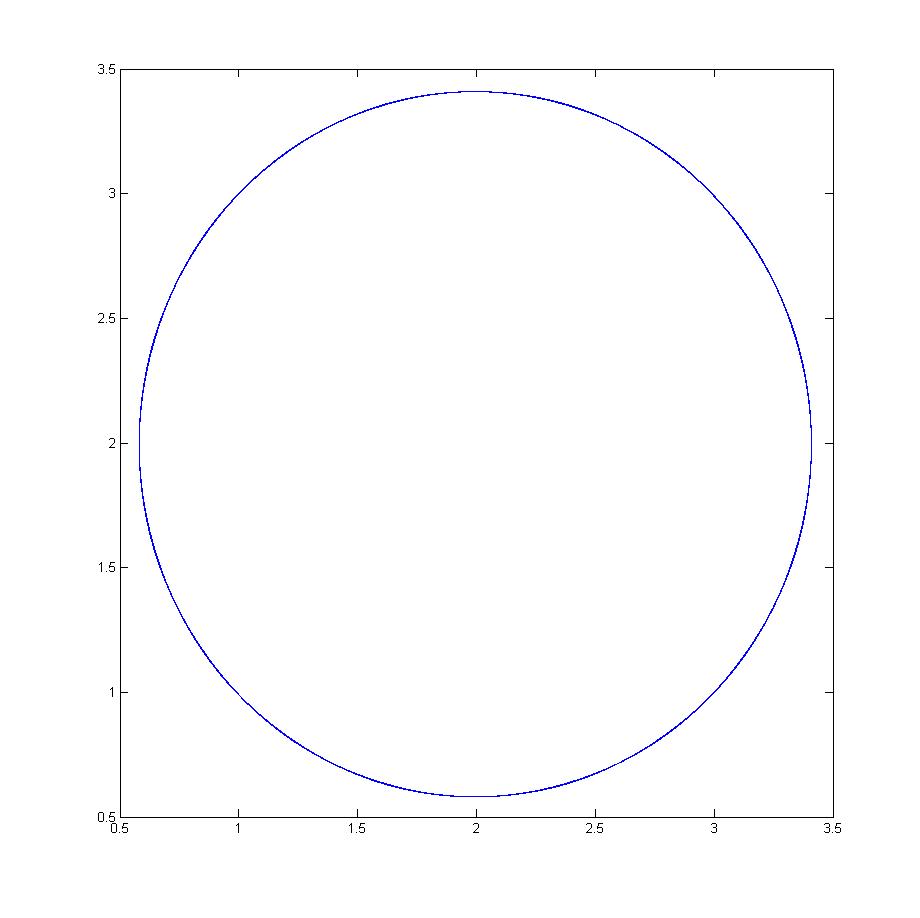
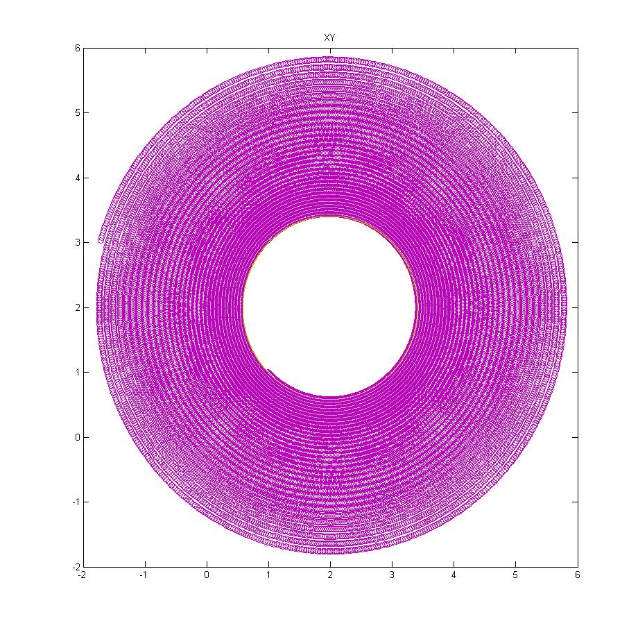
Figure 2. Orbits for the discrete nonholonomic equations of motion (left) and a standard numerical method (right) (initial conditions $x(0)=0.99$, $y(0)=1$, $x(1)=1$, $y(1)=0.99$ and $h=0.01$ after $20000$ steps).

4.6. Discrete Chaplygin systems

Now, we present the theory for a particular (but typical) example of discrete nonholonomic systems: discrete Chaplygin systems. This kind of systems was considered in the case of the pair groupoid in [10].

For any groupoid $\Gamma\rightrightarrows M$, the map $\chi:\Gamma\rightarrow M\times M$, $g\mapsto(\alpha(g),\beta(g))$ is a morphism over $M$ from $\Gamma$ to the pair groupoid $M\times M$ (usually called the anchor of $\Gamma$). The induced morphism of Lie algebroids is precisely the anchor $\rho:E_{\Gamma}\rightarrow TM$ of $E_{\Gamma}$ (the Lie algebroid of $\Gamma$).

Definition 4.2.

A discrete Chaplygin system on the groupoid $\Gamma$ is a discrete nonholonomic problem $(L_{d},{\mathcal{M}}_{c},{\mathcal{D}}_{c})$ such that

• $(L_{d},{\mathcal{M}}_{c},{\mathcal{D}}_{c})$ is a regular discrete nonholonomic Lagrangian system;

• $\chi_{{\mathcal{M}}_{c}}=\chi\circ i_{{\mathcal{M}}_{c}}:{\mathcal{M}}_{c}\longrightarrow M\times M$ is a diffeomorphism;

• $\rho\circ i_{{\mathcal{D}}_{c}}:{\mathcal{D}}_{c}\longrightarrow TM$ is an isomorphism of vector bundles.

Denote by $\tilde{L}_{d}:M\times M\longrightarrow\mathbb{R}$ the discrete Lagrangian defined by $\tilde{L}_{d}=L_{d}\circ i_{{\mathcal{M}}_{c}}\circ(\chi_{{\mathcal{M}}_{c}})^{-1}$.

In the following, we want to express the dynamics on $M\times M$, by finding relations between de dynamics defined by the nonholonomic system on $\Gamma$ and $M\times M$.

From our hypothesis, for any vector field $Y\in{\mathfrak{X}}(M)$ there exists a unique section $X\in\operatorname{Sec}(\tau_{{\mathcal{D}}_{c}})$ such that $\rho\circ i_{{\mathcal{D}}_{c}}\circ X=Y$.

Now, using (2.4), (2.5) and (2.6), it follows that

$$T_{g}\alpha(\overrightarrow{X}(g))=-Y(\alpha(g))\ \hbox{ and }\ T_{g}\beta(\overleftarrow{X}(g))=Y(\beta(g))$$

with some abuse of notation. In other words,

$${\mathcal{T}}_{g}\chi(X^{(1,0)}(g))=Y^{(1,0)}(\alpha(g),\beta(g))\ \hbox{ and }\ {\mathcal{T}}_{g}\chi(X^{(0,1)}(g))=Y^{(0,1)}(\alpha(g),\beta(g))$$

for $g\in{\mathcal{M}}_{c}$, where ${\mathcal{T}}\chi:{\mathcal{T}}^{\Gamma}\Gamma\cong V\beta\oplus_{\Gamma}V\alpha\to{\mathcal{T}}^{M\times M}(M\times M)\cong T(M\times M)$ is the prolongation of the morphism $\chi$ given by

$$({\mathcal{T}}_{g}\chi)(X_{g},Y_{g})=((T_{g}\alpha)(X_{g}),(T_{g}\beta)(Y_{g})),$$

for $g\in\Gamma$ and $(X_{g},Y_{g})\in{\mathcal{T}}^{\Gamma}_{g}\Gamma\cong V_{g}\beta\oplus V_{g}\alpha$.

Since $\chi_{{\mathcal{M}}_{c}}$ is a diffeomorphism, there exists a unique $X^{\prime}_{g}\in T_{g}{\mathcal{M}}_{c}$ (respectively, $\bar{X}^{\prime}_{g}\in T_{g}{\mathcal{M}}_{c}$) such that

$$({\mathcal{T}}_{g}\chi_{{\mathcal{M}}_{c}})(X^{\prime}_{g})=Y^{(1,0)}(\alpha(g),\beta(g))=(-Y(\alpha(g)),0_{\beta(g)})$$

(respectively, $({\mathcal{T}}_{g}\chi_{{\mathcal{M}}_{c}})(\bar{X}^{\prime}_{g})=Y^{(0,1)}(\alpha(g),\beta(g))=(0_{\alpha(g)},Y(\beta(g)))$) for all $g\in{\mathcal{M}}_{c}$.

Thus,

$$\begin{array}[]{l}X^{\prime}_{g}\in T_{g}{\mathcal{M}}_{c}\cap V_{g}\beta,\quad\overrightarrow{X}(g)-X^{\prime}_{g}=Z^{\prime}_{g}\in V_{g}\alpha\cap V_{g}\beta,\\ \bar{X}^{\prime}_{g}\in T_{g}{\mathcal{M}}_{c}\cap V_{g}\alpha,\quad\overleftarrow{X}(g)-\bar{X}^{\prime}_{g}=\bar{Z}^{\prime}_{g}\in V_{g}\alpha\cap V_{g}\beta,\end{array}$$

for all $g\in{\mathcal{M}}_{c}$.

Now, if $(g,h)\in\Gamma_{2}\cap({\mathcal{M}}_{c}\times{\mathcal{M}}_{c})$ then

$$\overleftarrow{X}(g)(L_{d})-\overrightarrow{X}(h)(L_{d}) = \bar{X}^{\prime}_{g}(L_{d})+\bar{Z}^{\prime}_{g}(L_{d})-{X}^{\prime}_{h}(L_{d})-Z^{\prime}_{h}(L_{d})$$

$$= \overleftarrow{Y}(\alpha(g),\beta(g))(\tilde{L}_{d})-\overrightarrow{Y}(\alpha(h),\beta(h))(\tilde{L}_{d})$$

$$+\bar{Z}^{\prime}_{g}(L_{d})-Z^{\prime}_{h}(L_{d}).$$

Therefore, if we use the following notation

$$\begin{array}[]{l}(\alpha(g),\beta(g))=(x,y),\qquad(\alpha(h),\beta(h))=(y,z)\\ F_{Y}^{+}(x,y)=-\bar{Z}^{\prime}_{\chi^{-1}_{{\mathcal{M}}_{c}}(x,y)}(L_{d}),\quad F_{Y}^{-}(y,z)=Z^{\prime}_{\chi^{-1}_{{\mathcal{M}}_{c}}(y,z)}(L_{d}),\end{array}$$

then

$$\overleftarrow{X}(g)(L_{d})-\overrightarrow{X}(h)(L_{d}) = \overleftarrow{Y}(x,y)(\tilde{L}_{d})-\overrightarrow{Y}(y,z)(\tilde{L}_{d})$$

$$-F_{Y}^{+}(x,y)+F_{Y}^{-}(y,z).$$

In conclusion, we have proved that $(g,h)$ is a solution of the discrete nonholonomic Euler-Lagrange equations for the system $(L_{d},{\mathcal{M}}_{c},{\mathcal{D}}_{c})$ if and only if $((x,y),(y,z))$ is a solution of the reduced equations

$$\overleftarrow{Y}(x,y)(\tilde{L}_{d})-\overrightarrow{Y}(y,z)(\tilde{L}_{d})=F_{Y}^{+}(x,y)-F_{Y}^{-}(y,z),\qquad Y\in\mathfrak{X}(M).$$

Note that the above equations are the standard forced discrete Euler-Lagrange equations (see [32]).

4.6.1. The discrete two wheeled planar mobile robot

We now consider a discrete version of the two-wheeled planar mobile robot [8, 9]. The position and orientation of the robot is determined, with respect a fixed cartesian reference, by an element $\Omega=(\theta,x,y)\in SE(2)$, that is, a matrix

$$\Omega=\left(\begin{array}[]{ccc}\cos\theta&-\sin\theta&x\\ \sin\theta&\cos\theta&y\\ 0&0&1\\ \end{array}\right).$$

Moreover, the different positions of the two wheels are described by elements $(\phi,\psi)\in\mathbb{T}^{2}$. Therefore, the configuration space is $SE(2)\times\mathbb{T}^{2}$. The system is subjected to three nonholonomic constraints: one constraint induced by the condition of no lateral sliding of the robot and the other two by the rolling conditions of both wheels.

It is well known that this system is $SE(2)$-invariant and then the system may be described as a nonholonomic system on the Lie algebroid $\mathfrak{se}(2)\times T\mathbb{T}^{2}\to\mathbb{T}^{2}$ (see [9]). In this case, the Lagrangian is

$$L = \frac{1}{2}\left(J\omega^{2}+m(v^{1})^{2}+m(v^{2})^{2}+2m_{0}l\omega v^{2}+J_{2}\dot{\phi}^{2}+J_{2}\dot{\psi}^{2}\right)$$

$$= \frac{1}{2}\operatorname{Tr}(\xi\mathbb{J}\xi^{T})+\frac{J_{2}}{2}\dot{\phi}^{2}+\frac{J_{2}}{2}\dot{\psi}^{2}$$

where

$$\xi=\omega\,e+v^{1}\,e_{1}+v^{2}\,e_{2}=\left(\begin{array}[]{ccc}0&-\omega&v^{1}\\ \omega&0&v^{2}\\ 0&0&0\end{array}\right)\qquad\hbox{and}\qquad\mathbb{J}=\left(\begin{array}[]{ccc}J/2&0&m_{0}l\\ 0&J/2&0\\ m_{0}l&0&m\end{array}\right)$$

Here, $m=m_{0}+2m_{1}$, where $m_{0}$ is the mass of the robot without the two wheels, $m_{1}$ the mass of each wheel, $J$ its the moment of inertia with respect to the vertical axis, $J_{2}$ the axial moments of inertia of the wheels and $l$ the distance between the center of mass of the robot and the intersection point of the horizontal symmetry axis of the robot and the horizontal line connecting the centers of the two wheels.

The nonholonomic constraints are

$$\begin{array}[]{rcl}v^{1}+\frac{R}{2}\dot{\phi}+\frac{R}{2}\dot{\psi}&=&0,\\ v^{2}&=&0,\\ \omega+\frac{R}{2c}\dot{\phi}-\frac{R}{2c}\dot{\psi}&=&0,\end{array}$$ (4.23)

determining a submanifold ${\mathcal{M}}$ of ${\mathfrak{s}e}(2)\times T\mathbb{T}^{2}$, where $R$ is the radius of the two wheels and $2c$ the lateral length of the robot.

In order to discretize the above nonholonomic system, we consider the Atiyah groupoid $\Gamma=SE(2)\times(\mathbb{T}^{2}\times\mathbb{T}^{2})\rightrightarrows\mathbb{T}^{2}$. The Lie algebroid of $SE(2)\times(\mathbb{T}^{2}\times\mathbb{T}^{2})\rightrightarrows\mathbb{T}^{2}$ is $T\mathbb{T}^{2}\times\mathfrak{se}(2)\to\mathbb{T}^{2}$. Then:

• The discrete Lagrangian $L_{d}:SE(2)\times(\mathbb{T}^{2}\times\mathbb{T}^{2})\rightarrow\mathbb{R}$ is given by:

  $$\begin{array}[]{rcl}L_{d}(\Omega_{k},\phi_{k},\psi_{k},\phi_{k+1},\psi_{k+1})&=&\frac{1}{2h^{2}}\hbox{Tr }((\Omega_{k}-I_{3\times 3})\mathbb{J}(\Omega_{k}-I_{3\times 3})^{T})\\ &&+\frac{J_{1}}{2}\frac{(\Delta\phi_{k})^{2}}{h^{2}}+\frac{J_{1}}{2}\frac{(\Delta\psi_{k})^{2}}{h^{2}},\end{array}$$

  where $I_{3\times 3}$ is the identity matrix, $\Delta\phi_{k}=\phi_{k+1}-\phi_{k}$, $\Delta\psi_{k}=\psi_{k+1}-\psi_{k}$ and

  $$\Omega_{k}=\left(\begin{array}[]{lll}\cos\theta_{k}&-\sin\theta_{k}&x_{k}\\ \sin\theta_{k}&\cos\theta_{k}&y_{k}\\ 0&0&1\end{array}\right).$$

  We obtain that

  $$L_{d} = \frac{1}{2h^{2}}\left(mx^{2}_{k}+my_{k}^{2}-2lm_{0}x_{k}(1-\cos\theta_{k})\right.$$

  $$\left.+2J(1-\cos\theta_{k})+2lm_{0}y_{k}\sin\theta_{k}\right)+\frac{1}{2}{J_{1}}\frac{(\Delta\phi_{k})^{2}}{h^{2}}+\frac{1}{2}J_{1}\frac{(\Delta\psi_{k})^{2}}{h^{2}}.$$

• The constraint vector subbundle of $\mathfrak{se}(2)\times T\mathbb{T}^{2}$ is generated by the sections:

  $$\left\{s_{1}=\frac{R}{2}e_{1}+\frac{R}{2c}e-\frac{\partial}{\partial\phi},s_{2}=\frac{R}{2}e_{1}-\frac{R}{2c}e-\frac{\partial}{\partial\psi}\right\}.$$

• The continuous constraints of the two-wheeled planar robot are written in matrix form (see 4.23):

  $$\xi=\left(\begin{array}[]{ccc}0&-\omega&v^{1}\\ \omega&0&v^{2}\\ 0&0&0\end{array}\right)=\left(\begin{array}[]{ccc}0&\frac{R}{2c}\dot{\phi}-\frac{R}{2c}\dot{\psi}&-\frac{R}{2}\dot{\phi}-\frac{R}{2}\dot{\psi}\\ -\frac{R}{2c}\dot{\phi}+\frac{R}{2c}\dot{\psi}&0&0\\ 0&0&0\end{array}\right)$$

  We discretize the previous constraints using the exponential on $SE(2)$ (see Section 4.3.2) and discretizing the velocities on the right hand side

  $$\Omega_{k}=\left(\begin{smallmatrix}\cos\left(\frac{R}{2c}\Delta{\phi}_{k}-\frac{R}{2c}\Delta{\psi}_{k}\right)&\sin\left(\frac{R}{2c}\Delta{\phi}_{k}-\frac{R}{2c}\Delta{\psi}_{k}\right)&-c\frac{\Delta{\phi}_{k}+\Delta{\psi}_{k}}{\Delta{\phi}_{k}-\Delta{\psi}_{k}}\sin\left(\frac{R}{2c}\Delta{\phi}_{k}-\frac{R}{2c}\Delta{\psi}_{k}\right)\\ -\sin\left(\frac{R}{2c}\Delta{\phi}_{k}-\frac{R}{2c}\Delta{\psi}_{k}\right)&\cos\left(\frac{R}{2c}\Delta{\phi}_{k}-\frac{R}{2c}\Delta{\psi}_{k}\right)&c\frac{\Delta{\phi}_{k}+\Delta{\psi}_{k}}{\Delta{\phi}_{k}-\Delta{\psi}_{k}}\left(1-\cos\left(\frac{R}{2c}\Delta{\phi}_{k}-\frac{R}{2c}\Delta{\psi}_{k}\right)\right)\\ 0&0&1\end{smallmatrix}\right)$$

  if $\Delta{\phi}_{k}\not=\Delta{\psi}_{k}$ and

  $$\Omega_{k}=\left(\begin{array}[]{ccc}1&0&-R\Delta{\phi}_{k}\\ 0&1&0\\ 0&0&1\end{array}\right)$$

  if $\Delta{\phi}_{k}=\Delta{\psi}_{k}$.

  Therefore, the constraint submanifold ${\mathcal{M}}_{c}$ is defined as

  $$\theta_{k} = -\frac{R}{2c}\Delta{\phi}_{k}+\frac{R}{2c}\Delta{\psi}_{k}$$ (4.24)

  $$x_{k} = -c\frac{\Delta{\phi}_{k}+\Delta{\psi}_{k}}{\Delta{\phi}_{k}-\Delta{\psi}_{k}}\sin\left(\frac{R}{2c}\Delta{\phi}_{k}-\frac{R}{2c}\Delta{\psi}_{k}\right)$$ (4.25)

  $$y_{k} = c\frac{\Delta{\phi}_{k}+\Delta{\psi}_{k}}{\Delta{\phi}_{k}-\Delta{\psi}_{k}}\left(1-\cos\left(\frac{R}{2c}\Delta{\phi}_{k}-\frac{R}{2c}\Delta{\psi}_{k}\right)\right)$$ (4.26)

  if $\Delta{\phi}_{k}\not=\Delta{\psi}_{k}$ and $\theta_{k}=0$, $x_{k}=-R\Delta{\phi}_{k}$ and $y_{k}=0$ if $\Delta{\phi}_{k}=\Delta{\psi}_{k}$.

We have that the discrete nonholonomic system $(L_{d},{\mathcal{M}}_{c},{\mathcal{D}}_{c})$ is reversible. Moreover, if $\epsilon_{\Gamma}:\mathbb{T}^{2}\to SE(2)\times(\mathbb{T}^{2}\times\mathbb{T}^{2})$ is the identity section of the Lie groupoid $\Gamma=SE(2)\times(\mathbb{T}^{2}\times\mathbb{T}^{2})$ then it is clear that

$$\epsilon_{\Gamma}(\mathbb{T}^{2})=\{I_{3\times 3}\}\times\Delta_{\mathbb{T}^{2}\times\mathbb{T}^{2}}\subseteq{\mathcal{M}}_{c}.$$

Here, $\Delta_{\mathbb{T}^{2}\times\mathbb{T}^{2}}$ is the diagonal in $\mathbb{T}^{2}\times\mathbb{T}^{2}$. In addition, the system $(L_{d},{\mathcal{M}}_{c},{\mathcal{D}}_{c})$ is regular in a neighborhood $U$ of the submanifold $\epsilon_{\Gamma}(\mathbb{T}^{2})=\{I_{3\times 3}\}\times\Delta_{\mathbb{T}^{2}\times\mathbb{T}^{2}}$ in ${\mathcal{M}}_{c}$. Note that

$$T_{(I_{3\times 3},\phi_{1},\psi_{1},\phi_{1},\psi_{1})}{\mathcal{M}}_{c}\cap E_{\Gamma}(\phi_{1},\psi_{1})={\mathcal{D}}_{c}(\phi_{1},\psi_{1}),$$

for $(\phi_{1},\psi_{1})\in\mathbb{T}^{2}$, where $E_{\Gamma}=\mathfrak{se}(2)\times T\mathbb{T}^{2}$ is the Lie algebroid of the Lie groupoid $\Gamma=SE(2)\times(\mathbb{T}^{2}\times\mathbb{T}^{2})$.

On the other hand, it is easy to show that the system $(L_{d},U,{\mathcal{D}}_{c})$ is a discrete Chaplygin system.

The reduced Lagrangian on $\mathbb{T}^{2}\times\mathbb{T}^{2}$ is

$$\tilde{L}_{d}=\left\{\begin{array}[]{l}\displaystyle\frac{1}{h^{2}}(mc^{2}(\frac{\Delta{\phi}_{k}+\Delta{\psi}_{k}}{\Delta{\phi}_{k}-\Delta{\psi}_{k}})^{2}(1-\cos(\frac{R}{2c}\Delta{\phi}_{k}-\frac{R}{2c}\Delta{\psi}_{k}))\\ \displaystyle+J(1-\cos(\frac{R}{2c}\Delta{\phi}_{k}-\frac{R}{2c}\Delta{\psi}_{k})))+\frac{1}{2}J_{1}\frac{(\Delta\phi_{k})^{2}}{h^{2}}+\frac{1}{2}J_{1}\frac{(\Delta\psi_{k})^{2}}{h^{2}}\quad\hbox{if}\quad\Delta{\phi}_{k}\not=\Delta{\psi}_{k}\\[15.0pt] \displaystyle(J_{1}+\frac{mR^{2}}{2})\frac{(\Delta\phi_{k})^{2}}{h^{2}},\quad\hbox{if}\quad\Delta{\phi}_{k}=\Delta{\psi}_{k}\end{array}\right.$$

The discrete nonholonomic equations are:

$$\overleftarrow{s_{1}}\big{|}_{(\Omega_{1},\phi_{1},\psi_{1},\phi_{2},\psi_{2})}(L_{d})-\overrightarrow{s_{1}}\big{|}_{(\Omega_{2},\phi_{2},\psi_{2},\phi_{3},\psi_{3})}(L_{d}) = 0$$

$$\overleftarrow{s_{2}}\big{|}_{(\Omega_{1},\phi_{1},\psi_{1},\phi_{2},\psi_{2})}(L_{d})-\overrightarrow{s_{2}}\big{|}_{(\Omega_{2}\phi_{2},\psi_{2},\phi_{3},\psi_{3})}(L_{d}) = 0$$

These equations in coordinates are:

$$2J_{1}(\phi_{3}-2\phi_{2}+\phi_{1})=lRm_{0}(\cos\theta_{2}+\cos\theta_{1})+\frac{JR}{c}(\sin\theta_{2}-\sin\theta_{1})$$

$$-\frac{R\cos\theta_{1}}{c}(lm_{0}y_{1}+cmx_{1})+\frac{R\sin\theta_{1}}{c}(lm_{0}x_{1}-cmy_{1})$$

$$+\frac{R}{c}(cmx_{2}+lm_{0}(y_{2}-2c))$$ (4.27)

$$2J_{1}(\psi_{3}-2\psi_{2}+\psi_{1})=lRm_{0}(\cos\theta_{2}+\cos\theta_{1})-\frac{JR}{c}(\sin\theta_{2}-\sin\theta_{1})$$

$$+\frac{R\cos\theta_{1}}{c}(lm_{0}y_{1}-cmx_{1})-\frac{R\sin\theta_{1}}{c}(lm_{0}x_{1}+cmy_{1})$$

$$+\frac{R}{c}(cmx_{2}-lm_{0}(y_{2}+2c))$$ (4.28)

Substituting constraints (4.24), (4.25) and (4.26) in Equations (4.27) and (4.28) we obtain a set of equations of the type $0=f_{1}(\phi_{1},\phi_{2},\phi_{3},\psi_{1},\psi_{2},\psi_{3})$ and $0=f_{1}(\phi_{1},\phi_{2},\phi_{3},\psi_{1},\psi_{2},\psi_{3})$ which are the reduced equations of the Chaplygin system.

5. Conclusions and Future Work

In this paper we have elucidated the geometrical framework for nonholonomic discrete Mechanics on Lie groupoids. We have proposed discrete nonholonomic equations that are general enough to produce practical integrators for continuous nonholonomic systems (reduced or not). The geometric properties related with these equations have been completely studied and the applicability of these developments has been stated in several interesting examples.

Of course, much work remains to be done to clarify the nature of discrete nonholonomic mechanics. Many of this future work was stated in [36] and, in particular, we emphasize:

• a complete backward error analysis which explain the very good energy behavior showed in examples or the preservation of a discrete energy (see [14]);

• related with the previous question, the construction of a discrete exact model for a continuous nonholonomic system (see [17, 32, 36]);

• to study discrete nonholonomic systems which preserve a volume form on the constraint surface mimicking the continuous case (see, for instance, [13, 46] for this last case);

• to analyze the discrete hamiltonian framework and the construction of integrators depending on different discretizations;

• and the construction of a discrete nonholonomic connection in the case of Atiyah groupoids (see [21, 27]).

Related with some of the previous questions, in the conclusions of the paper of R. McLachlan and M. Perlmutter [36], the authors raise the question of the possibility of the definition of generalized constraint forces dependent on all the points $q_{k-1}$, $q_{k}$ and $q_{k+1}$ (instead of just $q_{k}$) for the case of the pair groupoid. We think that the discrete nonholonomic Euler-Lagrange equations can be generalized to consider this case of general constraint forces that, moreover, are closest to the continuous model (see [25, 36]).

References

-
[1]
Arnold VI
Mathematical Methods of Classical Mechanics Graduate Text in Mathematics 60, Springer-Verlag New York, 1978. -
[2]
Bates L and Śniatycki J
Nonholonomic reduction Rep. on Math. Phys. 32 (1992) (1) 99–115. -
[3]
Bloch AM
Nonholonomic Mechanics and Control Interdisciplinary Applied Mathematics Series 24, Springer-Verlag New-York, 2003. -
[4]
Bloch AM, Krishnaprasad PS, Marsden JE and
Murray RM
Nonholonomic mechanical systems with symmetry Arch. Rational Mech. Anal. 136 (1996) 21–99. -
[5]
Bobenko AI and Suris YB
Discrete Lagrangian reduction, discrete Euler-Poincaré equations, and semidirect products Lett. Math. Phys. 49 (1999), 79–93. -
[6]
Bobenko AI and Suris YB
Discrete time Lagrangian mechanics on Lie groups, with an application to the Lagrange top Comm. Math. Phys. 204 (1999) 147–188. -
[7]
Coste A, Dazord P and Weinstein A
Grupoïdes symplectiques Pub. Dép. Math. Lyon, 2/A (1987), 1–62. -
[8]
Cortés J
Geometric, control and numerical aspects of nonholonomic systems Lecture Notes in Mathematics, 1793 (2002), Springer-Verlag. -
[9]
Cortés J, de León M, Marrero JC and
Martínez E
Nonholonomic Lagrangian systems on Lie algebroids Preprint math-ph/0512003. -
[10]
Cortés J and Martínez S
Nonholonomic integrators Nonlinearity 14 (2001), 1365–1392. -
[11]
Cortés J and Martínez E
Mechanical control systems on Lie algebroids IMA J. Math. Control. Inform. 21 (2004), 457–492. -
[12]
Fedorov YN
A Discretization of the Nonholonomic Chaplygin Sphere Problem SIGMA 3 (2007), 044, 15 pages. -
[13]
Fedorov YN and Jovanovic B
Nonholonomic LR systems as generalized Chaplygin systems with an invariant measure and flows on homogeneous spaces J. Nonlinear Sci. 14 (4) (2004), 341–381. -
[14]
Fedorov YN and Zenkov DV