Stochastic fluctuations in metabolic pathways

Abstract

Fluctuations in the abundance of molecules in the living cell may affect its growth and well being. For regulatory molecules (e.g., signaling proteins or transcription factors), fluctuations in their expression can affect the levels of downstream targets in a network. Here, we develop an analytic framework to investigate the phenomenon of noise correlation in molecular networks. Specifically, we focus on the metabolic network, which is highly inter-linked, and noise properties may constrain its structure and function. Motivated by the analogy between the dynamics of a linear metabolic pathway and that of the exactly soluable linear queueing network or, alternatively, a mass transfer system, we derive a plethora of results concerning fluctuations in the abundance of intermediate metabolites in various common motifs of the metabolic network. For all but one case examined, we find the steady-state fluctuation in different nodes of the pathways to be effectively uncorrelated. Consequently, fluctuations in enzyme levels only affect local properties and do not propagate elsewhere into metabolic networks, and intermediate metabolites can be freely shared by different reactions. Our approach may be applicable to study metabolic networks with more complex topologies, or protein signaling networks which are governed by similar biochemical reactions. Possible implications for bioinformatic analysis of metabolimic data are discussed.

Due to the limited number of molecules for typical molecular species in microbial cells, random fluctuations in molecular networks are common place and may play important roles in vital cellular processes. For example, noise in sensory signals can result in pattern formation and collective dynamics [1], and noise in signaling pathways can lead to cell-to-cell variability [2]. Also, stochasticity in gene expression has implications on cellular regulation [3, 4] and may lead to phenotypic diversity [5, 6], while fluctuations in the levels of (toxic) metabolic intermediates may reduce metabolic efficiency [7] and impede cell growth.

In the past several years, a great deal of experimental and theoretical efforts have focused on the stochastic expression of individual genes, at both the translational and transcriptional levels [8, 9, 10]. The effect of stochasticity on networks has been studied in the context of small, ultra-sensitivie genetic circuits, where noise at a circuit node (i.e., a gene) was shown to either attenuate or amplify output noise in the steady state [11, 12]. This phenomenon — termed ‘noise propagation’ — make the steady-state fluctuations at one node of a gene network dependent in a complex manner on fluctuations at other nodes, making it difficult for the cell to control the noisiness of individual genes of interest [13]. Several key questions which arise from these studies of genetic noise include (i) whether stochastic gene expression could further propagate into signaling and metabolic networks through fluctuations in the levels of key proteins controlling those circuits, and (ii) whether noise propagation occurs also in those circuits.

Recently, a number of approximate analytical methods have been applied to analyze small genetic and signaling circuits; these include the independent noise approximation [14, 15, 16], the linear noise approximation [14, 17], and the self-consistent field approximation [18]. Due perhaps to the different approximation schemes used, conflicting conclusions have been obtained regarding the extent of noise propagation in various networks (see, e.g., [17].) Moreover, it is difficult to extend these studies to investigate the dependences of noise correlations on network properties, e.g., circuit topology, nature of feedback, catalytic properties of the nodes, and the parameter dependences (e.g., the phase diagram). It is of course also difficult to elucidate these dependences using numerical simulations alone, due to the very large degrees of freedoms involved for a network with even a modest number of nodes and links.

In this study, we describe an analytic approach to characterize the probability distribution for all nodes of a class of molecular networks in the steady state. Specifically, we apply the method to analyze fluctuations and their correlations in metabolite concentrations for various core motifs of the metabolic network. The metabolic network consists of nodes which are the metabolites, linked to each other by enzymatic reactions that convert one metabolite to another. The predominant motif in the metabolic network is a linear array of nodes linked in a given direction (the directed pathway), which are connected to each other via converging pathways and diverging branch points [19]. The activities of the key enzymes are regulated allosterically by metabolites from other parts of the network, while the levels of many enzymes are controlled transcriptionally and are hence subject to deterministic as well as stochastic variations in their expressions [20]. To understand the control of metabolic network, it is important to know how changes in one node of the network affect properties elsewhere.

Applying our analysis to directed linear metabolic pathways, we predict that the distribution of molecule number of the metabolites at intermediate nodes to be statistically independent in the steady state, i.e., the noise does not propagate. Moreover, given the properties of the enzymes in the pathway and the input flux, we provide a recipe which specifies the exact metabolite distribution function at each node. We then show that the method can be extended to linear pathways with reversible links, with feedback control, to cyclic and certain converging pathways, and even to pathways in which flux conservation is violated (e.g., when metabolites leak out of the cell). We find that in these cases correlations between nodes are negligable or vanish completely, although nontrivial fluctuation and correlation do dominate for a special type of converging pathways. Our results suggest that for vast parts of the metabolic network, different pathways can be coupled to each other without generating complex correlations, so that properties of one node (e.g., enzyme level) can be changed over a broad range without affecting behaviors at other nodes. We expect that the realization of this remarkable property will shape our understanding of the operation of the metabolic network, its control, as well as its evolution. For example, our results suggest that correlations between steady-state fluctuations in different metabolites bare no information on the network structure. In contrast, temporal propagation of the response to an external perturbation should capture - at least locally - the morphology of the network. Thus, the topology of the metabolic network should be studied during transient periods of relaxation towards a steady-state, and not at steady-state.

Our method is motivated by the analogy between the dynamics of biochemical reactions in metabolic pathways and that of the exactly solvable queueing systems [46] or, alternatively, as mass transfer systems [22, 47]. Our approach may be applicable also to analyzing fluctuations in signaling networks, due to the close analogy between the molecular processes underlying the metabolic and signaling networks. To make our approach accessible to a broad class of circuit modelers and bioengineers who may not be familiar with nonequilibrium statistical mechanics, we will present in the main text only the mathematical results supported by stochastic simulations, and defer derivations and illustrative calculations to the Supporting Materials. While our analysis is general, all examples are taken from amino-acid biosynthesis pathways in E. Coli [24].

1 Individual Nodes

1.1 A molecular Michaelis-Menton model

In order to set up the grounds for analyzing a reaction pathway and to introduce our notation, we start by analyzing fluctuations in a single metabolic reaction catalyzed by an enzyme.

Recent advances in experimental techniques have made it possible to track the enzymatic turnover of a substrate to product at the single-molecule level [26, 27], and to study instantaneous metabolite concentration in the living cell [28]. To describe this fluctuation mathematically, we model the cell as a reaction vessel of volume $V$, containing $m$ substrate molecules ($S$) and $N_{E}$ enzymes ($E$). A single molecule of $S$ can bind to a single enzyme $E$ with rate $k_{+}$ per volume, and form a complex, $SE$. This complex, in turn, can unbind (at rate $k_{-}$) or convert $S$ into a product form, $P$, at rate $k_{2}$. This set of reactions is summarized by

$$S+E\mathop{\leftrightarrows}^{k_{+}}_{k_{-}}SE\mathop{\rightarrow}^{k_{2}}P+E\;.$$ (1)

Analyzing these reactions within a mass-action framework — keeping the substrate concentration fixed, and assuming fast equilibration between the substrate and the enzymes $(k_{\pm}\gg k_{2})$ — leads to the Michaelis-Menten (MM) relation between the macroscopic flux $c$ and the substrate concentration $[S]=m/V$ :

$$c=v_{\max}[S]/([S]+K_{M})\;,$$ (2)

where $K_{M}=k_{-}/k_{+}$ is the dissociation constant of the substrate and the enzyme, and $v_{\max}=k_{2}[E]$ is the maximal flux, with $[E]=N_{E}/V$ being the total enzyme concentration.

Our main interest is in noise properties, resulting from the discreteness of molecules. We therefore need to track individual turnover events. These are described by the turnover rate $w_{m}$, defined as the inverse of the mean waiting time per volume between the (uncorrelated) synthesis of one product molecule to the next. Assuming again fast equilibration between the substrate and the enzymes, the probability of having $N_{SE}$ complexes given $m$ substrate molecules and $N_{E}$ enzymes is simply given by the Boltzmann distribution,

$$p(N_{SE}|m,N_{E})=\frac{K^{-N_{SE}}}{Z_{m,N_{E}}}\frac{m!N_{E}!}{N_{SE}!(m-N_{SE})!(N_{E}-N_{SE})!}\;$$ (3)

for $N_{SE}<N_{E}$ and $m$. Here $K^{-1}=Vk_{+}/k_{-}$ is the Boltzmann factor associated with the formation of an SE complex, and the $Z_{m,N_{E}}$ takes care of normalization (i.e., chosen such that $\sum_{N_{SE}}\,p(N_{SE}|m,N_{E})=1$.) Under this condition, the turnover rate $w_{m}=\frac{k_{2}}{V}\sum{N_{SE}}\cdot p(N_{SE}|m,N_{E})$ is given approximately by

$$w_{m}=v_{\max}\frac{m}{m+(K+N_{E}-1)}+{\cal O}(K^{-3})\;,$$ (4)

with $v_{\max}=k_{2}N_{E}/V$; see Supp. Mat. We note that for a single enzyme ($N_{E}=1$), one has $w_{m}=v_{\max}{m}/{(m+K)}$, which was derived and verified experimentally [27, 29].

1.2 Probability distribution of a single node

In a metabolic pathway, the number of substrate molecules is not kept fixed; rather, these molecules are synthesized or imported from the environment, and at the same time turned over into products. We consider the influx of substrate molecules to be a Poisson process with rate $c$. These molecules are turned into product molecules with rate $w_{m}$ given by Eq. ( 4 ). The number of substrate molecules is now fluctuating, and one can ask what is the probability $\pi(m)$ of finding $m$ substrate molecules at the steady-state. This probability can be found by solving the steady-state Master equation for this process (see Supp. Mat.), yielding

$$\pi(m)={m+K+(N_{E}-1)\choose m}(1-z)^{K+N_{E}}z^{m}\;,$$ (5)

where $z={c}/v_{\max}$ [31]. The form of this distribution is plotted in supporting figure 1 (solid black line). As expected, a steady state exists only when ${c}\leq v_{\max}$. Denoting the steady-state average by angular brackets, i.e., $\langle x_{m}\rangle\equiv\sum_{m}x_{m}\,\pi(m)$, the condition that the incoming flux equals the outgoing flux is written as

$$c=\langle w_{m}\rangle=v_{\max}\frac{s}{s+(K+N_{E})}\;,$$ (6)

where $s\equiv\langle m\rangle$.

Comparing this microscopically-derived flux-density relation with the MM relation ( 2 ) using the obvious correspondence $[S]=s/V$, we see that the two are equivalent with $K_{M}=(K+N_{E})/V$. Note that this microscopically-derived form of MM constant is different by the amount $[E]$ from the commonly used (but approximate form) $K_{M}=K/V$, derived from mass-action. However, for typical metabolic reactions, $K_{M}\sim 10-1000\,\mu M$ [24] while $[E]$ is not more than 1000 molecules in a bacterium cell ($\sim 1\mu M$); so the numerical values of the two expressions may not be very different.

We will characterize the variation of substrate concentration in the steady-state by the noise index

$$\eta_{s}^{2}\equiv\frac{\sigma_{s}^{2}}{s^{2}}=\frac{v_{\max}}{c\cdot(K+N_{E})}\;,$$ (7)

where $\sigma_{s}^{2}$ is the variance of the distribution $\pi(m)$. Since $c\leq v_{\max}$ and increases with $s$ towards $1$ (see Eq. 6),  $\eta_{s}$ decreases with the average occupancy $s$ as expected. It is bound from below by $1/\sqrt{K+N_{E}}$, which can easily be several percent. Generally, large noise is obtained when the reaction is catalyzed by a samll number of high-affinity enzymes (i.e., for low $K$ and $N_{E}$).

2 Linear pathways

2.1 Directed pathways

We now turn to a directed metabolic pathway, where an incoming flux of substrate molecules is converted, through a series of enzymatic reactions, into a product flux [19]. Typically, such a pathway involves the order of 10 reactions, each takes as precursor the product of the preceding reaction, and frequently involves an additional side-reactant (such as a water molecule or ATP) that is abundant in the cell (and whose fluctuations can be neglected). As a concrete example, we show in figure 1(a) the tryptophan biosynthesis pathway of E. Coli [24], where an incoming flux of chorismate is converted through 6 directed reactions into an outgoing flux of tryptophan, making use of several side-reactants. Our description of a linear pathway includes an incoming flux $c$ of substrates of type $S_{1}$ along with a set of reactions that convert substrate type $S_{i}$ to $S_{i+1}$ by enzyme $E_{i}$ (see figure 1(b)) with rate $w^{(i)}_{m_{i}}=v_{i}m_{i}/(m_{i}+K_{i}-1)$ according to Eq. ( 4 ). We denote the number of molecules of intermediate $S_{i}$ by $m_{i}$, with $m_{1}$ for the substrate and $m_{L}$ for the end-product. The superscript $(i)$ indicates explicitly that the parameters $v_{i}=k_{2}^{(i)}N_{E}^{(i)}/V$ and $K_{i}=(K^{(i)}+N_{E}^{(i)})$ describing the enzymatic reaction $S_{i}\to S_{i+1}$ are expected to be different for different reactions.

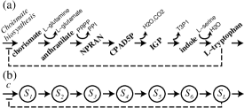
Figure 1: Linear biosynthesis pathway. (a) Tryptophan biosynthesis pathway in E. Coli. (b) Model for a directed pathway. Dashed lines depict end-product inhibition. Abbreviations: CPAD5P, 1-O-Carboxyphenylamino 1-deoxyribulose-5-phosphate; NPRAN, N-5-phosphoribosyl-anthranilate; IGP, Indole glycerol phosphate; PPI, Pyrophosphate; PRPP, 5-Phosphoribosyl-1-pyrophosphate; T3P1, Glyceraldehyde 3-phosphate.

The steady-state of the pathway is fully described by the joint probability distribution $\pi(m_{1},m_{2},\ldots,m_{L})$ of having $m_{i}$ molecules of intermediate substrate type $S_{i}$. Surprisingly, this steady-state distribution is given exactly by a product measure,

$$\pi(m_{1},m_{2},\ldots,m_{L})=\prod_{i=1}^{L}\pi_{i}(m_{i})\;,$$ (8)

where $\pi_{i}(m)$ is as given in Eq. ( 5 ) (with $K+N_{E}$ replaced by $K_{i}$ and $z$ by $z_{i}={c}/{v_{i}}$), as we show in Supp. Mat. This result indicates that in the steady state, the number of molecules of one intermediate is statistically independent of the number of molecules of any other substrate. The result has been derived previously in the context of queueing networks [46], and of mass-transport systems [47]. Either may serve as a useful analogy for a metabolic pathway.

Since the different metabolites in a pathway are statistically decoupled in the steady state, the mean $s_{i}=\langle m_{i}\rangle$ and the noise index $\eta_{s_{i}}^{2}=c^{-1}v_{i}/K_{i}$ can be determined by Eq. ( 7 ) individually for each node of the pathway. It is an interesting consequence of the decoupling property of this model that both the mean concentration of each substrate and the fluctuations depend only on the properties of the enzyme immediately downstream. While the steady-state flux $c$ is a constant throughout the pathway, the parameters $v_{i}$ and $K_{i}$ can be set separately for each reaction by the copy-number and kinetic properties of the enzymes (provided that $c<v_{i}$). Hence, for example, in a case where a specific intermediate may be toxic, tuning the enzyme properties may serve to decrease fluctuations in its concentration, at the price of a larger mean. To illustrate the decorrelation between different metabolites, we examine the response of steady-state fluctuations to a 5-fold increase in the enzyme level $[E_{1}]$. Typical time scale for changes in enzyme level much exceeds those of the enzymatic reactions. Hence, the enzyme level changes may be considered as quasi-steady state. In figure 2(a) we plot the noise indices of the different metabolites. While noise in the first node is significantly reduced upon a 5-fold increase in $[E_{1}]$, fluctuations at the other nodes are not affected at all.

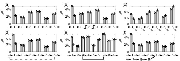
Figure 2: Noise in metabolite molecular number ($\eta_{s}=\sigma_{s}/s$) for different pathways. Monte-Carlo simulations (bars) are compared with the analytic prediction (symbols) obtained by assuming decorrelation for different nodes of the pathways. The structure of each pathway is depicted under each panel. Parameter values were chosen randomly such that $10^{3}<K_{i}<10^{4}$ and $c<v_{i}<10c$. SImilar decorrelation was obtained for $100$ different random choices of parameters, and for $100$ different sets with $K_{i}$ 10-fold smaller (data not shown). The effect on the different metabolites of a change in the velocity of the first reaction, $v_{1}=1.1c$ (dark gray)$\to 5c$ (light gray), is demonstrated. Similar results are obtained for changes in $K_{1}$ (data not shown.) (a) Directed pathway. Here the decorrelation property is exact. (b) Directed pathway with two reversible reactions. For these reactions, $v^{+}_{3,4}=8.4,6.9c;v^{-}_{3,4}=1.6,3.7,c;K_{3,4}^{+}=2500,8000$ and $K_{3,4}^{-}=7700,3700$. (c) Linear dilution of metabolites. Here $\beta/c=1/100$. (d) End-product inhibition,where the influx rate is given by $\alpha={c_{0}}\left[{1+(m_{L}/K_{I})}\right]^{-1}$ with $K_{I}=1000$. (e) Diverging pathways. Here metabolite $4$ is being processed by two enzymes (with different affinities, $K^{\mathtt{I}}=810,K^{\mathtt{II}}=370$) into metabolites $5$ and $7$, resp. (f) Converging pathways. Here two independent 3-reaction pathways , with fluxes $c$ and $c^{\prime}=c/2$, produce the same product, $S_{4}$.

2.2 Reversible reactions

The simple form of the steady-state distribution ( 8 ) for the directed pathways may serve as a starting point to obtain additional results for metabolic networks with more elaborate features. We demonstrate such applications of the method by some examples below. In many pathways, some of the reactions are in fact reversible. Thus, a metabolite $S_{i}$ may be converted to metabolite $S_{i+1}$ with rate $v_{\rm max}^{+}m_{i}/(m_{i}+K_{i}^{+})$ or to substrate $S_{i-1}$ with rate $v_{\rm max}^{-}m_{i}/(m_{i}+K_{i}^{-})$. One can show — in a way similar to Ref. [47] — that the decoupling property ( 5 ) holds exactly only if the ratio of the two rates is a constant independent of $m_{i}$, i.e. when $K_{i}^{+}=K_{i}^{-}$. In this case the steady state probability is still given by ( 5 ), with the local currents obeying

$$v_{i}^{+}z_{i}-v_{i+1}^{-}z_{i+1}=c\,.$$ (9)

This is nothing but the simple fact that the overall flux is the difference between the local current in the direction of the pathway and that in the opposite direction.

In general, of course, $K_{i}^{+}\neq K_{i}^{-}$. However, we expect the distribution to be given approximately by the product measure in the following situations: (a) $K_{i}^{+}\simeq K_{i}^{-}$; (b) the two reactions are in the zeroth-order regime, $s\gg K_{i}^{\pm}$ ; (c) the two reactions are in the linear regime, $s\ll K_{i}^{\pm}$. In the latter case Eq. ( 9 ) is replaced by $\frac{v_{i}^{+}}{K_{i}^{+}}z_{i}-\frac{v_{i+1}^{-}}{K_{i+1}^{-}}z_{k+1}=c\,.$ Taken together, it is only for a narrow region (i.e., $s_{i}\sim K_{i}$) where the product measure may not be applicable. This prediction is tested numerically, again by comparing two pathways (now containing reversible reactions) with 5-fold difference in the level of the first enzyme. From figure2(b), we see again that the difference in noise indices exist only in the first node, and the computed value of the noise index at each node is in excellent agreement with predictions based on the product measure (symbols). SImilar decorrelation was obtained for $100$ different random choices of parameters, and for $100$ different sets with $K_{i}$ 10-fold smaller (data not shown).

2.3 Dilution of intermediates

In the description so far, we have ignored possible catabolism of intermediates or dilution due to growth. This makes the flux a conserved quantity throughout the pathway, and is the basis of the flux-balance analysis [32]. One can generalize our framework for the case where flux is not conserved, by allowing particles to be degraded with rate $u_{m}$. Suppose, for example, that on top of the enzymatic reaction a substrate is subjected to an effective linear degradation, $u_{m}=\beta m$. This includes the effect of dilution due to growth, in which case $\beta=\ln(2)/$(mean cell division time), and the effect of leakage out of the cell. As before, we first consider the dynamics at a single node, where the metabolite is randomly produced (or transported) at a rate $c_{0}$. It is straightforward to generalize the Master equation for the microscopic process to include $u_{m}$, and solve it in the same way. With $w_{m}$ as before, the steady state distribution of the substrate pool size is then found to be

$$\pi(m)=\frac{1}{Z}{m+K-1\choose m}\frac{(c_{0}/\beta)^{m}}{(v/\beta+K)_{m}}\;,$$ (10)

where $(a)_{m}\equiv a(a+1)\cdots(a+m-1)$. This form of $\pi(m)$ allows one to easily calculate moments of the molecule number from the partition function $Z$ as in equilibrium statistical mechanics, e.g. $s=\langle m\rangle=c_{0}dZ/dc_{0}$, and thence the outgoing flux, $c=c_{0}-\beta s$. Using the fact that $Z$ can be written explicitly in terms of hypergeometric functions, we find that the noise index grows with $\beta$ as $\eta_{s}^{2}\simeq v/(Kc_{0})+\beta/c_{0}$. The distribution function is given in supporting figure 1 for several values of $\beta$.

Generalizing the above to a directed pathway, we allow for $\beta$, as well as for $v_{\max}$ and $K$, to be $i$-dependent. The decoupling property ( 8 ) does not generally hold in the non-conserving case [33]. However, in this case the stationary distribution still seems to be well approximated by a product of the single-metabolite functions $\pi_{i}(m)$ of the form ( 10 ), with $c_{0}/\beta\to c_{i-1}/\beta_{i}$. This is supported again by the excellent agreement between noise indices obtained by numerical simulations and analytic calculations using the product measure Ansatz, for linear pathways with dilution of intermediates; see figure 2(c). In this case, change in the level of the first enzyme does ”propagate” to the downstream nodes. But this is not a “noise propagation” effect, as the mean fluxes $\langle c_{i}\rangle$ at the different nodes are already affected. (To illustrate the effect of leakage, the simulation used parameters that corresponded to a huge leakage current which is $20\%$ of the flux. This is substantially larger than typical leakage encountered, say due to growth-mediated dilution, and we do not expect propagation effects due to leakage to be significant in practice.)

3 Interacting pathways

The metabolic network in a cell is composed of pathways of different topologies. While linear pathways are abundant, one can also find circular pathways (such as the TCA cycle), converging pathways and diverging ones. Many of these can be thought of as a composition of interacting linear pathways. Another layer of interaction is imposed on the system due to the allosteric regulation of enzyme activity by intermediate metabolites or end products. To what extent can our results for a linear pathway be applied to these more complex networks? Below we address this question for a few of the frequently encountered cases. To simplify the analysis, we will consider only directed pathways and suppress the dilution/leakage effect.

3.1 Cyclic pathways

We first address the cyclic pathway, in which the metabolite $S_{L}$ is converted into $S_{1}$ by the enzyme $E_{L}$. Borrowing a celebrated result for queueing networks [34] and mass transfer models [35], we note that the decoupling property ( 8 ) described above for the linear directed pathway also holds exactly even for the cyclic pathways. This result is surprising mainly because the Poissonian nature of the “incoming” flux assumed in the analysis so far is lost, replaced in this case by a complex expression, e.g., $w^{(L)}_{m_{L}}\cdot\pi_{L}(m_{L})$.

In an isolated cycle the total concentration of the metabolites, $s_{\rm tot}$ – and not the flux – is predetermined. In this case, the flux $c$ is give by the solution to the equation

$$s_{\rm tot}=\sum_{i=1}^{L}s_{i}(c)=\sum_{i=1}^{L}\frac{cK_{i}}{v_{i}-c}\;.$$ (11)

Note that this equation can always be satisfied by some positive $c$ that is smaller than all $v_{i}$’s. In a cycle that is coupled to other branches of the network, flux may be governed by metabolites going into the cycle or taken from it. In this case, flux balance analysis will enable determination of the variables $z_{i}$ which specify the probability distribution ( 5 ).

3.2 End-product inhibition

Many biosynthesis pathways couple between supply and demand by a negative feedback [24, 19], where the end-product inhibits the first reaction in the pathway or the transport of its precursor; see, e.g., the dashed lines in figure 1. In this way, flux is reduced when the end-product builds up. In branched pathways this may be done by regulating an enzyme immediately downstream from the branch-point, directing some of the flux towards another pathway.

To study the effect of end-product inhibition, we consider inhibition of the inflow into the pathway. Specifically, we model the probability at which substrate molecules arrive at the pathway by a stochastic process with exponentially-distributed waiting time, characterized by the rate $\alpha(m_{L})={c_{0}}\left[{1+(m_{L}/K_{I})^{h}}\right]^{-1}$, where $c_{0}$ is the maximal influx (determined by availability of the substrate either in the medium or in the cytoplasm), $m_{L}$ is the number of molecules of the end-product ($S_{L}$), $K_{I}$ is the dissociation constant of the interaction between the first enzyme $E_{0}$ and $S_{L}$, and $h$ is a Hill coefficient describing the cooperativity of interaction between $E_{0}$ and $S_{L}$. Because $m_{L}$ is a stochastic variable itself, the incoming flux is described by a nontrivial stochastic process which is manifestly non-Poissonian.

The steady-state flux is now

$$c=\langle\alpha(m_{L})\rangle=c_{0}\cdot\left\langle\left[1+(m_{L}/K_{I})^{h}\right]^{-1}\right\rangle\;.$$ (12)

This is an implicit equation for the flux $c$, which also appears in the right-hand side of the equation through the distribution $\pi(m_{1},...,m_{L})$.

By drawing an analogy between feedback-regulated pathway and a cyclic pathway, we conjecture that metabolites in the former should be effectively uncorrelated. The quality of this approximation is expected to become better in cases where the ration between the influx rate $\alpha(m_{L})$ and the outflux rate $w_{m_{L}}$ is typically $m_{L}$ idependent. Under this assumption, we approximate the distribution function by the product measure ( 8 ), with the form of the single node distributions given by ( 5 ). Note that the conserved flux then depends on the properties of the enzyme processing the last reaction, and in general should be influenced by the fluctuations in the controlling metabolite. In this sense, these fluctuations propagate throughout the pathway at the level of the mean flux. This should be expected from any node characterized by a high control coefficient [7].

Using this approximate form, Eq. ( 12 ) can be solved self-consistently to yield $c(c_{0})$, as is shown explicitly in Supp. Mat. for $h=1$. The solution obtained is found to be in excellent agreement with numerical simulation (Supporting figure 2a). The quality of the product measure approximation is further scrutinized by comparing the noise index of each node upon increasing the enzyme level of the first node 5-fold. Figure 2(c) shows clearly that the effect of changing enzyme level does not propagate to other nodes. While being able to accurately predict the flux and mean metabolite level at each node, the predictions based on the product measure are found to be under-estimating the noise index by up to 10% (compare bars and symbols). We conclude that in this case correlations between metabolites do exist, but not dominate. Thus analytic expressions dervied from the decorrelation assumption can be useful even in this case (see supporting figure 2b).

3.3 Diverging pathways

Many metabolites serve as substrates for several different pathways. In such cases, different enzymes can bind to the substrate, each catabolizes a first raction in a different pathway. Within our scheme, this can be modeled by allowing for a metabolite $S_{i}$ to be converted to metabolite $S^{\mathtt{I}}_{1}$ with rate $w^{\mathtt{I}}_{m_{i}}=v^{\mathtt{I}}m_{i}/(m_{i}+K^{\mathtt{I}}-1)$ or to metabolite $S^{\mathtt{II}}_{1}$ with rate $w^{\mathtt{I}}_{m_{i}}=v^{\mathtt{II}}m_{i}/(m_{i}+K^{\mathtt{II}}-1)$. The paramters $v^{\mathtt{I},\mathtt{II}}$ and $K^{\mathtt{I},\mathtt{II}}$ characterize the two different enzymes.

Similar to the case of reversible reactions, the steady-state distribution is given exactly by a product measure only if $w^{\mathtt{I}}_{m_{i}}/w^{\mathtt{II}}_{m_{i}}$ is a constant, independent of $m_{i}$ (namely when $K^{\mathtt{I}}=K^{\mathtt{II}}$). Otherwise, we expect it to hold in a range of alternative scenarios, as described for reversible pathways.

Considering a directed pathway with a single branch point, the distribution ( 5 ) describes exactly all nodes upstream of that point. At the branchpoint, one replaces $w_{m}$ by $w_{m}=w^{\mathtt{I}}_{m}+w^{\mathtt{II}}_{m}$, to obtain the distribution function

$$\pi(m)=\frac{c^{m}}{Z}\frac{(K^{\mathtt{I}})_{m}(K^{\mathtt{II}})_{m}}{m!((K^{\mathtt{I}}v^{\mathtt{II}}+K^{\mathtt{II}}v^{\mathtt{II}})/(v^{\mathtt{I}}+v^{\mathtt{II}}))_{m}}\;.$$ (13)

From this distribution one can obtain the fluxes going down each one of the two branching pathway, $c^{\mathtt{I},\mathtt{II}}=\sum w^{\mathtt{I},\mathtt{II}}_{m}\pi(m)$. Both fluxes depend on the properties of both enzymes, as can be seen from ( 13 ), and thus at the branch-point the two pathways influence each other [36]. Moreover, fluctuations at the branch point to propagate into the branching pathways already at the level of the mean flux. This is consistent with the fact that the branch node is expected to be characterized by a high control coefficient [7].

While different metabolite upstream and including the branch point are uncorrelated, this is not exactly true for metabolites of the two branches. Nevertheless, since these pathways are still directed, we further conjecture that metabolites in the two branching pathways can still be described, independently, by the probability distribution ( 5 ), with $c$ given by the flux in the relevant branch, as calculated from ( 13 ). Indeed, the numerical results of figure 2(e) strongly support this conjecture. We find that changing the noise properties of a metabolite in the upstream pathway do not propagte to those of the branching pathways.

3.4 Converging pathways – combined fluxes

We next examine the case where two independent pathways result in synthesis of the same product, $P$. For example, the amino acid glycine is the product of two (very short) pathways, one using threonine and the other serine as precursors (figure 3(a)) [24]. With only directed reactions, the different metabolites in the combined pathway – namely, the two pathways producing $P$ and a pathway catabolizing $P$ – remain decoupled. The simplest way to see this is to note that the process describing the synthesis of $P$, being the sum of two Poisson processes, is still a Poisson process. The pathway which catabolizes $P$ is therefore statistically identical to an isolated pathway, with an incoming flux that is the sum of the fluxes of the two upstream pathways. More generally, the Poissonian nature of this process allows for different pathways to dump or take from common metabolite pools, without generating complex correlations among them.

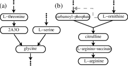
Figure 3: Converging pathways. (a) Glycine is synthesized in two independent pathways. (b) Citrulline is synthesized from products of two pathways. Abbreviations: 2A3O, 2-Amino-3-oxobutanoate.

3.5 Converging pathways – reaction with two fluctuating substrates

As mentioned above, some reactions in a biosynthesis pathway involve side-reactants, which are assumed to be abundant (and hence at a constant level). Let us now discuss briefly a case where this approach fails. Suppose that the two products of two linear pathways serve as precursors for one reaction. This, for example, is the case in the arginine biosynthesis pathway, where L-ornithine is combined with carbamoyl-phosphate by ornithine-carbamoyltransferase to create citrulline (figure 3(b)) [24]. Within a flux balance model, the net fluxes of both substrates must be equal to achieve steady state, in which case the macroscopic Michaelis-Menten flux takes the form

$$c=v_{\max}\frac{[S_{1}][S_{2}]}{(K_{M1}+[S_{1}])(K_{M2}+[S_{2}])}\;.$$

Here $[S_{1,2}]$ are the steady-state concentrations of the two substrates, and $K_{M1,2}$ the corresponding MM-constants. However, flux balance provides only one constraint to a system with two degrees of freedom.

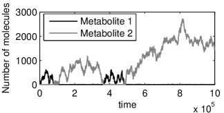
Figure 4: Time course of a two-substrate enzymatic reaction, as obtained by a Gillespie simulation [44]. Here $c=3t^{-1}$, $k_{+}=5t^{-1}$ and $k_{-}=2t^{-1}$ for both substrates, $t$ being an arbitrary time unit.

In fact, this reaction exhibits no steady state. To see why, consider a typical time evolution of the two substrate pools (figure 4). Suppose that at a certain time one of the two substrates, say $S_{1}$, is of high molecule-number compared with its equilibrium constant, $m_{1}\gg K_{1}$. In this case, the product synthesis rate is unaffected by the precise value of $m_{1}$, and is given approximately by $v_{\max}m_{2}/(m_{2}+K_{2})$. Thus, the number $m_{2}$ of $S_{2}$ molecules can be described by the single-substrate reaction analyzed above, while $m_{1}$ performs a random walk (under the influence of a weak logarithmic potential), which is bound to return, after some time $\tau$, to values comparable with $K_{1}$. Then, after a short transient, one of the two substrates will become unlimiting again, and the system will be back in the scenario described above, perhaps with the two substrates changing roles (depending on the ratio between $K_{1}$ and $K_{2}$).

Importantly, the probability for the time $\tau$ during which one of the substrates is at saturating concentration scales as $\tau^{-3/2}$ for large $\tau$. During this time the substrate pool may increase to the order $\sqrt{\tau}$. The fact that $\tau$ has no finite mean implies that this reaction has no steady state. Since accumulation of any substrate is most likely toxic, the cell must provide some other mechanism to limit these fluctuations. This may be one interpretation for the fact that within the arginine biosynthesis pathway, L-ornithine is an enhancer of carbamoyl-phosphate synthesis (dashed line in figure 3(b)).

In contrast, a steady-state always exists if the two metabolites experience linear degradation, as this process prevents indefinite accumulation. However, in general one expects enzymatic reactions to dominate over futile degradation. In this case, equal in-fluxes of the two substrates result in large fluctuations, similar to the ones described above [31].

4 Discussion

In this work we have characterized stochastic fluctuations of metabolites for dominant simple motifs of the metabolic network in the steady state. Motivated by the analogy between the directed biochemical pathway and the mass transfer model or, equivalently, as the queueing network, we show that the intermediate metabolites in a linear pawthway – the key motif of the biochemical netrowk – are statistically independent. We then extend this result to a wide range of pathway structures. Some of the results (e.g., the directed linear, diverging and cyclic pathways) have been proven previously in other contexts. In other cases (e.g., for reversible reaction, diverging pathway or with leakage/dilution), the product measure is not exact. Nevertheless, based on insights from the exactly solvable models, we conjecture that it still describes faithfuly the statistics of the pathway. Using the product measure as an Ansatz, we obtained quantitative predictions which turned out to be in excellent agreement with the numerics (figure 2). These results suggest that the product measure may be an effective starting point for quantitative, non-perturbative analysis of (the stochastic properties) of these circuit/networks. We hope this study will stimulate further analytical studies of the large variety of pathway topologies in metabolic networks, as well as in-depth mathematical analysis of the conjectured results. Moreover, it will be interesting to explore the applicability of the present approach to other cellular networks, in particular, stochasticity in protein signaling networks [2], whose basic mathematical structure is also a set of interlinked Michaelis-Menton reactions.

Our main conclusion, that the steady-state fluctuations in each metabolite depends only on the properties of the reactions consuming that metabolite and not on fluctuations in other upstream metabolites, is qualitatively different from conclusions obtained for gene networks in recent studies, e.g., the “noise addition rule” [14, 15] derived from the Independent Noise Approximation, and its extension to cases where the singnals and the processing units interact [17]. The detailed analysis of [17], based on the Linear Noise Approximation found certain anti-correlation effects which reduced the extent of noise propagation from those expected by “noise addition” alone [14, 15]. While the specific biological systems studied in [17] were taken from protein signaling systems, rather than metabolic networks, a number of systems studied there are identical in mathematical structure to those considered in this work. It is reassuring to find that reduction of noise propagation becomes complete (i.e., no noise propagation) according to the analysis of [17], also, for Poissonian input noise where direct comparisons can be made to our work (ten Wolde, private communication). The cases in which residue noise propagation remained in [17], corresponded to certain “bursty” noises which is non-Poissonian. While bursty noise is not expected for metabolic and signaling reactions, it is nevertheless important to address the extent to which the main finding of this work is robust to the nature of stochasticity in the input and the individual reactions. The exact result on the cyclic pathways and the numerical result on the directed pathway with feedback inhibition suggest that our main conclusion on statistical independence of the different nodes extends significantly beyond strict Poisson processes. Indeed, generalization that preserve this property include classes of transport rules and extended topologies [37, 38].

The absence of noise propagation for a large part of the metabolic network allows intermediate metabolites to be shared freely by multiple reactions in multiple pathways, without the need of installing elaborate control mechanisms. In these systems, dynamic fluctuations (e.g., stochasticity in enzyme expression which occurs at a much longer time scale) stay local to the node, and are shielded from triggering system-level failures (e.g., grid-locks). Conversely, this property allows convenient implementation of controls on specific node of pathways, e.g., to limit the pool of a specific toxic intermediate, without the concern of elevating fluctuations in other nodes. We expect this to make the evolution of metabolic network less constrained, so that the system can modify its local properties nearly freely in order to adapt to environmental or cellular changes. The optimized pathways can then be meshed smoothly into the overall metabolic network, except for junctions between pathways where complex fluctuations not constrained by flux conservation.

In recent years, metabolomics, i.e., global metabolite profiling, has been suggested as a tool to decipher the structure of the metabolic network [39, 40]. Our results suggest that in many cases, steady-state fluctuations do not bare information about the pathway structure. Rather, correlations between metabolite fluctuations may be, for example, the result of fluctuation of a common enzyme or coenzyme, or reflect dynamical disorder [27]. Indeed, a bioinformatic study found no straightforward connection between observed correlation and the underlying reaction network [41]. Instead, the response to external perturbation [28, 39, 42] may be much more effective in shedding light on the underlying structure of the network, and may be used to study the morphing of the network under different conditions. It is important to note that all results described here are applicable only to systems in the steady state; transient responses such as the establishment of the steady state and the response to external perturbations will likely exhibit complex temporal as well as spatial correlations. Nevertheless, it is possible that some aspects of the response function may be attainable from the steady-state fluctuations through non-trivial fluctuation-dissipation relations as was shown for other related nonequilibrium systems [22, 43].

Supporting Material

Appendix A Microscopic model

Under the assumption of fast equlibration between the substrate and the enzyme, the probability of having $N_{SE}$ complexes given $m$ substrate molecules and $N_{E}$ enzymes is given by equation ( 3 ) of the main text. To write the partition function explicitly, we define $u(x)=U(x,1-m-N_{E};-K)$, where $U$ denotes the Confluent Hypergeometric function [45]. One can then write the partition sum as $Z_{m,N_{E}}=(-K)^{-N_{E}}u(-m)$. The turnover rate is then given by $w_{m}=\frac{k_{2}N_{E}}{V}[-m\,u(1-m)]/[u(-m)]$, which can be approximated by Equation ( 4 ).

Appendix B Influx of metabolites

A metabolic reaction in vivo can be described as turnover of an incoming flux of substrate molecules, characterized by a Possion process with rate $c$, into an outgoing flux. To find the probability of having $m$ substrate molecules we write down the Master equation,

$$\frac{d}{dt}\pi(m)=\left[c(a-1)+(\hat{a}-1)w_{m}\right]\pi(m)=c[\pi(m-1)-\pi(m)]+[w_{m+1}\pi(m+1)-w_{m}\pi(m)]\;,$$ (14)

where we took the opportunity to define the lowering and raising operators $a$ and $\hat{a}$, which – for any function $h(n)$ – satisfy $ah(n)=h(n-1)$, $ah(0)=0$, and $\hat{a}h(n)=h(n+1)$. The first term in this equation is the influx, and the second is the biochemical reaction. The solution of this steady state equation is of the form $\pi(m)\sim c^{m}/\prod_{k=1}^{m}{w_{k}}$ (up to a normalization constant), as can be verified by plugging it into the equation,

$$\left[c\left(\frac{\pi(m-1)}{\pi(m)}-1\right)+\left(\frac{\pi(m+1)}{\pi(m)}w_{m+1}-w_{m}\right)\right]=c\left(\frac{w_{m}}{c}-1\right)+\left(\frac{c}{w_{m+1}}w_{m+1}-w_{m}\right)=0.$$ (15)

Using the approximate form of $w_{m}$, as given in ( 4 ), the probability $\pi(m)$ takes the form,

$$\pi(m)={m+K+(N_{E}-1)\choose m}(1-z)^{K+N_{E}}z^{m}\;,$$ (16)

as given in equation ( 5 ) of the main text.

Appendix C Directed linear pathway

We now derive our key results, equation ( 8 ) (The result has been derived previously in the context of queueing networks [46], and of mass-transport systems [47]). To this end we write the Master equation for the joint probability function $\pi\equiv\pi(m_{1},m_{2},\cdots,m_{L})$,

$$\frac{d}{dt}{\pi}=\left[c(a_{1}-1)+\sum_{i=1}^{L-1}(\hat{a}_{i}a_{i+1}-1)w^{(i)}_{m_{i}}+(\hat{a}_{L}-1)w^{(L)}_{m_{L}}\right]\pi\;,$$ (17)

which generalizes ( 14 ). As above, $a_{i}$ and $\hat{a_{i}}$ are lowering and raising operators, acting on the number of $S_{i}$ molecules. The first term in this equation is the incoming flux $c$ of the substrate, and the last term is the flux of end product. Let us try to solve the steady-state equation by plugging a solution of the form $\pi(m_{1},m_{2},\cdots,m_{L})=\prod g_{i}(m_{i})$, yielding

$$\\ c[\frac{g_{i}(m_{1}-1)}{g_{1}(m_{1})}-1]+\sum_{i=1}^{L-1}[w^{(i)}_{m_{i}+1}\frac{g_{i}(m_{i}+1)g_{i+1}(m_{i+1}-1)}{g_{i}(m_{i})g_{i+1}(m_{i+1})}-w^{(i)}_{m_{i}}]+[w^{(L)}_{m_{L}+1}\frac{g_{L}(m_{L}+1)}{g_{L}(m_{L})}-w^{(L)}_{m_{L}}]=0\;.$$ (18)

Motivated by the solution to ( 14 ), we try to satisfy this equation by choosing $g_{i}(m)=c^{m}/\prod_{k=1}^{m}w^{(i)}_{k}$. With this choice we have $g(m+1)/g(m)=c/w_{m+1}$ and $g(m-1)/g(m)=w_{m}/c$. It is now straightforward to verify that indeed

$$c\left(\frac{w^{(1)}_{m_{1}}}{c}-1\right)+\sum_{i=1}^{L-1}\left(w^{(i+1)}_{m_{i+1}}-w^{(i)}_{m_{i}}\right)+\left(c-w^{(L)}_{m_{L}}\right)=0\;.$$ (19)

Finally, in our choice of $g_{i}(m)$ we replace $w^{(i)}_{m}$ by the MM- rate $v_{i}m_{i}/(m_{i}+K_{i})$, and find that in fact $g_{i}(m)=\pi_{i}(m)$, namely

$$\pi(m_{1},m_{2},\ldots,m_{L})=\prod_{i=1}^{L}\pi_{i}(m_{i})\;,$$ (20)

as stated in ( 8 ).

Appendix D End-product inhibition

Equation ( 13 ) of the main text is a self-consistent equation for the steady- state flux $c$ through a pathway regulated via end-product inhibition. Using considerations analogous to what led to the exact result on the product measure distribution for the cyclic pathways, we conjecture that even for the present case of end-product inhibition, the distribution function can still be approximated by the product measure ( 20 ) with the form of the single node distributions given by ( 16 ). The flux $c$ enters the calculation of the average on the right-hand side through the probability function $\pi(m)$. Solving this equation for $c$ yields the steady state current, and consequently determines the mean occupancy and standard deviation of all intermediates.

To verify the validity of this conjecture, and to demonstrate its application, we consider the case $h=1$. In this case one can carry the sum, and find

$$c = \sum_{m_{L}=0}^{\infty}c_{0}\left[1+(m_{L}/K_{I})^{h}\right]^{-1}\pi_{L}(m_{L})$$

$$= c_{0}(1-z)^{K_{L}}{{}_{2}F_{1}}(K_{I},K_{L};K_{I}+1;z)$$

with $z=c/v_{L}$ and ${}_{2}F_{1}$ the hypergeometric function [45]. This equation was solved numerically, and plotted in supporting figure 6(a) for some values of $K_{I}$ and $K_{L}$. Note that predictions based on the product measure (lines) are in excellent agreement with the results of numerical simulation (circles) for the different sets of parameters tried.

Results obtained from equation ( D ) can be used, for example, to compare the flux that flows through the noisy pathway with the mean-field flux $c_{\rm MF}$, obtained when one ignores fluctuations in $m_{L}$, i.e.,

$$c_{\rm MF}=\frac{c_{0}}{1+(s_{L}/K_{I})^{h}}\;.$$ (22)

The fractional difference $\delta c=(c-c_{\rm MF})/c_{\rm MF}$ is plotted in supporting figure 6(b). The results show that number fluctuations in the end-product always increase the flux in the pathway since $\delta c>0$ always. Quantitatively, this increase can easily be several percent. For large $c_{0}$, a simplifying expression can be derived by using an asymptotic expansion of the hypergeometric function [45]. For example, when $K_{I}<K_{L}$,

$$(1-z)^{K_{L}}{{}_{2}F_{1}}(K_{I},K_{L};K_{I}+1;z)\sim\frac{v_{L}K_{L}}{1+K_{L}-K_{I}}\;,$$ (23)

which yields

$$\frac{c-c_{\rm MF}}{c_{\rm MF}}\sim\frac{1}{K_{I}}\frac{v_{L}}{c_{0}}\;.$$ (24)

Thus the effect of end-product fluctuations on the current is enhanced by stronger binding of the inhibitor (smaller $K_{I}$), as one would expect. We note that obtaining these predictions from Monte-Carlo simulation is rather difficult, given the fact that one is interested here in sub-leading quantities.

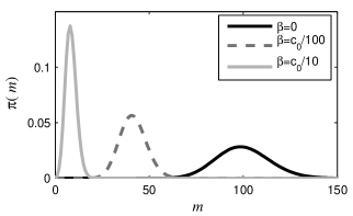
Figure 5: The steady-state distribution $\pi(m)$ of a metabolite, that experiences enzymatic reaction (with rate $w_{m}=vm/(m+K-1)$) and linear degradation (with rate $\beta m$), as given by equation ( 10 ) of the main text. Here $K=100$ and $v=2c_{0}$.

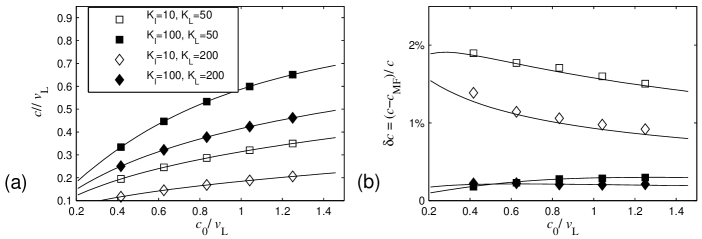
Figure 6: Pathway with end-product inhibition. The influx rate is taken to be $c_{0}/(1+m_{L}/K_{I})$, and thus the steady-state flux is given by equation ( 12 ) of the main text, with $h=1$. (a) Assuming that different metabolites in the pathway remain decoupled even in the presence of feedback regulation, ( 12 ) can be approximated by ( D ). Numerical solutions of equation ( D ) (lines) are compared with Monte-Carlo simulations (symbols). Values of parameters are chosen randomly such that $100<K_{i}<1000$ and $c<v_{i}<10c$. For the data presented here, $v_{L}=2.4c$. We find that ( D ) yields excellent prediction for the steady-state flux. (b) Neglecting fluctuations altogether yields a mean-field approximation for the flux, $c_{\rm MF}$, given in ( 22 ). For the same data of (a), we plot the fractional difference $\delta_{c}=(c-c_{\rm MF})/c$. We find that steady-state flux is increased by fluctuations, and thus taking fluctuations into account (even in an approximate manner) better predicts the steady-state flux.

References

References

- [1] Zhou, T., Chen, L. & Aihara, K. (2005) Phys. Rev. Lett. 95, 178103.
- [2] Colman-Lerner A, Gordon A, Serra E, Chin T, Resnekov O, Endy D, Pesce CG, Brent R. (2005) Nature 437: 699-706.
- [3] Raser, J.M. & O’shea, E.K. (2005) Science 309, 2010.
- [4] Kaern, M., Elston, T.C., Blake, W.J. & Collins, J.J. (2005) Nat. rev. Gen. 6, 451.
- [5] Kussel, E. & Leibler, S. (2005) Science 309, 2075.
- [6] Suel, G.M., Garcia-Ojalvo, J., Liberman, L.M., & Elowitz M.B. (2006) Nature 440, 545.
- [7] Fell, D. (1997) Understanding the Control of Metabolism (Protland Press, London, England).
- [8] Swain, P.S., Elowitz, M.B. & Siggia E.D. (2002) Proc Natl Acad Sci U S A 99, 12795.
- [9] Pedraza, J.M. & van Oudenaarden, A. (2005) Science 307, 1965.
- [10] Golding, I., Paulsson, J., Zawilski, S.M., & Cox E.C. (2005) Cell 123, 1025.
- [11] Thattai, M. & van Oudenaarden, A. (2002) Biophys J 82, 2943-50.
- [12] Hooshangi, S., Thiberge, S. & Weiss, R. (2005) Proc Natl Acad Sci U S A 102, 3581-6.
- [13] Hooshangi, S. & Weiss, R. (2006) Chaos 16, 026108.
- [14] Paulsson, J. (2004) Nature 427, 415.
- [15] Shibata, T. & Fujimoto, K., Proc Natl Acad Sci U S A 102, 331.
- [16] Austin D.W., Allen M.S., McCollum J.M., Dar R.D., Wilgus J.R., Sayler G.S., Samatova N.F., Cox C.D., & Simpson M.L (2006) Nature 439, 608-11
- [17] Tanase-Nicola, S., Warren, P.B., & ten Wolde P.R. (2006) Phys Rev Lett 97 068102.
- [18] Sasai M. & Wolynes P.G. (2003) Proc Natl Acad Sci U S A 100, 2374-9.
- [19] Michal, G. (1999) Biochemical Pathways (Wiley & Sons, New York).
- [20] Berg J.M, Tymoczko J.L., & Stryer L. (2006) Bichemistry, 6th edition, (WH Freeman Ĉompany, New York)
- [21] Taylor, H.M. & Karlin, S. (1998) An Introduction to Stochastic Modeling, 3rd edition (Academic Press); Ross, S.M. (1983) Stochastic Processes (John Wiley & Sons).
- [22] Liggett, T.M. (1985) Interacting Particle Systems (Springer-Verlag, New York).
- [23] Levine, E. , Mukamel, D. & Schütz, G.M. (2005) J. Stat. Phys. 120, 759.
- [24] Neidhardt, F.C. et al, eds. (1996) Escherichia coli and Salmonella: Cellular and Molecular Biology, 2nd ed. (Am. Soc. Microbiol., Washington, DC).
- [25] McAdams, H.H. & Arkin, A. (1997) Proc. Natl. Acad. Sci. USA 94, 814.
- [26] Xie, X.S. & Lu, H.P. (1999) J Biol. Chem. 274, 15967.
- [27] English, B.P., Min, W., van Oijen, A.M., Lee, K.T., Luo, G., Sun, H., Cherayil, B.J., Kou, S.C. & Xie., X.S. (2005) Nat. Chem. Bio. 2, 87.
- [28] Arkin, A. Shen, P. & Ross, J. (1997) from measurements, Science 29, 1275.
- [29] Kou, S.C., Cherayil, B.J., Min, W., English, B.P. & Xie, X.S. (2005) J. Phys. Chem. B 109, 19068.
- [30] Qiana, H. & Elson, E.L. (2002) Biophys. Chem. 101-102, 565.
- [31] Elf, J., Paulsson, J., Berg, O.G. & Ehrenberg, M. (2003) Biophys. J 84, 154.
- [32] Edwards, J.S., Covert, M. & Palsson B.O. (2002) Environ Microbiol. 4, 133.
- [33] Evans, M. R. & Hanney, T. (2005) J. Phys. A 38, R195.
- [34] Jackson, J.R. (1957) Operations Research 5, 58.
- [35] Spitzer, F. (1970) Adv. Math. 5, 246.
- [36] LaPorte D.C., Walsh K., & Koshland, Jr D.E (1984) J. Biochem. 259 14068.
- [37] Evans M.R., Majumdar S.N., & Zia R.K.P (2004) J. Phys. A: Math. Gen. 37 L275.
- [38] Greenblatt, R.L., & Lebowitz, J.L. (2006), J. Phys. A: Math. Gen. 39 1565 1573.
- [39] Arkin, A. & Ross, J. (1995) Measured Time-Series, J. Phys. Chem. 99, 970.
- [40] Weckwerth, W. & Fiehn, O. (2002) Curr. Opin. Biotech. 13, 156.
- [41] Steuer, R., Kurths, J., Fiehn, O. & Weckwerth, W.(2003) Bioinformatics 19, 1019.
- [42] Vance, W., Arkin, A. & Ross, J. (2002) networks, Proc. Natl. Acad. Sci. USA 99, 5816.
- [43] Forster, D. , Nelson, D., & Stephens, M. (1977) Phys. Rev. A 16, 732 749
- [44] Gillespie, D.T. (1977). J. Phys. Chem 81, 2340.
- [45] M. Abramowitz, Handbook of Mathematical Functions (Dover, New York, 1972).
- [46] Taylor, H.M. & Karlin, S. (1998) An Introduction to Stochastic Modeling, 3rd edition (Academic Press); Ross, S.M. (1983) Stochastic Processes (John Wiley & Sons).
- [47] Levine, E. , Mukamel, D. & Schütz, G.M. (2005) J. Stat. Phys. 120, 759.