A new search for planet transits in NGC~6791.

Abstract

Context. Searching for planets in open clusters allows us to study the effects of dynamical environment on planet formation and evolution.

Aims. Considering the strong dependence of planet frequency on stellar metallicity, we studied the metal rich old open cluster NGC~6791 and searched for close-in planets using the transit technique.

Methods. A ten-night observational campaign was performed using the Canada-France-Hawaii Telescope (3.6m), the San Pedro Mártir telescope (2.1m), and the Loiano telescope (1.5m). To increase the transit detection probability we also made use of the Bruntt et al. (2003) eight-nights observational campaign. Adequate photometric precision for the detection of planetary transits was achieved.

Results. Should the frequency and properties of close-in planets in NGC~6791 be similar to those orbiting field stars of similar metallicity, then detailed simulations foresee the presence of 2-3 transiting planets. Instead, we do not confirm the transit candidates proposed by Bruntt et al. (2003). The probability that the null detection is simply due to chance coincidence is estimated to be $3$%-$10$%, depending on the metallicity assumed for the cluster.

Conclusions. Possible explanations of the null-detection of transits include: (i) a lower frequency of close-in planets in star clusters; (ii) a smaller planetary radius for planets orbiting super metal rich stars; or (iii) limitations in the basic assumptions. More extensive photometry with $3$–$4$m class telescopes is required to allow conclusive inferences about the frequency of planets in NGC~6791.

1 Introduction

During the last decade more than 200 extra-solar planets have been discovered. However, our knowledge of the formation and evolution of planetary systems remains largely incomplete. One crucial consideration is the role played by environment where planetary systems may form and evolve.

More than 10% of the extra-solar planets so far discovered are orbiting stars that are members of multiple systems (Desidera & Barbieri 2007). Most of these are binaries with fairly large separations (a few hundred AU). However, in few cases, the binary separation reaches about 10 AU (Hatzes et al. hatzes03 (2003); Konacki 2005), indicating that planets can exist even in the presence of fairly strong dynamical interactions.

Another very interesting dynamical environment is represented by star clusters, where the presence of nearby stars or proto-stars may affect the processes of planet formation and evolution in several ways. Indeed, close stellar encounters may disperse the proto-planetary disks during the fairly short (about 10 Myr, e.g., Armitage et al. armitage03 (2003)) epoch of giant planet formation or disrupt the planetary system after its formation (Bonnell et al. bonnell01 (2001); Davies & Sigurdsson davies01 (2001); Woolfson woolfson04 (2004); Fregeau et al. fregeau06 (2006)). Another possible disruptive effect is the strong UV flux from massive stars, which causes photo-evaporation of dust grains and thus prevents planet formation (Armitage armitage00 (2000); Adams et al. adams04 (2004)). These effects are expected to depend on star density, being much stronger for globular clusters (typical current stellar density $\sim 10^{3}$ stars pc^-3) than for the much sparser open clusters ($\leq 10^{2}$ stars pc^-3).

The recent discovery of a planet in the tight triple system HD$188753$ (Konacki konacki (2005)) adds further interest to the search for planets in star clusters. In fact, the small separation between the planet host HD$188753$A and the pair HD$188753$BC (about 6 AU at periastron) makes it very challenging to understand how the planet may have been formed (Hatzes & Wüchterl hatzes05 (2005)). Portegies, Zwart & McMillan et al. (zwart05 (2005)) propose that the planet formed in a wide triple within an open cluster and that dynamical evolution successively modified the configuration of the system. Without observational confirmation of the presence of planets in star clusters, such a scenario is purely speculative.

On the observational side, the search for planets in star clusters is a quite challenging task. Only the closest open clusters are within reach of high-precision radial velocity surveys (the most successful planet search technique). However, the activity-induced radial velocity jitter limits significantly the detectability of planets in clusters as young as the Hyades (Paulson et al. paulson (2004)). Hyades red giants have a smaller activity level, and the first planet in an open cluster has been recently announced by Sato et al. (2007), around $\epsilon\,$ Tau.

The search for photometric transits appears a more suitable technique: indeed it is possible to monitor simultaneously a large number of cluster stars. Moreover, the target stars may be much fainter. However, the transit technique is mostly sensitive to close-in planets (orbital periods $\leq$ 5 days).

Space and ground-based wide-field facilities were also used to search for planets in the globular clusters 47 Tucanae and $ω$ Centauri. These studies (Gilliland et al.~gilliland (2000); Weldrake et al.~weldrake05 (2005); Weldrake et al. 2006) reported not a single planet detection. This seemed to indicate that planetary systems are at least one order of magnitude less common in globular clusters than in Solar vicinity. The lack of planets in 47 Tuc and $ω$ Cen may be due either to the low metallicity of the clusters (since planet frequency around solar type stars appears to be a rather strong function of the metallicity of the parent star: Fischer & Valenti fischer05 (2005); Santos et al. santos04 (2004)), or to environmental effects caused by the high stellar density (or both).

One planet has been identified in the globular cluster M4 (Sigurdsson et al. sigurdsson03 (2003)), but this is a rather peculiar case, as the planet is in a circumbinary orbit around a system including a pulsar and it may have formed in a different way from the planets orbiting solar type stars (Beer et al. beer04 (2004)).

Open clusters are not as dense as globular clusters. The dynamical and photo-evaporation effects should therefore be less extreme than in globular clusters. Furthermore, their metallicity (typically solar) should, in principle, be accompanied by a higher planet frequency.

In the past few years, some transit searches were specifically dedicated to open clusters: see e.g. von Braun et al. (vonbraun05 (2005)), Bramich et al. (bramich05 (2005)), Street et al. (street (2003)), Burke et al. (2006), Aigrain et al. (2006) and references therein. However, in a typical open cluster of Solar metallicity with $\sim 1000$ cluster members, less than one star is expected to show a planetary transit. This depends on the assumption that the planet frequency in open clusters is similar to that seen for nearby field stars . Considering the unavoidable transits detection loss due to the observing window and photometric errors, it turns out that the probability of success of such efforts is fairly low unless several clusters are monitored .

On the other hand, the planet frequency might be higher for open clusters with super-solar metallicities. Indeed, for [Fe/H] between $+0.2$ and $+0.4$ the planet frequency around field stars is 2-6 times larger than at solar metallicity. However, only a few clusters have been reported to have metallicities above [Fe/H]$=+0.2$. The most famous is NGC~$6791$, a quite massive cluster that is at least $8$ Gyr old (Stetson et al. stetson03 (2003); King et al. king05 (2005), and Carraro et al. carraro06 (2006)). As estimated by different authors, its metallicity is likely above [Fe/H]=$+0.2$ (Taylor taylor01 (2001)) and possibly as high as [Fe/H]=$+0.4$ (Peterson et al. peterson (1998)). The most recent high dispersion spectroscopy studies confirmed the very high metallicity of the cluster ([Fe/H]=$+0.39$, Carraro et al. carraro06 (2006); [Fe/H]=$+0.47$, Gratton et al. gratton06 (2006)). Its old age implies the absence of significant photometric variability induced by stellar activity. Furthermore, NGC~6791 is a fairly rich cluster. All these facts make it an almost ideal target.

NGC~6791 has been the target of two photometric campaigns aimed at detecting planets transits. Mochejska et al. (mochejska02 (2002), mochejska05 (2005), hereafter M05) observed the cluster in the R band with the 1.2 m Fred Lawrence Whipple Telescope during 84 nights, over three observing seasons (2001-2003). They found no planet candidates, while the expected number of detections considering their photometric precision and observing window was $\sim 1.3$. Bruntt et al. (bruntt03 (2003), hereafter B03) observed the cluster for 8 nights using ALFOSC at NOT. They found 10 transit candidates, most of which (7) being likely due to instrumental effects.

Nearly continuous, multi-site monitoring lasting several days could strongly enhance the transit detectability. This idea inspired our campaigns for multi-site transit planet searches in the super metal rich open clusters NGC~6791 and NGC~6253. This paper presents the results of the observations of the central field of NGC~6791, observed at CFHT, San Pedro Mártir (SPM), and Loiano. We also made use of the B03 data-set [obtained at the Nordic Optical Telescope (NOT) in $2001$] and reduce it as done for our three data-sets. The analysis for the external fields, containing mostly field stars, and of the NGC~6253 campaign, will be presented elsewhere.

The outline of the paper is the following: Sect. 2 presents the instrumental setup and the observations. We then describe the reduction procedure in Sect. 3, and the resulting photometric precision for the four different sites is in Sect. 4. The selection of cluster members is discussed in Sect. 5. Then, in Sect. 6, we describe the adopted transit detection algorithm. In Sect. 7 we present the simulations performed to establish the transit detection efficiency (TDE) and the false alarm rate (FAR) of the algorithm for our data-sets. Sect. 8 illustrates the different approaches that we followed in the analysis of the data. Sect. 9 gives details about the transit candidates.

In Sect. 10, we estimate the expected planet frequency around main sequence stars of the cluster, and the expected number of detectable transiting planets in our data-sets. In Sect. 11, we compare the results of the observations with those of the simulations, and discussed their significance. In Sect. 12 we discuss the different implications of our results, and, in Sect. 13, we make a comparison with other transit searches toward NGC~6791. In Sect. 14 we critically analyze all the observations dedicated to the search for planets in NGC~6791 so far, and propose future observations of the cluster, and finally, in Sect. 15, we summarize our work.

2 Instrumental setup and observations

The observations were acquired during a ten-consecutive-day observing campaign, from July 4 to July 13, 2002. Ideally, one should monitor the cluster nearly continuously. For this reason, we used three telescopes, one in Hawaii, one in Mexico, and the third one in Italy. In Table 1 we show a brief summary of our observations.

In Hawaii, we used the CFHT with the CFH12K detector , a mosaic of 12 CCDs of 2048$\times$4096 pixels, for a total field of view of 42$\times$28 arcmin, and a pixel scale of $0.206$ arcsec/pixel. We acquired $278$ images of the cluster in the $V$ filter. The seeing conditions ranged between $0\aas@@fstack{\prime\prime}6$ to $1\aas@@fstack{\prime\prime}9$, with a median of $1\aas@@fstack{\prime\prime}0$. Exposure times were between $200$ and $900$ sec, with a median value of $600$ sec. The observers were H. Bruntt and P.B. Stetson.

In San Pedro Mártir, we used the 2.1m telescope, equipped with the Thomson 2k detector. However the data section of the CCD corresponded to a $1k\,\times\,1k$ pixel array. The pixel scale was 0.35 arcsec/pixel, and therefore the field of view ($\sim$ 6 arcmin²) contained just the center of the cluster, and was smaller than the field covered with the other detectors. We made use of $189$ images taken between July 6, 2002 and July 13, 2002. During the first two nights the images were acquired using the focal reducer, which increased crowding and reduced our photometric accuracy. All the images were taken in the $V$ filter with exposure times of $480-1200$ sec (median $660$ sec), and seeing between $1\aas@@fstack{\prime\prime}1$ and $2\aas@@fstack{\prime\prime}1$ (median $1\aas@@fstack{\prime\prime}4$). Observations were taken by A. Arellano Ferro.

In Italy, we used the Loiano 1.5m telescope equipped with BFOSC + the EEV 1300$\times$1348B detector. The pixel scale was 0.52 arcsec/pixel, for a total field coverage of 11.5 arcmin². We observed the target during four nights ($2002$ July $6-9$). We acquired and reduced $63$ images of the cluster in the $V$ and Gunn $i$ filters ($61$ in $V$, $2$ in $i$). The seeing values were between $1\aas@@fstack{\prime\prime}1$ and $4\aas@@fstack{\prime\prime}3$ arcsec, with a median value of $1\aas@@fstack{\prime\prime}4$ arcsec. Exposure times ranged between 120 and 1500 sec (median $1080$ sec). The observer was S. Desidera.

We also make use of the images taken by B03 in 2001. We obtained these images from the Nordic Optical Telescope (NOT) archive. As explained in BO3, these data covered eight nights between July 9 and 17, 2001. The detector was ALFOSC a 2k$\times$2k thinned Loral CCD with a pixel scale of 0.188 arcsec/pixel yielding a total field of view of 6.5 arcmin². Images were taken in the $I$ and $V$ filters with a median seeing of $1$ arcsec. We used only the images of the central part of the cluster (which were the majority) excluding those in the external regions. In total we reduced $227$ images in the $V$ filter and $389$ in the $I$ filter.

It should be noted that ALFOSC and BFOSC are focal reducers, hence light concentration introduced a variable background. These effects can be important when summed with flat fielding errors. In order to reduce these un-desired effects, the images were acquired while trying to maintain the stars in the same positions on the CCDs. Nevertheless, the precision of this pointing procedure was different for the four telescopes: the median values of the telescope shifts are of $0\aas@@fstack{\prime\prime}5$, $0\aas@@fstack{\prime\prime}5$, $3\aas@@fstack{\prime\prime}4$ and $2\aas@@fstack{\prime\prime}1$, respectively for Hawaii, NOT, SPM, and Loiano. This means that while for the CFHT and the NOT the median shift was at a sub-seeing level (half of the median seeing), for the other two telescopes it was respectively of the order of 2.4 and 1.5 times the median seeing. Hence, it is possible that flat-fielding errors and possible background variation have affected the NOT, SPM, and Loiano photometry, but the effects on the Hawaii photometry are expected to be smaller.

Table 1: Summary of the observations taken during $4$-$13$ July, $2002$ in Hawaii, San Pedro Màrtir, Loiano and from $9$-$17$ July, $2001$ in La Palma (by B03).

	Hawaii	San Pedro Mártir	Loiano	NOT
N. of Images	278	189	63	227(V), 389(I)
Nights	8	8	4	8
Scale (arcsec/pix)	0.21	0.35	0.52	0.188
FOV (arcmin)	42 x 28	6 x 6	11.5 x 11.5	6.5 x 6.5

Bad weather conditions and the limited time allocated at Loiano Observatory caused incomplete coverage of the scheduled time interval. Moreover we did not use the images coming from the last night (eighth night) of observation in La Palma with the NOT because of bad weather conditions. Our observing window, defined as the interval of time during which observations were carried out, is shown in Tab. 3 for Hawaii, SPM and Loiano observations and in Tab. 3 for La Palma observations.

Table 2: The observing window relative to the July $2002$ observations. The number of observing hours is given for each night. The last line shows the total number of observing hours for each site.

Night	Hawaii	SPM	Loiano
$1^{st}$	$3.58$	$-$	$-$
$2^{nd}$	$3.88$	$-$	$-$
$3^{rd}$	$2.68$	$6.31$	$3.58$
$4^{th}$	$7.56$	$6.61$	$5.21$
$5^{th}$	$5.23$	$6.58$	$6.08$
$6^{th}$	$8.30$	$6.86$	$5.45$
$7^{th}$	$-$	$3.20$	$-$
$8^{th}$	$-$	$7.03$	$-$
$9^{th}$	$8.34$	$7.27$	$-$
$10^{th}$	$8.37$	$4.15$	$-$
Total	$47.94$	$48.01$	$20.32$

Table 3: The observing window relative to the July $2001$ observations.

Night	La Palma
$1^{st}$	$5.45$
$2^{nd}$	$7.06$
$3^{rd}$	$8.04$
$4^{th}$	$7.61$
$5^{th}$	$7.57$
$6^{th}$	$7.82$
$7^{th}$	$7.72$
$8^{th}$	$2.41$
Total	$53.68$

3 The reduction process

3.1 The pre-reduction procedure

For the San Pedro, Loiano and La Palma images, the pre-reduction was done in a standard way, using IRAF routines. The images from the Hawaii came already reduced via the ELIXIR software.

3.2 Reduction strategies

The data-sets described in Sec. 2 were reduced with three different techniques: aperture photometry, PSF fitting photometry and image subtraction. An accurate description of these techniques is given in the next Sections. Our goal was to compare their performances to see if one of them performed better than the others. For what concerned aperture and PSF fitting photometry we used the DAOPHOT (Stetson 1987) package. In particular the aperture photometry routine was slightly different from that one commonly used in DAOPHOT and was provided by P .B. Stetson. It performed the photometry after subtracting all the neighbors stars of each target star. Image subtraction was performed by means of the ISIS2.2 package (Alard & Lupton, 1998) except for what concerned the final photometry on the subtracted images which was performed with the DAOPHOT aperture routine for the reasons described in paragraph 3.4.

3.3 DAOPHOT/ALLFRAME reduction: aperture and PSF fitting photometry

The DAOPHOT/ALLFRAME reduction package has been extensively used by the astronomical community and is a very well tested reduction technique. The idea behind this stellar photometry package consists in modelling the PSF of each image following a semi-analytical approach, and in fitting the derived model to all the stars in the image by means of least square method. After some tests, we chose to calculate a variable PSF across the field (quadratic variability). We selected the first $200$ brightest, unsaturated stars in each frame, and calculated a first approximate PSF from them. We then rejected the stars to which DAOPHOT assigned anomalously high fitting $\chi$ values. After having cleaned the PSF star list, we re-calculated the PSF. This procedure was iterated three times in order to obtain the final PSF for each image.

We then used DAOMATCH and DAOMASTER (Stetson 1992) in order to calculate the coordinate transformations among the frames, and with MONTAGE2 we created a reference image by adding up the 50 best seeing images. We used this high S/N image to create a master list of stars, and applied ALLFRAME (Stetson 1994) to refine the estimated star positions and magnitudes in all the frames. We applied a first selection on the photometric quality of our stars by rejecting all stars with SHARP and CHI parameters (Stetson 1987) deviating by more than 1.5 times the RMS of the distribution of these parameters from their mean values, both calculated in bins of 0.1 magnitudes. About 25% of the stars were eliminated by this selection. This was the PSF fitting photometry we used in further analysis. The aperture photometry with neighbor subtraction was obtained with a new version of the PHOT routine (developed by P. B. Stetson). We used as centroids the same values used for ALLFRAME. The adopted apertures were equal to the FWHM of the specific image, and after some tests we set the annular region for the calculation of the sky level at a distance of $1^{{}^{\prime\prime}}<r<2.5^{{}^{\prime\prime}}$ (both for the ALLFRAME and for the aperture photometry).

Finally, we used again DAOMASTER for the cross-correlation of the final star lists, and to prepare the light curves.

3.4 Image Subtraction photometry

In the last years the Image Subtraction technique has been largely used in photometric reductions. This method firstly implemented in the software ISIS did not assume any specific functional shape for the PSF of each image. Instead it modeled the kernel that convolved the PSF of the reference image to match the PSF of a target image. The reference image is convolved by the computed kernel and then subtracted from the image. The photometry is then done on the resulting difference image. Isolated stars were not required in order to model the kernel. This technique had rapidly gained an appreciable consideration across the astronomical community. Since its advent, it appeared particularly well suited for the search for variable stars, and it has proved to be very effective in extremely crowded fields like in the case of globular clusters (e.g. Olech et al. olech99 (1999), Kaluzny et al. kaluzny01 (2001), Clementini et al. clementini04 (2004), Corwin et al. corwin06 (2006)). An extensive use of this approach has been applied also in long photometric surveys devoted to the search for extrasolar planet transits (eg. Mochejska et al., mochejska02 (2002, 2004)).

We used the standard reduction routines in the ISIS2.2 package. At first, the images were interpolated on the reference system of the best seeing image. Then we created a reference image from the $50$ images with best seeing. We performed different tests in order to set the best parameters for the subtraction, and we checked the images to find which combination with lowest residuals. In the end, we decided to sub-divide the images in four sub-regions, and to apply a kernel and sky background variable at the second order.

Using ALLSTAR, we build up a master list of stars from the reference image. As in Bruntt et al. (bruntt03 (2003)), we were not able to obtain a reliable photometry using the standard photometry routine of ISIS. We used the DAOPHOT aperture photometry routine and slightly modified it in order to accept the subtracted images. Aperture, and sky annular region were set as for the aperture and PSF photometry. Then the magnitude of the stars in the subtracted images was obtained by means of the following formula:

$$m_{i}\,=\,m_{\rm ref}\,-\,2.5\,log\,\Big{(}\frac{N_{\rm ref}-N_{i}}{N_{\rm Ref}}\Big{)}$$ (1)

where $m_{i}$ was the magnitude of a generic star in a generic i^th subtracted image, $m_{\rm ref}$ was the magnitude of the correspondent star in the reference image, $N_{\rm ref}$ were the counts obtained in the reference image and $N_{i}$ is the i^th subtracted image.

3.5 Zero point correction

For what concerns psf fitting photometry and aperture photometry, we corrected the light curves taking into account the zero points magnitude (the mean difference in stellar magnitude) between a generic target image, and the best seeing image. This was done by means of DAOMASTER and can be considered as a first, crude correction of the light curves. Image subtraction was able to handle these first order corrections automatically, and thus the resulting light curves were already free of large zero points offsets.

Nevertheless, important residual correlations persisted in the light curves, and it was necessary to apply specific, and more refined post-reduction corrections, as explained in the next Section.

3.6 The post reduction procedure

In general, and for long time series photometric studies, it has been commonly recognized that regardless of the adopted reduction technique, important correlations between the derived magnitudes and various parameters like seeing, airmass, exposure time, etc. persist in the final photometric sequences. As put into evidence by Pont et al. (pont06 (2006)), the presence of correlated noise in real light curves, (red noise), can significantly reduce the photometric precision that can be obtained, and hence reduce transit detectability. For example ground-based photometric measurements are affected by color-dependent atmospheric extinction. This is a problem since, in general, photometric surveys employ only one filter and no explicit colour information is available. To take into account these effects, we used the method developed by Tamuz et al. (tamuz05 (2005)). The software was provided by the same authors, and an accurate description of it can be found in the referred paper.

One of the critical points in this algorithm regarded the choice of systematic effects to be removed from the data. For each systematic effect, the algorithm performed an iteration after which it removed the systematic passing to the next.

To verify the efficiency of this procedure (and establish the number of systematic effects to be removed) we performed the following simulations. We started from a set of $4000$ artificial stars with constant magnitudes. These artificial light curves were created with a realistic modeling of the noise (which accounts for the intrinsic noise of the sources, of the sky background, and of the detector electronics) but also for the photometric reduction algorithm itself, as described in Sec. 7.1. Thus, they are fully representative of the systematics present in our data-set. At this point we also add $10$ light curves including transits that were randomly distributed inside the observing window. These spanned a range of (i) depths from a few milli-magnitudes to around $5$ percents, (ii) durations and (iii) periods respectively of a few hours to days accordingly to our assumptionts on the distributions of these parameters for planetary transits, as accounted in Sec. 7.3.

In a second step, we applied the Tamuz et al. (tamuz05 (2005)) algorithm to the entire light curves data-set. For a deeper understanding of the total noise effects and the transit detection efficiency, we progressively increased the number of systematic effects to be removed (eigenvectors in the analysis described by Tamuz 2005). Typically, we started with $5$ eigenvectors and increased it to $30$.

Repeated experiments showed no significant $RMS$ improvement after the ten iterations. The final $RMS$ was $15\%$-$20\%$ lower than the original $RMS$. Thus, the number of eigenvectors was set to 10. In no case the added transits were removed from the light curves and the transit depths remained unaltered.

We conclude that this procedure, while reducing the $RMS$ and providing a very effective correction for systematic effects, did not influence the uncorrelated magnitude variations associated with transiting planets.

4 Definition of the photometric precision

To compare the performances of the different photometric algorithms we calculated the Root Mean Square, ($RMS$), of the photometric measurements obtained for each star, which is defined as:

$$RMS=\sqrt{\frac{\sum_{i=1}^{i=N}{\Big{(}\frac{I_{i}-<I>}{<I>}\Big{)}^{2}}}{N-1}}$$ (2)

Where $I_{i}$ is the brightness measured in the generic $i^{th}$ image for a particular target star, $<I>$ is the mean star brightness in the entire data-set, and $N$ is the number of images in which the star has been measured. For constant stars, the relative variation of brightness is mainly due to the photometric measurement noise. Thus, the $RMS$ (as defined above) is equal to the mean $N/S$ of the source. In order to allow the detection of transiting jovian-planets eclipses, whose relative brightness variations are of the order of $1$%, the $RMS$ of the source must be lower than this level.

4.1 PSF photometry against aperture photometry

The first comparison we performed was that between aperture photometry (having neighboring stars subtracted) and PSF fitting photometry. We started with aperture photometry. Figure 1, shows a comparison of the $RMS$ dispersion of the light curves obtained with the new PHOT software with respect to the $RMS$ of the PSF fitting photometry for the different sites. We also show the theoretical noise which was estimated considering the contribute to the noise coming from the photon noise of the source and of the sky background as well as the noise coming from the instrumental noise (see Kjeldsen & Frandsen kjeldsen92 (1992), formula $31$). In Fig. 1- 3, we also separated the contribution of the source’s Poisson noise from that of the sky (short dashed line) and of the detector noise (long dashed line). The total theoretical noise is represented as a solid line. It is clear that the data-sets from the different telescopes gave different results. In the case of the CFHT and SPM data-sets, aperture photometry does not reach the same level of precision as PSF fitting photometry (for both bright and the faint sources). Moreover, it appears that the $RMS$ of aperture photometry reaches a constant value below $V\sim 18.5$ for CFHT data and around $V\sim 17.5$ for SPM data, while for PSF fitting photometry the $RMS$ continues to decrease. For Loiano data, and with respect to PSF photometry, aperture photometry provides a smaller $RMS$ in the light curve, in particular for bright sources. The NOT observations on the other hand show that the two techniques are almost equivalent. Leaving aside these differences, it is clear that the CFHT provide the best photometric precision, and this is due to the larger telescope diameter, the smaller telescope pixel scale ($0.206$ arcsec/pixel, see Table 1), and the better detector performances at the CFHT. For this data-set, the photometric error remains smaller than $0.01$ mag, from the turn-off of the cluster ($\sim\,17.5$) to around magnitude $V=21$, allowing the search for transiting planets over a magnitude range of about $3.5$ magnitudes, (in fact, it is possible to go one magnitude deeper because of the expected increase in the transit depth towards the fainter cluster stars, see Sec. 5 for more details). Loiano photometry barely reaches 0.01 mag photometric precision even for the brightest stars, a photometric quality too poor for the purposes of our investigation. The search for planetary transits is limited to almost $2$ magnitudes below the turn-off for SPM data (in particular with the PSF fitting technique) and to $1.5$ magnitude below the turn-off for the NOT data. In any case, the photometric precision for the SPM and NOT data-sets reaches the $0.004$ mag level for the brightest stars, while, for the CFHT, it reaches the $0.002$ mag level.

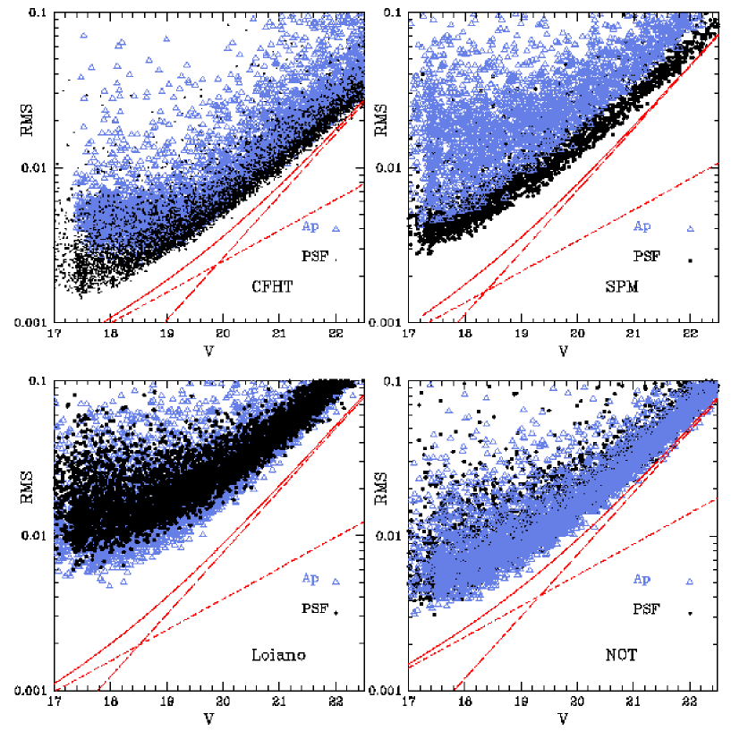
Figure 1: Comparison of the photometric precision for aperture photometry with neighbor subtraction (Ap) and for PSF fitting photometry (PSF) as a function of the apparent visual magnitude for CFHT, SPM, Loiano and NOT images. The short dashed line indicates the N/S considering only the star photon noise, the long dashed line is the N/S due to the sky photon noise and the detector noise. The continuous line is the total N/S.

It is clear that both the PSF fitting photometry and the aperture photometry tend to have larger errors with respect to the expected error level. This effect is much clearer for Loiano, SPM and NOT rather than for Hawaii photometry. As explained by Kjeldsen & Frandsen (kjeldsen92 (1992)), and more recently by Hartman et al. (hartman05 (2005)), the PSF fitting approach in general results in poorer photometry for the brightest sources with respect to the aperture photometry. But, for our data-sets, this was true only for the case of Loiano photometry, as demonstrated above. The aperture photometry routine in DAOPHOT returns for each star, along with other information, the modal sky value associated with that star, and the ${\emph{r}ms}$ dispersion ($\sigma_{\rm sky}$) of the sky values inside the sky annular region. So, we chose to calculate the error associated with the random noise inside the star’s aperture with the formula:

$$\sigma_{\rm Aperture}=\sqrt{\sigma_{\rm sky}^{2}\,{\rm Area}}$$ (3)

where Area is the area (in pixels²) of the region inside which we measure the star’s brightness. This error automatically takes into account the sky Poissonian noise, instrumental effects like the Read Out Noise, (RON), or detector non-linearities, and possible contributions of neighbor stars. To calculate this error, we chose a representative mean-seeing image, and subdivide the magnitude range in the interval $17.5\,<\,V\,<\,22.0$ into nine bins of 0.5 mag. Inside each of these bins, we took the minimum value of the stars’ sky variance as representative of the sky variance of the best stars in that magnitude bin. We over-plot this contribution in Fig. 4 which is relative to the San Pedro photometry. This error completely accounts for the observed photometric precision. So, the variance inside the star’s aperture is much larger than what is expected from simple photon noise calculations. This can be the effect of neighbor stars or of instrumental problems. For CFHT photometry, as we have good seeing conditions and an optimal telescope scale, crowding plays a less important role. Concerning the other sites, we noted that for Loiano the crowding is larger than for SPM and NOT, and this could explain the lower photometric precision of Loiano observations, along with the smaller telescope diameter. For NOT photometry, instead, the crowding should be larger than for San Pedro (since the scale of the telescope is larger) while the median seeing conditions are comparable for the two data-sets, as shown in Sect 2. Therefore this effect should be more evident for NOT rather than for SPM, but this is not the case, at least for what concerns aperture photometry. For PSF photometry, as it is seen in Fig. 2, the NOT photometric precision appears more scattered than the SPM photometry.

We are forced to conclude that poor flat fielding, optical distortions, non-linearity of the detectors and/or presence of saturated pixels in the brightest stars must have played a significant role in setting the aperture and PSF fitting photometric precisions.

4.2 PSF photometry against image subtraction photometry

Applying the image subtraction technique we were able to improve the photometric precision with respect to that obtained by means of the aperture photometry and the PSF fitting techniques. This appears evident in Fig. 2, in which the image subtraction technique is compared to the PSF fitting technique. Again, the best overall photometry was obtained for the $CFHT$, for the reasons explained in the previous subsection. For the image subtraction reduction, the photometric precision overcame the $0.001$ mag level for the brightest stars in the $CFHT$ data-set, and for the other sites it was around $0.002$ mag (for the $NOT$) or better (for $SPM$ and $Loiano$). This clearly allowed the search for planets in all these different data-sets. In this case, it was possible to include also the Loiano observations (up to $2$ magnitudes below the turn-off), and, for the other sites, to extend by about $0.5$-$1$ mag, the range of magnitudes over which the search for transits was possible, (see previous Section).

The reason for which image subtraction gave better results could be that it is more suitable for crowded regions (as the center of the cluster), because it doesn’t need isolated stars in order to calculte the convolution kernel while the subtraction of stars by means of PSF fitting can give rise to higher residuals, because it’s much more difficult to obtain a reliable PSF from crowded stars.

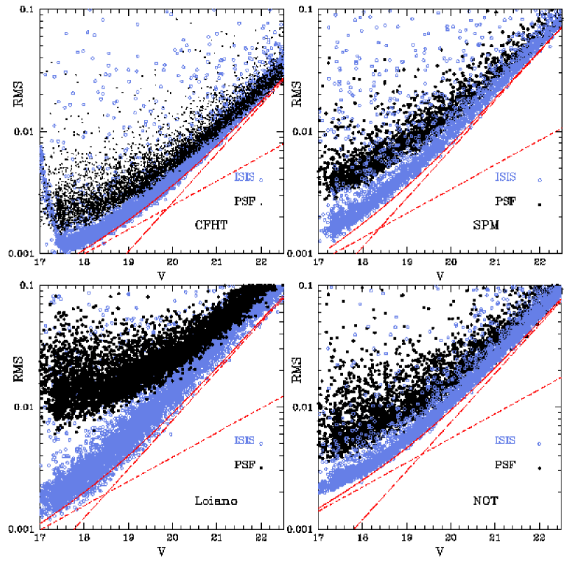
Figure 2: Comparison of the photometric precision for image subtraction (ISIS) and for psf fitting photometry (PSF) as function of the apparent visual magnitude for CFHT, SPM, Loiano, and NOT images.

4.3 The best photometric precision

Given the results of the previous comparisons, we decided to adopt the photometric data set obtained with the image subtraction technique. Figure 3, shows the photometric precision that we obtained for the four different sites. The photometric precision is very close to the theoretical noise for all the data-sets. The NOT data-set has a lower photometric precision with respect to SPM and even to Loiano, in particular for the brightest stars. We observed that the mean $S/N$ for the NOT images is lower than for the other sites because of the larger number of images taken (and consequently of their lower exposure times and $S/N$), see Tab. 1.

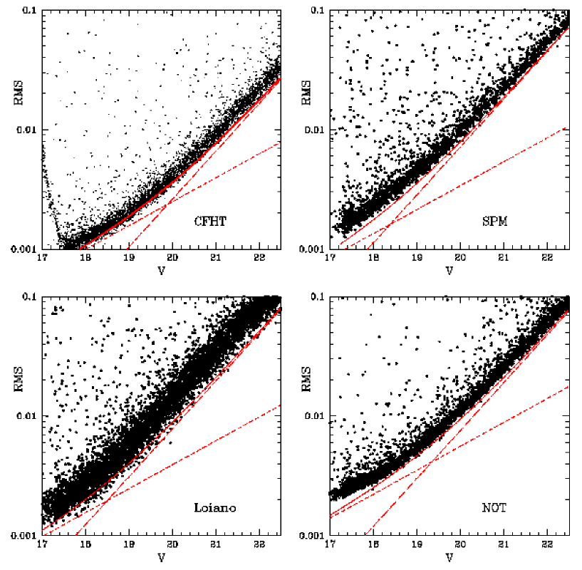
Figure 3: The expected RMS noise for the observations taken at the different sites as a function of the visual apparent magnitude, is compared with the RMS of the observed light curves obtained with the image subtraction technique.

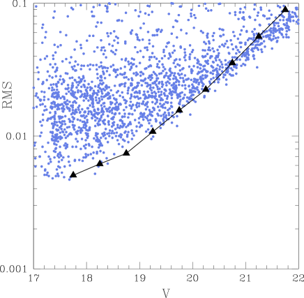
Figure 4: RMS noise for the San Pedro Mártir observations with the aperture error (triangles) as estimated by Equation 3.

5 Selection of cluster members

To detect planetary transits in NGC~6791 we selected the probable main sequence cluster members as follows. Calibrated magnitudes and colors were obtained by cross-correlating our photometry with the photometry by Stetson et al. (stetson03 (2003)), based on the same NOT data-set used in the present paper. Then, as done in M05, we considered $24$ bins of $0.2$ magnitudes in the interval $17.3\,<\,V\,<\,22.1$. For each bin, we calculated a robust mean of all (B-V) star colors, discarding outliers with colors differing by more than $\sim 0.06$ mag from the mean. Our selected main sequence members are shown in Fig. 5. Overall, we selected $3311$ main-sequence candidates in NGC~6791. These are the stars present in at least one of the four data-sets (see Sec. 8), and represent the candidates for our planetary transits search.

Note that our selection criteria excludes stars in the binary sequence of the cluster. These are blended objects, for which any transit signature should be diluted by the light of the unresolved companion(s) and then likely undetectable. Furthermore, a narrow selection range helps in reducing the field-star contamination.

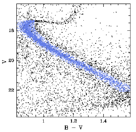
Figure 5: The NGC~6791 CMD highlighting the selection region of the main sequence stars (blue circles).

6 Description of the transit detection technique

6.1 The box fitting technique

To detect transits in our light curves we adopted the BLS algorithm by Kovács et al. (kovacs02 (2002)). This technique is based on the fitting of a box shaped transit model to the data. It assumes that the value of the magnitude outside the transit region is constant. It is applied to the phase folded light curve of each star spanning a range of possible orbital periods for the transiting object, (see Table 4). Chi-squared minimization is used to obtain the best model solution. The quantity to be maximized in order to get the best solution is:

$$T=\Big{(}\sum_{n=in}m_{n}\Big{)}^{2}\Big{[}\frac{1}{N_{in}\,N_{out}}\Big{]}$$ (4)

where $m_{n}=M_{n}\,-\,<M>$. $M_{n}$ is the $n$-th measurement of the stellar magnitude in the light curve, $<M>$ is the mean magnitude of the star and thus $m_{n}$ is the n-th residual of the stellar magnitude. The sum at the numerator includes all photometric measurements that fall inside the transit region. Finally $N_{in}$ and $N_{out}$ are respectively the number of photometric measurements inside and outside the transit region.

The algorithm, at first, folds the light curve assuming a particular period. Then, it sub-divides the folded light curve in $nb$ bins and starting from each one of these bins calculates the $T$ index shown above spanning a range of transit lengths between $qmi$ and $qma$ fraction of the assumed period. Then, it provides the period, the depth of the brightness variation, $\delta$, the transit length, and the initial and final bins in the folded light curve at which the maximum value of the index $T$ occurs. We used a routine called ’eebls’ available on the web. We applied also the so called directional correction (Tingley 2003a , 2003b ) which consists in taking into account the sign of the numerator in the above formula in order to retain only the brightness variations which imply a positive increment in apparent magnitude.

6.2 Algorithm parameters

The parameters to be set before running the BLS algorithm are the following: 1) nf, number of frequency points for which the spectrum is computed; 2) fmin, minimum frequency; 3) df, frequency step; 4) nb, number of bins in the folded time series at any test frequency; 5) qmi, minimum fractional transit length to be tested; 6) qma, maximum fractional transit length to be tested; $qmi$ and $qma$ are given as the product of the transit length to the test frequency. Table 4 displays our adopted parameters.

Table 4: Adopted parameters for the BLS algorithm: nf is the number of frequency steps adopted, fmin is the minimum frequency considered, df is the increasing frequency step, nb is the number of bins in the folded time series at any test frequency, qmi and qma are the minimum and maximum fractional transit length to be tested, as explained in the text.

nf	fmin(days-1)	df(days-1)	nb	qmi	qma
3000	0.1	0.0005	1000	0.01	0.1

6.3 Algorithm transit detection criteria

To characterize the statistical significance of a transit-like event detected by the BLS algorithm we followed the methods by Kovács & Bakos (kovacs05 (2005)): deriving the Dip Significance Parameter (hereafter DSP) and the significance of the main period signal in the Out of Transit Variation (hereafter OOTV, given by the folded time series with the exclusion of the transit).

The Dip Significance Parameter is defined as

$${\rm DSP}=\delta(\sigma^{2}/N_{\rm tr}+A^{2}_{\rm OOTV})^{-\frac{1}{2}}$$ (5)

where $\delta$ is the depth of the transit given by the BLS at the point at which the index $T$ is maximum, $\sigma$ is the standard deviation of the $N_{\rm tr}$ in-transit data points, $A_{\rm OOTV}$ is the peak amplitude in the Fourier spectrum of the Out of Transit Variation. The threshold for the DSP set by Kovacs & Bakos (kovacs05 (2005)) is $6.0$ and it was set on artificial constant light curves with gaussian noise. In real light curves the noise is not gaussian, as explained in Sec. 3.6, and, in general, the value of the DSP threshold should be set case by case. In Sec. 8, we presented the adopted thresholds, based on our simulations on artificial light curves, described in Sec. 7.

The significance of the main periodic signal in the OOTV is defined as:

$${\rm SNR}_{\rm OOTV}=\sigma_{A}^{-1}(A_{\rm OOTV}-<A>)$$ (6)

where $<A>$ and $\sigma_{A}$ are the average and the standard deviation of the Fourier spectrum. This parameter accounts for the Out Of Transit Variation, and we impose it to be lower than $7.0$, as in Kovacs & Bakos (kovacs05 (2005)).

For our search we imposed a maximum transit duration of six hours; we also required that at least ten data points must be included in the transit region.

7 Simulations

The Transit Detection Efficiency (TDE) of the adopted algorithm and its False Alarm Rate (FAR) were determined by means of detailed simulations. The TDE is a measure of the probability that an algorithm correctly identifies a transit in a light curve. The FAR is a measure of the probability that an algorithm identifies a feature in a light curve that does not represent a transit, but rather a spurious photometric effect.

In the following discussion, we address the details of the simulations we performed, considering the case of the CFHT observations of NGC~6791. Because the CFHT data provided the best of our photometric sequences, the results on the algorithm performance is shown below, and should be considered as an upper limit for the other cases.

7.1 Simulations with constant light curves

Artificial stars with constant magnitude were added to each image, according to an equally-spaced grid of 2*PSFRADIUS+1, (where the PSFRADIUS was the region over which the Point Spread Function of the stars was calculated, and was around $15$ pixels for the CFHT images), as described in Piotto & Zoccali (zoccali (1999)). We took into account the photometric zero-point differences among the images, and the coordinate transformations from one image to another. $7722$ stars were added on the CFHT images. In order to assure the homogeneity of these simulations, the artificial stars were added exactly in the same positions, (relative to the real stars in the field), for the other sites. Because of the different field of views of the detectors, (see Tab. 1), the number of resulting added stars was $3660$ for the NOT, $5544$ for Loiano, and $3938$ for SPM. The entire set of images was then reduced again with the procedure described in Sec.3. This way we got a set of constant light curves which is completely representative of many of the spurious artifacts that could have been introduced by the photometry procedure. This is certainly a more realistic test than simply considering Poisson noise on the light curves, as it is usually done. We then applied the algorithm, with the parameters described in Sec.6, to the constant light curves. The result is shown in Figure 6, where the DSP parameter is plotted against the mean magnitude of the light curve. For the CFHT data, fixing the DSP threshold at 4.3 yielded a FAR of $0.1\%$. This was the FAR we adopted also when considering the other sites, which corresponded to different levels of the DSP parameter, as explained in Sec. 8.

Repeating the whole procedure $4$ times and slightly shifting the positions of the artificial stars, allowed us to better estimate the FAR and its error, FAR=$(0.10\pm 0.04)\%$. Therefore, running the transit search procedure on the $3311$ selected main sequence stars, we expect $(3.3\,\pm\,1.3)$ false candidates.

Figure 6: False Alarm Probability (FAR) in %, against the DSP parameter given by the algorithm. The points indicate the results of our simulations on constant light curves, the solid line is our assumed best fit.

7.2 Masking bad regions and temporal intervals

We verified that, when stars were located near detector defects, like bad columns, saturate stars, etc., or, in correspondence of some instants of a particular night, (associated with sudden climatic variations, or telescope shifts), it was possible to have an over-production of spurious transit candidates. To avoid these effects, we chose to mask those regions of the detectors and the epochs which caused sudden changes in the photometric quality. This was done also for the simulations with the constant added stars, that were not inserted in detector defected regions, and in the excluded images that generating bad photometry. In particular, we observed these spurious effects for the NOT and SPM images. We further observed, when discussing the candidates coming from the analysis of the whole data-set (as described in Sec.10.3) that the photometric variations were concentrated on the first night of the NOT. This fact, which appeared from the simulations with the constant stars too, meant that this night was probably subject to bad weather conditions. had not we applied the Because we didn’t recognize it at the beginning, we retained that night, as long as those candidates, which were all recognized of spurious nature. Had not we applied any masking the number of false alarms would have almost quadruplicated. This fact probably can explain at least some of the candidates found by B03 (see Sec. 13) that were identified on the NOT observations. Even if some kind of masking procedure was applied by B03, many candidates appeared concentrated on the same dates, and were considered rather suspicious by the same authors.

7.3 Artificially added transits

The transit detection efficiency (TDE) was determined by analyzing light curves modified with the inclusion of random transits. To properly measure the TDE and to estimate the number of transits we expect to detect it is mandatory to consider realistic planetary transits. We proceeded as follows:

7.3.1 Stellar parameters

The basic cluster parameters were determined by fitting theoretical isochrones from Girardi et al. (girardi02 (2002)) to the observed color-magnitude diagram (Stetson et al. stetson03 (2003)). Our best fit parameters are (see Fig. 7): age = 10.0 Gyr, $(m-M)=13.30$, $E_{\rm(B-V)}=0.12$ for $Z=0.030$ (corresponding to [Fe/H]$=+0.18$), and age = 8.9 Gyr, $(m-M)=13.35$ and $E_{\rm(B-V)}=0.09$ for Z=0.046 (corresponding to [Fe/H]$=+0.39$).

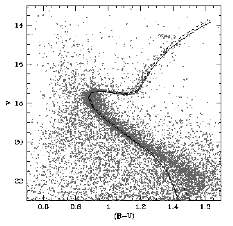
Figure 7: CMD diagram of NGC6791 with the best fit Z=0.030 isochrone (dashed line), and the best fit Z=0.046 isochrone (from Carraro et al. carraro06 (2006), solid line). Photometry: Stetson et al. (stetson03 (2003))

From the best-fit isochrones we then obtained the values of stellar mass and radius as a function of the visual magnitude (Fig. 8).

Figure 8: Left: $M_{i}/M_{\odot}$ vs visual apparent magnitude Right: $R_{i}/R_{\odot}$ vs visual apparent magnitude, from our best fit isochrone (dashed line) and from the Z=0.046 isochrone (solid line) applied to the stars of NGC~6791.

7.3.2 Planetary parameters

The actual distribution of planetary radii has a very strong impact on the transit depth and therefore on the number of planetary transits we expect to be able to detect. The radius of the fourteen transiting planets discovered to date ranges from R=$1.35\,\pm\,0.07\,R_{J}$ (HD209458b; Wittenmyrer et al. wittenmyer05 (2005)) to R=$0.725\,\pm\,0.03\,R_{J}$ (HD149026b; Sato et al. sato05 (2005)), where $J$ refers to the value for Jupiter. The observed distribution is likely biased towards larger radii. Gaudi (2005a) suggests for the close-in giant planets a mean radius $R_{p}=1.03\leavevmode\nobreak\ \,\leavevmode\nobreak\ R_{J}$. To evaluate the efficiency of the algorithm we have considered three cases:

• $R_{p}=(0.7\,\pm\,0.1)\,R_{J}$

• $R_{p}=(1.0\,\pm\,0.2)\,R_{J}$

• $R_{p}=(1.4\,\pm\,0.1)\,R_{J}$

assuming a Gaussian distribution for $R_{p}$. We fixed the planetary mass at $M_{p}=1\,M_{J}$, because the effect of planet mass on transit depth or duration is negligible.

The period distribution was taken from the data for planets discovered by radial velocity surveys, from the Extra-solar Planets Encyclopaedia. We selected the planets discovered by radial velocity surveys with mass $0.3M_{J}\leq M_{pl}\sin i\leq 10M_{J}$ (the upper limit was fixed to exclude brown dwarfs; the lower limit to ensure reasonable completeness of RV surveys and to exclude Hot Neptunes that might have radii much smaller than giant planets, Baraffe et al. baraffe05 (2005)) and periods $1\leq P\leq 9$ days. We assumed that the period distribution of RV planets is unbiased in this period range. We then fitted the observed period distribution with a positive power law for the Very Hot Jupiters (VHJ, $1\leq P\leq 3$) and a negative power law for the Hot Jupiters (HJ, $3<P\leq 9$, see Gaudi et al. 2005b for details) as shown in Fig. 9.

Figure 9: Continuous line: adopted distribution for planet periods. Histogram: RV surveys data (from the Extrasolar Planets Encyclopaedia).

7.3.3 Limb-darkening

To obtain realistic transit curves it is important to include the limb darkening effect. We adopted a non-linear law for the specific intensity of a star:

$$\frac{I(\mu)}{I(1)}=1-\sum_{k=1}^{4}\,a_{k}\,(1-\mu^{k/2})$$ (7)

from Claret (claret (2000)).

In this relation $\mu=\cos\gamma$ is the cosine of the angle between the normal to the stellar surface and the line of sight of the observer, and $a_{k}$ are numerical coefficients that depend upon $v_{turb}$ (micro-turbulent velocity), [M/H], $T_{eff}$, and the spectral band. The coefficients are available from the ATLAS calculations (available at CDS).

We adopted the metallicity of the cluster for [M/H] and $v_{turb}$=2 km s^-1 for all the stars. For each star we adopted the appropriate $V$-band $a_{k}$ coefficients as a function of the values of $\log g$ and $T_{eff}$ derived from the best fit isochrone.

7.3.4 Modified light curves

In order to establish the TDE of the algorithm, we considered the whole sample of constant stars with $17.3\leq V\leq 22.1$, and each star was assigned a planet with mass, radius and period randomly selected from the distributions described above. The orbital semi-major axis $a$ was derived from the $3^{rd}$ Kepler’s law, assuming circular orbits.

To each planet, we also assigned an orbit with a random inclination angle $i$, with $0<\cos i<0.1$, with a uniform distribution in $\cos i$. We infer that $\sim 85\%$ of the planets result in potentially detectable transits. We also assigned a phase $2\phi_{0}$ randomly chosen from $0$ to $2\pi$ rad and a random direction of revolution $s=\pm 1$ (clockwise or counter-clockwise).

Having fixed the planet’s parameters ($P$, $i$, $\phi_{0}$, $M_{p}$, $R_{p}$, $a$), the star’s parameters ($M_{\star}$, $R_{\star}$) and a constant light curve ($t_{i}$ , $V_{i}$) it is now possible to derive the position of the planet with respect to the star at every instant from the relation:

$$\phi=\phi_{0}+\frac{2\pi s}{P}t_{i}$$

where $\phi$ is the angle between the star-planet radius and the line of sight. The positions were calculated at all times $t_{i}$ corresponding to the $V_{i}$ values of the light curve of the star. When the planet was transiting the star, the light curve was modified, calculating the brightness variation $\Delta V(t_{i})$ and adding this value to the $V_{i}$ (see Fig. 10).

Figure 10: Top: constant light curve Bottom: the same light curve after inserting the simulated transit with limb-darkening (black points). The solid line shows the theoretical light curve of the transit.

7.4 Calculating the TDE

We then selected only the light curves for which there was at least a half transit inside an observing night and applied our transit detection algorithm. We considered not only central transits but also grazing ones. We considered the number of light curves that exceeded the thresholds, and also determined for how many of these the transit instants were correctly identified on the unfolded light curves.

We isolated three different outputs:

1. Missed candidates: the light curves for which the algorithm did not get the values of the parameters that exceeded the thresholds (DSP, OOTV, transit duration and number of in transit points, see Sec 6.3), or if it did, the epochs of the transits were not correctly recovered;

2. Partially recovered transit candidates: the parameters exceeded the thresholds and at least one of the transits that fell in the observing window was correctly identified;

3. Totally recovered transit candidates: the parameters exceeded the thresholds and all the transits that were present were correctly recovered.

The TDE was calculated as the sum of the totally and partially recovered transit candidates relative to the whole number of stars with transiting planets. We derive the TDE as a function of magnitude in Fig. 11. The TDE decreases with increasing magnitude because the lower photometric precision at fainter magnitudes is not fully compensated by the larger transit depth. The TDE depends strongly also on the assumptions concerning the planetary radii, and on the inclusion of the limb darkening effect. Fig. 11 is relative to a threshold equal to $4.3$ for the DSP (cf. Fig. 6).

The resulting TDE is about $11.5\%$ around $V=18$ and $1\%$ around $V=21$ for the case with $R=(1.0\,\pm\,0.2)R_{J}$.

Figure 12–14 show the histograms relative to the input transit parameters and the recovered values of the BLS algorithm normalized to the whole number of transiting planets. For comparison we also show in the upper left panel of each figure the recovered values of the BLS for the constant simulated light curves (normalized to the total number of constant light curves). We found that on average the BLS algorithm has underestimated the depth and duration of the transit by about 15-20%. This is likely due to the deviation of the transit curves from the box shape assumed by the algorithm. For the periods, (Fig. 13), the recovered transit period distribution shown in the upper right panel of Fig. 13, had two clear peaks at $1.5$ and $3$ days, with the first one much more evident meaning that the algorithm tends to estimate half of the input transit period, as shown in the lower panels of the same Figure. The constant light curve period distribution of the upper left panel, instead, showed that the vast majority of constant stars were recovered with periods between $0.5$ and $1$ day, but residual peaks at $2.5$ and $5$ days were present.

Figure 11: TDE as a function of the stellar magnitude for various assumptions on planetary radii distribution. From the top to the bottom: 1) Dashed line, $R=(1.4\,\pm\,0.1)\,R_{J}$; 2) Solid line, $R=(1.0\,\pm\,0.2)\,R_{J}$; 3) Dotted line, $R=(0.7\,\pm\,0.1)\,R_{J}$. The adopted threshold for the DSP in this figure is $4.3$. The normalization is respect to the whole number of transiting planets.

Figure 12: (Upper left) Distributions of transit depths measured by the BLS algorithm on the artificial constant-light-curves (lc); (upper right) transit depths measured on artificial light curves with transits added;(lower left) input transit depths used to generate artificial light curves with transits;(lower right) relative difference between the transit depth recovered by BLS and its input value. Empty histograms refer to distributions relative to all light curves, filled ones to light curves with totally and partially recovered transits. Histograms are normalized to all light curves with transiting planets, or, for the upper left panel to all constant light curves. This Figure is relative to CFHT data, and the assumed planetary radii distribution is $R=(1.0\,\pm\,0.2)$.

Figure 13: The same as Fig.12 for the transit periods.

Figure 14: The same as Fig.12 for the transit durations.

8 Different approaches in the transit search

The data we have acquired on NGC~6791 came from four different sites and involved telescopes with different diameters and instrumentations. Moreover, the observing window of each site was clearly different with respect to the others as well as observing conditions like seeing, exposure times, etc.

The first approach we tried consisted in putting together the observations coming from all the different telescopes. The most important complication we had to face regarded the different field of views of the detectors. This had the consequence that some stars were measured only in a subset of the sites, and therefore these stars had in general different observing windows. Considering only the stars in common would reduce the number of candidates from $3311$ to $1093$ which means a reduction of about $60\%$ of the targets. We decided to distinguish eight different cases, which are shown in Tab. 5. In the first column a simple binary notation identifies the different sites: each digit represents one site in the following order: CFHT, SPM, Loiano, NOT(V) and NOT(I). If the number correspondent to a generic site is $1$, it indicates that the stars contained in that case have been observed, otherwise the value is set to $0$. For example, the notation $11111$ was used for the stars in common to all 4 sites. The notation $10000$ indicates the number of stars which were present only on the CFHT field, and so on. Each one of these cases was treated as independent, and the resulting FAR and expected number of transiting planets were added together in order to obtain the final values.

The second approach we followed was to consider only the CFHT data. As demonstrated in Section 3, overall we obtained the best photometric precision for this data-set. We considered the $3311$ candidates which were recovered in the CFHT data-set.

For the CFHT data-set, as shown in Tab. 5, the DSP value correspondent to a FAR$=0.1\%$ is equal to $4.3$, lower than the other cases reported in that Table. Thus, despite the reduced observing window of the CFHT data, it is possible to take advantage of its increased photometric precision in the search for planets.

In Section 9, and in Section 10, we presented the candidates and the different expected number of transiting planets for these two different approaches.

Table 5: The different cases in which the data-sets analysis was splitted into. The notation in the first column is explained in the text, the second column shows the number of stars in each case and the third column refers to the DSP values assumed, correspondent to a FAR$=0.1\%$.

Case	N.stars	DSP threshold
$11111$	$1093$	7.5
$10000$	$771$	4.3
$10100$	$870$	5.5
$11011$	$162$	7.1
$10001$	$112$	7.1
$11001$	$108$	7.5
$10111$	$99$	7.2
$10011$	$96$	6.5

9 Presentation of the candidates

Table 6 shows the characteristics of the candidates found by the algorithm, distinguishing those coming from the entire data-set analysis from those coming from the CFHT analysis.

Table 6: The candidates found in the two cases discussed in Sec. 8. The case of the whole data-sets put together is indicated with $ALL$ ($1^{st}$ column), that one for the $only$ CFHT data-set is indicated with $CFHT$ ($2^{nd}$ column). A cross (x) indicates that the candidate was found in that case, a trait (-) that it is absent. In the $3^{rd}$ column, the $ID$ of the stars taken from S03 is shown. Follow the $V$ calibrated magnitude, the $(B-V)$ color, the right ascension, ($\alpha$), and the declination, ($\delta$), of the stars.

$ALL$	$CFHT$	$ID(Stetson)$	$V$	$(B-V)$	$\alpha(2000)$	$\delta(2000)$
x	-	$6598$	$18.176$	$0.921$	$19^{h}$ $20^{m}$ $48^{s}.65$	$+37^{\circ}$ $47^{{}^{\prime}}$ $41.^{{}^{\prime\prime}}1$
x	-	$4304$	$17.795$	$0.874$	$19^{h}$ $20^{m}$ $41^{s}.39$	$+37^{\circ}$ $43^{{}^{\prime}}$ $28.^{{}^{\prime\prime}}9$
x	-	$4699$	$17.955$	$0.846$	$19^{h}$ $20^{m}$ $42^{s}.67$	$+37^{\circ}$ $43^{{}^{\prime}}$ $31.^{{}^{\prime\prime}}5$
x	x	$1239$	$19.241$	$1.058$	$19^{h}$ $20^{m}$ $25^{s}.42$	$+37^{\circ}$ $47^{{}^{\prime}}$ $45.^{{}^{\prime\prime}}2$
-	x	$4300$	$18.665$	$0.697$	$19^{h}$ $20^{m}$ $41^{s}.38$	$+37^{\circ}$ $45^{{}^{\prime}}$ $23.^{{}^{\prime\prime}}3$
-	x	$7591$	$18.553$	$0.959$	$19^{h}$ $20^{m}$ $51^{s}.51$	$+37^{\circ}$ $48^{{}^{\prime}}$ $58.^{{}^{\prime\prime}}7$

9.1 Candidates from the whole data-sets

Applying the algorithm with the DSP thresholds shown in Tab. 5 on the real light curves we obtained four candidates. Hereafter we adopt the S03 notation reported in Tab. 6. For what concerns candidates $6598$, $4304$, and $4699$ (Fig. 15, 16, 17) we noted (see also Sec. 7.2) that the points contributing to the detected signal came from the first observing night at the NOT, meaning that bad weather conditions deeply affected the photometry during that night. In particular candidate $6598$, was also found in the B03 transit search survey, (see Sec. 13), and flagged as a probable spurious candidate. In none of the other observing nights we were able to confirm the photometric variations which are visible in the first night at the NOT. We concluded that these three candidates are of spurious nature.

The fourth candidate corresponds to star $1239$, that is located in the external regions of the cluster. For this reason we presented in Fig. 18 only the data coming from the CFHT. In this case, the data points appear irregularly scattered underlying a particular pattern of variability or simply a spurious photometric effect.

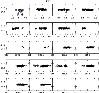
Figure 15: Composite light curve of candidate $6598$. In ordinate is reported the calibrated V magnitude and in abscissa the observing epoch, (in days), where $0$ corresponds to $JD=52099$. Filled circles indicate CFHT data, crosses SPM data, open triangles Loiano data, open circles NOT data in the V filter and open squares NOT data in the I filter. Light blue symbols highlight regions which were flagged by the BLS.

Figure 16: Composite light curve of candidate $4304$.

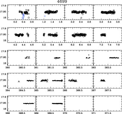
Figure 17: Composite light curve of candidate $4699$.

9.2 Candidates from the CFHT data-set

Considering only the data coming from the CFHT observing run we obtained three candidates. The star $1239$ is in common with the list of candidates coming from the whole data-sets because, as explained above, it is located in the external regions for which we had only the CFHT data. For candidate $4300$, the algorithm identified two slight ($\sim\,0.004\,$ mag) magnitude variations with duration of around one hour during the sixth and the tenth night, with a period of around $4.1$ days. A jovian planet around a main sequence star of magnitude V=$18.665$, (with $R=0.9\,R_{\odot}$, see Fig. 8), should determine a transit with a maximum depth of around $1.2\%$, and maximum duration of $2.6$ hours. Although compatible with a grazing transit, we observed that the two suspected eclipses are not identical, and, in any case, outside these regions, the photometry appears quite scattered. Star $7591$, instead, does not show any significant feature.

From the analysis of these candidates we concluded that no transit features are detected for both the entire data-sets and the CFHT data. Moreover, we can say to have recovered the expected number of false alarm candidates which was $(3.3\,\pm\,1.3)$ as explained in Sec. 10.3.

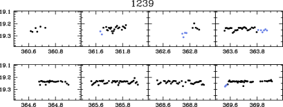
Figure 18: CFHT light curve for candidate $1239$.

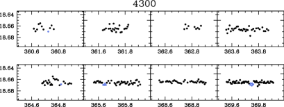
Figure 19: CFHT light curve for candidate $4300$.

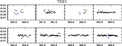
Figure 20: CFHT light curve for candidate $7591$.

10 Expected number of transiting planets

10.1 Expected frequency of close-in planets in NGC~6791

The frequency of short-period planets in NGC~6791 was estimated considering the enhanced occurrence of giant planets around metal rich stars and the fraction of hot Jupiters among known extrasolar planets.

Fischer & Valenti (fischer05 (2005)) derived the probability $\mathcal{P}$ of formation of giant planets with orbital period shorter than 4 yr and radial velocity semi-amplitude $K>30$ ms^-1 as a function of [Fe/H]:

$$\mathcal{P}=0.03\cdot 10^{\,2.0\,{\rm[Fe/H]}}\hskip 28.45274pt-0.5<{\rm[Fe/H]}<0.5$$ (8)

The number of stars with a giant planet with $P<9$ d was estimated considering the ratio between the number of the planets with $P<9$ days and the total number of planets from Table 3 of Fischer & Valenti fischer05 (2005) (850 stars with uniform planet detectability). The result is $0.22^{+0.12}_{-0.09}$.

Assuming for NGC~6791 [Fe/H]$=+0.17$ dex, a conservative lower limit to the cluster metallicity, from Equation 8 we determined that the probability that a cluster star has a giant planet with $P<9$ is 1.4%. Assuming [Fe/H]$=+0.47$, the metallicity resulting from the spectral analysis by Gratton et al. (gratton06 (2006)), the probability rises to 5.7%.

Our estimate assumes that the planet period and the metallicity of the parent star are independent, as found by Fischer & Valenti (fischer05 (2005)). If the hosts of hot Jupiters are even more metal rich than the hosts of planets with longer periods, as proposed by Society (sozzetti04 (2004)), then the expected frequency of close-in planets at the metallicity of NGC~6791 should be slightly higher than our estimate.

10.2 Expected number of transiting planets

In order to evaluate the expected number of transiting planets in our survey we followed this procedure:

• From the constant stars of our simulations (see Sec. 7), taking into account the luminosity function of main sequence stars of the cluster, we randomly selected a sample corresponding to the probability that a star has a planet with $\rm P\leq 9$ d.

• From the $V$ magnitude of the star we calculated the mass and radius.

• To each star in this sample we assigned a planet with mass, radius, period randomly chosen from the distributions described in Sec. 7.3.2, and $cos\,i$ randomly chosen inside the range $0\,$-$\,1$. The range spanned for the periods was $\rm 1\,<\,P\,<\,9$ days, with a step size of $0.006$ days. For planetary radii we considered the three distributions described in Sec. 7.3.2, sampled with a step size of $\rm 0.001\,R_{J}$, and inclinations were varied of $0.005$ degrees.

• We selected only the stars with planets that can make transits thanks to their inclination angle given by the relation:

  $$\rm\cos i\leq\frac{R_{pl}+R_{\star}}{a}$$

• Finally, as described above, we assigned to each planet the initial phase $\phi_{0}$ and the revolution orbital direction $s$ and modified the constant light curves inserting the transits. The initial phase was chosen randomly inside the range $0$-$360$ degrees, with a step size of $0.3$ degrees.

• We applied the BLS algorithm to the modified light curves with the adopted thresholds.

  We performed $7000$ different simulations and we calculated the mean values of these quantities:

  • The number of MS stars with a planet: $N_{pl}$

  • The number of planets that make transits (thanks to their inclination angles): $N_{geom}$

  • The number of planets that make one or more transits in the observing window: $N_{+1}$

  • The number of planets that make one single transit in the observing window: $N_{1}$

  • The number of transiting planets detected by the algorithm for the three different planetary radii distributions adopted, (as described in Sect. 7), $R^{1}=(0.7\,\pm\,0.1)\,R_{J}$, $R^{2}=(1.0\,\pm\,0.2)\,R_{J}$, and $R^{3}=(1.4\,\pm\,0.1)\,R_{J}$.

10.3 FAR and expected number of detectable transiting planets for the whole data-sets

We followed the procedure reported in Sec. 7 to perform simulations with the artificial stars. It is important to note that artificial stars were added exactly in the same positions in the fields of the different detectors. This is important because it assured the homogeneity of the artificial star tests. We decided to accept a FAR equal to $0.1\%$, which meant that we expected to obtain $(3.3\,\pm\,1.3)$ false alarms from the total number of $3311$ cluster candidates. The DSP thresholds correspondent to this FAR value are different for each case, and is reported in Table 5.

Table 7 displays the results for the simulations performed in order to obtain the expected numbers of detectable transiting candidates for three values of [Fe/H] (the values found by Carraro et al. carraro06 (2006) and Gratton et al. gratton06 (2006) and a conservative lower limit to the cluster metallicity).

The columns listed as $N_{geom}$, $N_{1+}$ and $N_{1}$ indicate respectively the number of planets which have a favorable geometric inclination for the transit, the number of expected planets that transit at least one time within the observing window and the number of expected planets that transit exactly one time in the observing window.

The numbers of expected transiting planets in our observing window detectable by the algorithm were calculated for the three different planetary radii distributions (see Sec. 7, and previous paragraph). On the basis of the current knowledge on giant planets the most likely case corresponds to $R^{2}=(1.0\,\pm\,0.2)\,R_{J}$.

Table 7 shows that, assuming the most likely planetary radii distribution $R=(1.0\,\pm\,0.2)\,R_{J}$ and the high metallicity resulting from recent high dispersion studies (Carraro et al. carraro06 (2006); Gratton et al. gratton06 (2006)), we expected to be able to detect $2-3$ planets that exhibit at least one detectable transit in our observing window.

Table 7: The Table shows the results of our simulations on the expected number of detectable transiting planets for the whole data-set (all the cases of Tab. 5) as explained in Sect. 10.3. $N_{geom}$ indicates planets with favorable inclination for transits, $N_{1+}$, and $N_{1}$, planets that transit respectively at least one time and only one time inside the observing window. $R^{1}$, $R^{2}$, $R^{3}$, indicate the expected number of detectable transiting planets inside our observing window, for the three assumed planetary radii distributions, (see Sec. 7.3.2).

[Fe/H]	$N_{geom}$	$N_{1+}$	$N_{1}$	$R^{1}$	$R^{2}$	$R^{3}$
+0.17	5.39	3.08	1.68	$\bf 0.0\,\pm\,0.0$	$\bf 0.0\,\pm\,0.0$	$\bf 1.8\,\pm\,0.9$
+0.39	15.13	8.32	4.60	$\bf 0.1\,\pm\,0.1$	$\bf 1.9\,\pm\,0.8$	$\bf 3.6\,\pm\,1.8$
+0.47	21.92	11.95	6.62	$\bf 0.2\,\pm\,0.3$	$\bf 3.2\,\pm\,1.9$	$\bf 5.4\,\pm\,1.8$

10.4 FAR and expected number of detectable transiting planets for the CFHT data-set

Table 8 shows the expected number of detectable planets in our observing window for the case of the $CFHT$ data. A comparison with Table 7 revealed that, in general, except for the largest planetary radii distribution, $R^{3}$, the number of expected detections is not increasing considering all the sites together instead of the $CFH$ only. Moreover, for the cases of [Fe/H]$=(+0.39,+0.47)$dex, and the $R=(0.7\,\pm\,0.1)R_{J}$ radii distribution, we obtained significantly better results considering only the $CFHT$ data than putting together all the data-sets. We interpreted this result as the evidence that the transit signal is, in general, lower than the total scatter in the composite light curves and this didn’t allow the algorithm to take advantage of the increased observing window giving, for the cases of major interest, $R=(1\,\pm\,0.2)R_{J}$ and [Fe/H]$=(+0.39,+0.47)$dex, comparable results.

Table 8: The same as 7, but for the case of the only $CFHT$ data as explained in Sect. 10.2.

[Fe/H]	$N_{geom}$	$N_{1+}$	$N_{1}$	$R^{1}$	$R^{2}$	$R^{3}$
+0.17	5.39	2.49	1.98	$\bf 0.2\,\pm\,0.5$	$\bf 0.4\,\pm\,0.7$	$\bf 0.6\,\pm\,0.8$
+0.39	15.13	7.01	5.39	$\bf 1.6\,\pm\,1.3$	$\bf 2.3\,\pm\,1.6$	$\bf 2.6\,\pm\,1.7$
+0.47	21.92	10.12	7.94	$\bf 2.5\,\pm\,1.7$	$\bf 3.4\,\pm\,2.0$	$\bf 4.0\,\pm\,2.1$

11 Significance of the results

As explained in Sec. 9, on real data we obtained $4$ candidates, considering the data coming from the entire data-sets, (all the cases of Tab. 5), and $3$ candidates considering only the best photometry coming from the $CFHT$. None of these candidates shows clear transit features, and their number agrees with the expected number of false candidates coming from the simulations $(3.3\,\pm\,1.3)$ as explained in Sec. 7.1.

Considering the case relative to the metallicity of Carraro et al. carraro06 (2006) ([Fe/H]$=+0.39$) and the one relative to the metallicity of Gratton et al. gratton06 (2006), ([Fe/H]$=+0.47$), and given the most probable planetary radii distribution with $R=(1.0\,\pm\,0.2)R_{J}$, from Table 7 and Table 8 we expected between $2$ and $3$ planets with at least one detectable transit inside our observing window.

Therefore, this study reveals a lack of transit detections.

What is the probability that our survey resulted in no transiting planets just by chance? To answer this question we went back to the simulations described in Sect. 10.2 and calculated the ratio of the number of simulations for which we were not able to detect any planet relative to the total number of simulations performed. The resulting probabilities to obtain no transiting planets were respectively around $10\%$ and $3\%$ for the metallicities of Carraro et al. carraro06 (2006) and Gratton et al. gratton06 (2006) considered above.

12 Implication of the results

Beside the rather small, but not negligible probability of a chance result, ($3$-$10$%, see Sec. 11), different hypothesis can be invoked to explain the lack of observed transits. We have discussed them here.

12.1 Lower frequency of close-in planets in cluster environments

The lack of observed transits might be due to a lower frequency of close-in planets in clusters compared to the field stars of similar metallicity. In general, two possible factors could prevent planet formation especially in clustered environments:

• in the first million years of the cluster life, UV-flux can evaporate fragile embryonic dust disks from which planets are expected to form. Circumstellar disks associated with solar-type stars can be readily evaporated in sufficiently large clusters, whereas disks around smaller (M-type) stars can be evaporated in more common, smaller groups. In addition, even though giant planets could still form in the disk region $r\,=\,5$-$15$ AU, little disk mass (outside that region) would be available to drive planet migration.;

• on the other hand, gravitational forces could strip nascent planets from their parent stars or, taking in mind that transit planet searches are biased toward ’hot jupiter’ planets, tidal effects could prevent the planetary migration processes which are essential for the formation of this kind of planets.

These factors depend critically on the cluster size. Adams et al. (2006), show that for clusters with $100$-$1000$ members modest effects are expected on forming planetary systems. The interaction rates are low, so that the typical solar system experiences a single encounter with closest approach distance of $1000$ AU. The radiation exposure is also low, so that photo-evaporation of circumstellar disks is only important beyond $30$ AU. For more massive clusters like NGC6791, these factors are expected to be increasingly important and could drastically affect planetary formation (Adams et al. 2004).

12.2 Smaller planetary radii for planets around very metal rich host stars

Guillot et al. (2006) suggested that the masses of heavy elements in planets was proportional to the metallicities of their parent star. This correlation remains to be confirmed, being still consistent with a no-correlation hypothesis at the $1/3$ level in the least favorable case. A consequence of this would be a smaller radius for close-in planets orbiting super-metal rich stars. Since the transit depth scales with the square of the radius, this would have important implications for ground-based transit detectability, (see Tables 8- 7).

12.3 Limitations on the assumed hypothesis

While we exploited the best available results to estimate the expected number of transiting planets, it is possible that some of our assumptions are not completely realistic, or applicable to our sample. One possibility is that the planetary frequency no longer increases above a given metallicity. The small number of stars in the high metallicity range in the Fischer & Valenti sample makes the estimate of the expected planetary frequency for the most metallic stars quite uncertain. Furthermore, the consistency of the metallicity scales of Fischer & Valenti (2005), Carraro et al. (2006) and Gratton et al. (2006) should be checked.

Another possibility concerns systematic differences between the stellar sample studied by Fischer & Valenti, and the present one. One relevant point is represented by binary systems. The sample of Fischer & Valenti has some biases against binaries, in particular close binaries. As the frequency of planets in close binaries appears to be lower than that of planets orbiting single stars and wide binaries (Bonavita & Desidera 2007, A&A, submitted), the frequency of planets in the Fischer & Valenti sample should be larger than that resulting in an unbiased sample. On the other hand, our selection of cluster stars excludes the stars in the binary sequence, partially compensating this effect.

Another possible effect is that of stellar mass. As shown in Fig. 8, the cluster’s stars searched for transits have mass between $1.1$ to $0.5$ M_⊙. On the other hand, the stars in the FV sample have masses between $1.6$ to $0.8$ M_⊙. If the frequency of giant planets depends on stellar mass, the results by Fischer & Valenti (2005) might not be directly applicable to our sample.

Furthermore, some non-member contamination is certainly present. As discussed in Section 5, the selection of cluster members was done photometrically around a fiducial main sequence line.

12.4 Possibility of a null result being due to chance

As shown in Sec. 11, the probability that our null result was simply due to chance was comprised between $3$% and $10$%, depending on the metallicity assumed for the cluster. This is a rather small, but not negligible probability, and other efforts must be undertaken to reach a firmer conclusion.

13 Comparison of the transit search surveys on NGC~6791

It is important to compare our results on the presence of planets with those of other photometric campaigns performed in past years. We consider in this comparison B03 and M05.

13.1 The Nordic Optical Telescope (NOT) transit search

As already described in this paper, (e.g. see Sect. 2), in July $2001$, at NOT, B03 undertook a transit search on NGC~6791 that lasted eight nights. Only seven of these nights were good enough to search for planetary transits. Their time coverage was thus comparable to the CFHT data presented here. The expected number of transits was obtained considering as candidates all the stars with photometric precision lower than $2\%$, (they did not isolate cluster main sequence stars, as we did, but they then multiplied their resulting expected numbers for a factor equal to $85\%$ in order to account for binarity), and assuming that the probability that a local G or F-type field star harbors a close-in giant planet is around $0.7\%$. With these and other obvious assumptions B03 expected $0.8$ transits from their survey. However, they made also the hypothesis that for metal-rich stars the fraction of stars harboring planets is $\sim 10$ times greater than for general field stars, following Laughlin (laughlin00 (2000)). In this way, they would have expected to find “at least a few candidates with single transits”. In Section 3 we showed how the photometric precision for the NOT was in general of lower quality for the brightest stars with respect to that one of SPM and Loiano. This fact can be recognized also in Table 5 where the value of the threshold for the DSP was always bigger than $6.5$ when the NOT observations were included. This demonstrates the higher noise level of this data-set. We did not perform the accurate analysis of the expected number of transiting planets considering only the NOT data, but, on the basis of our assumptions, and on the photometric precision of the NOT data, the numbers showed in Table 8 for the CFHT should be considered as an upper limit for the expected transit from the NOT survey.

B03 reported ten transit events, two of which, (identified in B03 as T6 and T10), showed double transit features, and the others were single transits. Except for candidate T2, which was recovered also in our analysis (see Sec. 9.1) our algorithm did not identify any other of the candidates reported by B03.

B03 recognized that most of the candidates were likely spurious, while three cases, referred as T5, T7 and T8, were considered the most promising ones. We noted that T8 lies off the cluster main sequence. Therefore, it can not be considered as a planet candidate for NGC~6791. Furthermore, from our CFHT images we noted that this candidate is likely a blended star. The other two candidates were on the main sequence of NGC~6791. Visual inspection of the light curves in Fig. 21 and Fig. 22 also show no sign of eclipse.

Finally, candidate T9, (Fig. 23) lies off the cluster main sequence and it was recognized by B03 to be a long-period low-amplitude variable (V80). In our photometry, it shows clear signs of variability, and a $\sim 0.05$ mag eclipse during the second night of the CFHT campaign at $t=361.8$, and probably a partial eclipse at the end of the seventh night of the NOT data-set, at $t=6.4$, ruling out the possibility of a planetary transit, because the magnitude depth of the eclipse is much larger than what is expected for a planetary transit.

It is not surprising that almost all of the candidates reported by B03 were not confirmed in our work, even for the NOT photometry itself. Even if the photometry reduction algorithm was the same, (image subtraction, see Sec. 3), all the other steps that followed, and the selection criteria of the candidates were in general different. This, in turn, reinforces the idea that they are due to spurious photometric effects.

Figure 21: Composite light curve for candidate $3671$ correspondent to T5 of BO3. Different symbols have the same meaning of Fig. 15.

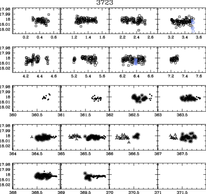
Figure 22: Composite light curve for candidate $3723$ correspondent to T7 of BO3.

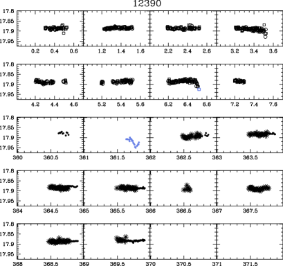
Figure 23: Composite light curve for candidate $12390$ correspondent to T9 of BO3.

13.2 The PISCES group extra-Solar planets search

The PISCES group collected $84$ nights of observations on NGC~6791, for a total of $\sim\,300$ hours of data collection from July $2001$ to July $2003$, at the $1.2$m Fred Lawrence Whipple Observatory (M05). Starting from their $3178$ cluster members (selected considering all the main sequence stars with RMS$\leq 5\%$), assuming a distribution of planetary radii between $0.95\,R_{J}$ and $1.5\,R_{J}$, and a planet frequency of $4.2\%$, M05 expected to detect $1.34$ transiting planets in the cluster. They didn’t identify any transiting candidate. Their planet frequency is within the range that we assumed ($1.4\%$–$5.7\%$). Our number of candidate main-sequence stars is slightly in excess relative to that of M05, even if their field of view is larger than our own ($\sim\,23\,$arcmin² against $\sim\,19\,$arcmin² of S03 catalog), since we were able to reach $\sim\,2\,$mag deeper with the same photometric precision level. Their number of expected transiting planets is of the same order of magnitude as our own because of their huge temporal coverage. In any case, looking at figure $7$ of M05, one should recognize that their detection efficiency greatly favors planetary radii larger than $1\,R_{J}$. A more realistic planetary radius distribution, for example $(1.0\,\pm\,0.2)\,R_{J}$, should significantly decrease their expectations, as recognized by the same authors.

14 Future investigations

NGC~6791 has been recognized as one of the most promising targets for studying the planet formation mechanism in clustered environments, and for investigating the planet frequency as a function of the host star metallicity. Our estimate of the expected number of transiting planets, (about 15–20 assuming the metallicity recently derived by means of high-dispersion spectroscopy by Carraro et al. 2006, and Gratton et al. 2006, and the planet frequency derived by Fischer & Valenti 2005), confirms that this is the best open cluster for a planet search.

However, in spite of fairly ambitious observational efforts by different groups, no firm conclusions about the presence or lack of planets in the cluster can be reached.

With the goal of understanding the implications of this result and to try to optimize future observational efforts, we show, in Table 9, that the number of hours collected on this cluster with $>3$ m telescopes is much lower than the time dedicated with $1-2$ m class telescopes. Despite the fact that we were able to get adequate photometric precisions even with $1-2$ m class telescopes, (see Sec. 3), in general smaller aperture telescopes are typically located on sites with poorer observing conditions, which limits the temporal sampling and their photometry is characterized by larger systematic effects. As a result, the number of cluster stars with adequate photometric precision for planet transit detections is quite limited. Our study suggests that more extensive photometry with wide field imagers at 3 to 4-m class telescopes (e.g. CFHT) is required to reach conclusive results on the frequency of planets in NGC~6791.

We calculated that, extending the observing window to two transit campaigns of ten days each, providing that the same photometric precision we had at the CFHT could be reached, we could reduce the probability of null detection to $0.5$%.

Table 9: Number of nights and hours which have been devoted to the study of NGC~6791 as a function of the diameter of the telescope used for the survey. We adopted a mean of $5$ hours of observations per night.

Telescope	Diameter(m)	Nnights	Hours	Ref.
FLWO	1.2	84	$\sim$300	M05
Loiano	1.5	4	20	This paper
SPM	2.2	8	48	This paper
NOT	2.54	7	35	B03 and this paper
CFHT	3.6	8	48	This paper
MMT	6.5	3	15	Hartmann et al. (2005)

15 Conclusions

The main purpose of this work was to investigate the problem of planet formation in stellar open clusters. We focused our attention on the very metal rich open cluster NGC~6791. The idea that inspired this work was that looking at more metal rich stars one should expect a higher frequency of planets, as it has been observed in the solar neighborhood (Santos et al. 2004, Fisher & Valenti, 2005). Clustered environments can be regarded as astrophysical laboratories in which to explore planetary frequency and formation processes starting from a well defined and homogeneous sample of stars with the advantage that cluster stars have common age, distance, and metallicity. As shown in Section 2, a huge observational effort has been dedicated to the study of our target cluster using four different ground based telescopes, (CFHT, SPM, Loiano, and NOT), and trying to take advantage from multi-site simultaneous observations. In Section 3, we showed how we were able to obtain adequate photometric precisions for the transit search for all the different data-sets (though in different magnitude intervals). From the detailed simulations described in Section 10, it was demonstrated that, with our best photometric sequence, and with the most realistic assumption that the planetary radii distribution is $\rm R=(1.0\,\pm\,0.2)R_{J}$, the expected number of detectable transiting planets with at least one transit inside our observing window was around $2$, assuming as cluster metallicity [Fe/H]=$+0.39$, and around $3$ for [Fe/H]$=+0.47$. Despite the number of expected positive detections, no significant transiting planetary candidates were found in our investigation. There was a rather small, though not negligible probability that our null result can be simply due to chance, as explained in Sect. 11: we estimated that this probability is $10\%$ for [Fe/H]$=+0.39$, and $3\%$ for [Fe/H]$=+0.47$. Possible interpretations for the lack of observed transits (Sect. 12) are a lower frequency of close-in planets around solar-type stars in cluster environments with respect to field stars, smaller planetary radii for planets around super metal rich stars, or some limitations in the assumptions adopted in our simulations. Future investigations with $3$-$4$m class telescopes are required (Sect 14) to further constrain the planetary frequency in NGC~6791. Another twenty nights with this kind of instrumentation are necessary to reach a firm conclusion on this problem. The uniqueness of NGC~6791, which is the only galactic open cluster for which we expect more than 10 giant planets transiting main sequence stars if the planet frequency is the same as for field stars of similar metallicity, makes such an effort crucial for exploring the effects of cluster environment on planet formation.

References

- (1) Adams, F.C., Hollenbach, D., Laughlin, G. Gorti, U. 2004, ApJ, 611, 360
- (2) Adams, F.C., Proszkow, E.M., Fatuzzo, M., Myers, P.C. 2006, ApJ, 641, 504
- (3) Aigrain, S., Hodgkin, S., Irwin, J., et al. 2006, MNRAS, in press (astro-ph/0611431)
- (4) Alard & Lupton 1998, ApJ, 503, 325
- (5) Armitage, P.J. 2000, A&A, 362, 968
- (6) Armitage, P.J., Clarke, C.J., Palla, F. 2003, MNRAS, 342, 1139
- (7) Baraffe, I., Chabrier, G., Barman, T.S. 2005, A&A 436, L47
- (8) Beer, M.E., King, A.R., Pringle, J.E. 2004, MNRAS 355,1244
- (9) Bonavita, M. & Desidera, S. 2007, A&A, submitted
- (10) Bonnell I.A., Smith, K.W., Davies, M.B., Horne, K. 2001, MNRAS 322, 859
- (11) Bramich et al. 2005, MNRAS, 359, 1096-1116
- (12) Bruntt, H., Grundahl, F., Tingley, B., et al. 2003, A&A, 410, 323 (B03)
- (13) Butler, R.P., Marcy, G.W., Fischer, D.A., et al. 2000, in Planetary Systems in the Universe: Observation, Formation and Evolution, ASP Conf Series, Penny A.J. et al. eds
- (14) Burke, C.J. et al. 2006, AJ, 132, 210
- (15) Carraro, G., Villanova, S., Demarque, P., et al. 2006, ApJ, 643, 1151
- (16) Claret, A. 2000, A&A, 363, 1081
- (17) Clementini, G., Corwin, T.M., Carney, B.W., Sumerel, A.N. 2004, AJ, 127, 938
- (18) Corwin, T.M., Sumerel, A.N., Pritzl, B.J., Barton, J., Smith, H.A., Catelan, M. Sweigart, A.V., Stetson, P.M. 2006, AJ, 132, 1014
- (19) Davies, M.B. & Sigurdsson, S. 2001 MNRAS, 324, 612
- (20) Desidera, S. & Barbieri, M. 2007 A&A, 462, 345
- (21) Fischer, D.A. & Valenti, J. 2005, ApJ, 622, 1102
- (22) Fregeau, J.M., Chatterjee, S., Rasio, F.A. 2006, ApJ, 640, 1086
- (23) Gaudi, B. S., 2005a, ApJ, 628, 73
- (24) Gaudi, B. S., Seager, S., Mallen-Ornelas, G. 2005b, ApJ, 623, 472
- (25) Gilliland, R.L., Brown, T.M., Guhathakurta, P., et al. 2000, ApJ, 545, L47
- (26) Girardi, L., Bertelli, G., Bressan, A., et al. 2002, A&A, 391, 195
- (27) Gratton, R., Bragaglia, A., Carretta, E., Tosi, M., 2006, ApJ, 642, 462
- (28) Guillot, T., Santos, N.C., Pont, F. et al. 2006, A&A, 453, L21
- (29) Hartman, J.D., Stanek, K.Z., Gaudi, B.S. 2005, AJ, 130, 2241
- (30) Hatzes, A.P., Cochran, W.D., Endl, M., et al. 2003, ApJ, 599, 1383
- (31) Hatzes, A.P. & Wüchterl, G. 2005, Nat, 436, 182
- (32) Kaluzny, J., Olech, A., Stanek, K.Z. 2001, AJ, 121, 1533
- (33) King, I.R., Bedin L. R., Piotto, G. et al. 2005, AJ, 130, 626
- (34) Kjeldsen & Frandsen 1992, PASP, 104, 413
- (35) Konacki, M. 2005, Nat, 436, 230
- (36) Kovács, G., Zucker, S., Mazeh, T. 2002, A&A, 391, 369
- (37) Kovács, G. & Bakos, G. 2005, astro-ph/0508081
- (38) Laughlin, G. 2000, ApJ 545, 1064
- (39) Mochejska, B.J., Stanek, K.Z., Sasselov, D.D., Szentgyorgyi, A.H. 2002, AJ, 123, 3460
- (40) Mochejska, B.J., Stanek, K.Z., Sasselov, D.D., Szentgyorgyi, A. H., Westover, M., Winn, J.N. 2004, AJ, 128, 312
- (41) Mochejska, B.J., Stanek, K.Z., Sasselov D.D. et al. 2005 AJ, 129, 2856 (M05)
- (42) Mochejska, B.J., Stanek, K.Z., Sasselov D.D. et al. 2006, AJ, 131, 1090
- (43) Olech, A., Woźniak, P.R., Alard, C. Kaluzny, J., Thompson, I.B. 1999, MNRAS, 310, 759
- (44) Paulson, D., Cochran, W.D. & Hatzes, A.P. 2004, AJ, 127, 3579
- (45) Peterson, R.C. & Green, E.M. 1998, ApJ, 502, L39
- (46) Piotto, G. & Zoccali, M., 1999, A&A, 345, 485
- (47) Pont, F., Zucker, S., Queloz, D., 2006, MNRAS, 373, 231
- (48) Portegies Zwart, S.F.P., McMillan, S.L.W. 2005, ApJ, 633, L141
- (49) Santos, N.C., Israelian, G., Mayor, M. 2004, A&A, 415, 1153
- (50) Sato, B., Fischer, D., Henry, G., et al. 2005, ApJ, 633, 465
- (51) Sato, B. et al. 2007, ApJ preprint doi:10.1086/513503
- (52) Sigurdsson, S., Richer, H.B., Hansen, B.M., Stairs, I.H., Thorsett, S.E. 2003, Science, 301, 193
- (53) Sozzetti, A. 2004, MNRAS, 354, 1194
- (54) Stetson, P. B. 1987, PASP, 99, 191
- Stetson (1992a) Stetson, P. B. 1992, in ASP Conference Series vol.25, Astronomical Data Analysis Software and Systems I. ed. D.M. Worrall, C. Biemesderfer, & J. Barnes (Astronomical Society of Pacific: San Francisco), p.291
- Stetson (1994) Stetson, P. B. 1994, PASP, 106, 250
- (57) Stetson, P. B., Bruntt, H., Grundahl, F., 2003 PASP, 115, 413
- (58) Street, R.A., Horne, K., Lister, T.A., et al. 2003, MNRAS, 340, 1287
- (59) Tamuz, O., Mazeh, T., Zucker, S., 2005, MNRAS, 356, 1166
- (60) Taylor, B.J. 2001, A&A, 377, 473
- (61) Tingley, B. 2003a, A&A, 403, 329
- (62) Tingley, B. 2003b, A&A, 408, L5
- (63) von Braun, K., Lee, B.L., Seager, S, et al. 2005, PASP, 117, 141
- (64) Weldrake, D.T.F., Sackett, P.D., Bridges T.J., Freeman, K.C., 2005, ApJ, 620, 1043
- (65) Weldrake, D.T.F., Sackett, P.D., Bridges, T.J. 2006, astro-ph/0612215
- (66) Wittenmyrer, R.A., Welsh W.F., Orosz, J.A. et al. 2005, ApJ 632, 1157
- (67) Woolfson, M.M. 2004, MNRAS, 348, 1150