Quantum Parrondo’s game with random strategies

Abstract

We present a quantum implementation of Parrondo’s game with randomly switched strategies using 1) a quantum walk as a source of “randomness” and 2) a completely positive (CP) map as a randomized evolution. The game exhibits the same paradox as in the classical setting where a combination of two losing strategies might result in a winning strategy. We show that the CP-map scheme leads to significantly lower net gain than the quantum-walk scheme.

1 Introduction

The theory of games [1] studies models in which several parties try to maximize their gains by selecting different strategies that are allowed by the rules of a particular game. This theory can be applied in many different areas such as resolutions of economical or political conflicts, investigations in an evolutionary biology, psychology, etc. In the field of computer science the game theory is used to model distributed or parallel computing.

Games are formalized by assuming that all parties can choose from a set of well-defined strategies, and that a deterministic payoff function is defined for any choice of strategies. In the classical game theory a strategy is considered to be a state of some specific physical system, which may interact with other systems (strategies) according to a given prescription (a set of rules associated with the game). If strategies are associated with states of a physical system then it is natural to ask what would happen if this system obeys laws of quantum physics. This brings us to a notion of quantum games, where strategies of each party are quantum states and manipulations with strategies are described by completely positive (CP) maps. The payoff function is then a quantum observable on the tensor product of state spaces of all parties. A nontrivial aspect of quantum games is the possibility of a superposition of strategies, which may significantly affect the expected payoff. At this point it should be noted that there is no canonical quantization procedure of classical games. Quantum games are games with specific rules that include for instance a possibility to consider superposition of strategies.

Among first models of quantum games that have been extensively studied is the so-called Prisoner’s dilemma [2]. In the “classical” version of the game, two suspects (prisoners), denoted as Alice and Bob, are tried by a prosecutor who offers each of them separately to be pardoned if they provide evidence against the other suspect. Now both suspects may choose either to cooperate, i.e. to not to comply with the request of the prosecutor , or to defect. Different combinations of behavior lead to a payoff shown in 1. The optimal strategy for both suspects is to cooperate; however this selection of strategies is unstable in the sense that any player can separately improve his/her payoff, if the other player does not change his/her strategy. On the other hand, the strategy $(D,D)$ is stable. It has been shown [3], that the stable selection of strategies (an equilibrium) exists under rather general conditions. In a quantum version of the game, each player possess a qubit, whose state determines whether the player will cooperate or defect. Both Alice and Bob entangle their qubits, then separately (locally) apply unitary operators on their respective qubits, and then disentangle the qubits. The measurement on both qubits yields the expected payoff. It has been proven that if the entanglement between the qubits is maximal, $(D,D)$ ceases to be stable; a new stable selection of strategies emerges, which is also optimal.

Table 1: The payoff table for the Prisoner’s dilemma game for each player (Alice, Bob) either cooperating (C) or defecting (D).

	Bob: C	Bob: D
Alice: C	(3,3)	(0,5)
Alice: D	(5,0)	(1,1)

In Ref. [4] the author discussed the “penny-flip” model, in which two players take turns applying their strategies; the payoff is computed after a (short) sequence of turns. It has been proven that one of the player has an optimal strategy (a definitive advantage) over the other one, provided he uses quantum operations, while the other uses stochastic operations. Moreover, it turns out that a two-person zero-sum game does not need to have an equilibrium, when both players use quantum operations on their strategy spaces.

Sir Peter Knight and his collaborators have recently analyzed various aspects of quantum walks (for more details see Refs. [5, 6, 7, 8, 9]). In particular, they have investigated physical implementations of quantum walks. In the present paper we will present a quantum implementation of Parrondo’s game with randomly switched strategies using quantum walks as a source of “randomness”. We will also analyze a situation when completely positive (CP) maps are used as randomized evolutions. We will show that the game exhibits the same paradox as in the classical setting where a combination of two losing strategies might result in a winning strategy. Our paper is organized as follows: In Sec. 2 we will briefly describe a classical Parrondo’s game, in Sec. 3 we will show how to implement a random choice of strategies using quantum walks. Numerical simulations of quantum Parrondo’s game will be presented in Sec. 4. In Sec. 5 we will implement random choice of strategies using general completely positive maps and corresponding numerical simulations will be presented in Sec. 6. Finally, in Sec. 7 we will analyze connections between the three versions of Parrondo’s game discussed in the paper.

2 Parrondo’s game - an overview

Parrondo’s game [10, 11] is a 1-player paradoxical game (the player plays “against the environment”). The player repeatedly chooses from among two strategies $A$,$B$. Each strategy involves a coin flip; the player adds or subtracts one unit to his capital depending on the flip outcome. The coin is biased, and the bias may depend on the amount of capital accumulated so far. We may choose the bias of both coins to be such that if sequences of strategies $AA\dots A$ or $BB\dots B$ are played then, the capital converges to $-\infty$. However, if we switch between the strategies, the capital may converge to $+\infty$.

We restate the above arguments in a rigorous way:

Definition 2.1.

(Parrondo’s game,[11]) Parrondo’s game is a sequence $\{s(n)\in\{A,B\}:n\in\mathbb{N}\}$ where $A,B$ are two strategies. Both strategies consist of a coin toss and adding or subtracting one unit of capital to the player’s account according to the result of the toss. The probability that $A$ wins is $p$; the probability that $B$ wins is $p_{0}$ if the capital is multiple of 3, and $p_{1}$ otherwise.

We see that Parrondo’s game is characterized by three coefficients $p,p_{0},p_{1}$, which determine the bias of both coins and the overall evolution of the capital. The capital of the game $c(n)$ is a random variable of the number of coin tosses $n$. If its mean value $\langle c(n)\rangle$ increases (decreases), the game is called winning (losing). If $s(n)=A$ for all $n$ and $p=\frac{1}{2}-\epsilon$, then the game is obviously losing. If $s(n)=B$, the conditions for $p_{0},p_{1}$ can be derived from the properties of the stationary distribution of the Markov process $q(n)=c(n)\;\mathrm{mod}\;3$ (for more details see Refs. [12, 13]). It turns out that this sequence of strategies is losing iff

$$p_{0}<\frac{1-2p_{1}+p_{1}^{2}}{1-2p_{1}+2p_{1}^{2}}\;.$$ (1)

Parrondo’s paradox rests in the fact that some sequences of strategies can nevertheless be winning. One such example is the sequence $\{s(n)\}=AABB\cdots$ (the strategy $A$ is used if $n\equiv k(\mathrm{mod}\;4),k=0,1$, and $B$ is used otherwise) or random mixture of strategies, when $A$ or $B$ is played at each step with probability $\frac{1}{2}$ [12, 13]. This is true, for example, for $p_{0}=\frac{1}{10}-\epsilon,p_{1}=\frac{3}{4}-\epsilon$.

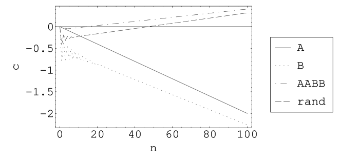
Figure 1: The expected capital $c(n)$ versus the number of steps $n$ for the Parrondo’s game with the sequence of strategies $A\cdots$ (solid line),$B\cdots$ (dotted line),$AABB\cdots$ (slashed-dotted line) and random choice (slashed line) of strategies. The biases of the coins are $p=\frac{1}{2}-\epsilon$, while for the coin $B$ is $p_{0}=\frac{1}{10}-\epsilon,p_{1}=\frac{3}{4}-\epsilon$, ($\epsilon=\frac{1}{100}$). The initial capital is equal to 0.

The time dependence of the expected capital is shown in Fig. 1.

Parrondo’s game may be thought of as a stochastic motion of a particle on the line [12]. For example (see Ref. [14]), any game driven by one coin which depends on the amount of capital modulo $L$ may be thought of as a stochastic motion on the line is governed by the master equation

$$P_{x}(n+1)=p_{x-1}P_{x-1}(n)+q_{x+1}P_{x+1}(n)\,,$$ (2)

where $P_{x}(n)$ is the probability that the capital amounts to $x$ after $n$ coin tosses, $p_{x}$ probability of the winning coin toss when capital is equal to $x$, and $q_{x}=1-p_{x}$ Eq. (2) is just the discretization of the Fokker-Planck equation

$$\frac{{\rm\partial}P(\xi,t)}{{\rm\partial}t}=-\frac{{\rm\partial}}{{\rm\partial}\xi}\left[F(\xi)P(\xi,t)\right]+\frac{1}{2}\frac{{\rm\partial}^{2}}{{\rm\partial}\xi^{2}}P(\xi,t)\,,$$ (3)

where $F(\xi)$ is the drift coefficient. The discrete version of $F(\xi)$ is $F_{x}=p_{x}-q_{x}$ and the Parrondo’s game is equivalent to the diffusion of a particle in the potential

$$V_{x}=-\frac{1}{2}\sum_{y=1}^{x}\ln\left(\frac{p_{x-1}}{1-p_{x}}\right)\,.$$ (4)

The mean position of the particle is equivalent to the expected capital. An application of the strategy is equivalent to turning on some potential, which will cause the particle to drift in a certain direction. The potential corresponding to the strategy $A$ is linear, while the capital (=position) dependence of the strategy $B$ is modelled by a sawtooth potential with a period equal to 3. By periodic switching of the potential on and off, the particle can drift in either direction. This is an example of a Brownian motor, when a thermal movement of the particle is directed by means of an external source with global (overall) zero effect.

3 Random choice of strategies with quantum walk

Quantum games which have properties of Parrondo’s game were proposed in Refs. [15, 16]. In Ref. [15] the authors considered a scheme which is essentially equivalent to our quantum walk scheme (see below), except that they do not use a qubit which “randomly” determines which strategy we use ($|d\rangle$ in our notation). Hence, they are constrained to deterministic strategies sequences. Moreover, the state of the quantum coin which determines whether we win or lose one unit of the capital is reset after each step. We decided to keep the state of the coin unchanged after each step, possibly enforcing quantum interference effects. Our model may lead to a higher rate of capital growth (see Fig. 4) depending on the initial state of the coin which affects the “random” choice of strategies.

In Ref. [16] the authors considered the quantization of a classical stochastic motion with a finite memory, which also leads to the Parrondo’s effect. This was attained by keeping the state of $n$ last “coin tosses” in a quantum register and using a sequence of unitary operators acting on one qubit of the register depending on the state of other qubits in the register. In what follows we will focus, on the “quantization” of a random sequence $AB\dots$. If the condition in Eq. (1) is satisfied, this game is winning.

There is no unique way how to quantize the Parrondo’s game. We should require that the amount of capital be encoded in the state of a quantum register with base states from $\mathcal{H}=\{|x\rangle:x\in\mathbb{Z}\}$. Classically, updating of the capital can be achieved by a random walk conditioned by the coins (strategies) $A,B$. The “quantization” of the random walk was performed in Ref. [17] as a controlled permutation on $\mathcal{H}$, with an additional register holding the result of the coin toss (unitary operation). The connection of this dynamics with a classical Markov process is shown in Ref. [18]: It may be thought of as a random walk in 1 dimension with an arbitrary bias to move in either direction, which contains an additional “interference” term between left and right steps in order to preserve the unitarity. For consistency, we can also use the quantum coin tosses for the simulation of random choice of strategies. Since the strategy $B$ requires dependence of the coin toss on the state of $|x\rangle$ modulo 3, we need an additional control qubit $|o\rangle$ which determines whether $x$ is divisible by 3 or not. This register can be reset after each application of the strategy, based on the information stored in other registers.

A quantum walk [17] is a unitary evolution (of a particle, for simplicity) similar to a discrete random walk. The state of the particle is a vector from the Hilbert space $\mathcal{H}$, which is spanned by the edges of some underlying oriented graph. We restrict ourselves to regular graphs.

Definition 3.1.

(Quantum walk in 1D) Let $\mathcal{H}_{C}=\mathrm{span}\{|c\rangle:c=0,1\}$ (the coin space), $\mathcal{H}_{X}=\mathrm{span}\{|x\rangle:x\in\mathbb{Z}\}$ (the position space) and $\mathcal{H}=\mathcal{H}_{C}\otimes\mathcal{H}_{X}$ be the Hilbert space of the quantum walk. Let $T_{0},T_{1}$ be operators on $\mathcal{H}_{X}$ such that $T_{0}|x\rangle=|x-1\rangle,T_{1}|x\rangle=|x+1\rangle$, $U\in SU(2)$ and $\pi_{j}=|j\rangle\langle j|,\;j=0,1$ be projection operators on $\mathcal{H}_{C}$. Then the evolution for one step of a quantum walk is given by a unitary operator

$$E=(\pi_{0}\otimes T_{0}+\pi_{1}\otimes T_{1})(U\otimes I)$$ (5)

The intuitive picture of the quantum walk in 1D is a particle endowed with an internal degree of freedom (chirality), which may take values 0 (left) and 1 (right), and whose state is rotated at each step by $U$. Then the particle takes a step to the left or to the right, depending on the chirality.

We introduce a new model of the quantum Parrondo’s game as follows: We have four registers $(\bm{C},\bm{D},\bm{X},\bm{O})$, states of which are described by vectors in Hilbert spaces $\mathcal{H}_{C},\mathcal{H}_{D},\mathcal{H}_{X},\mathcal{H}_{O}$, respectively. The register $\bm{X}$ stores the amount of capital; $\bm{D}$ is the coin register for the strategy used; $\bm{C}$ is the chirality register which determines the strategy we use; $\bm{O}$ is the auxiliary register. The quantum circuit which processes the data stored in these registers is shown in Fig. 2. The quantum Parrondo’s game is defined as

Definition 3.2.

(Quantum Parrondo’s game) We have $\mathcal{H}=\mathcal{H}_{C}\otimes\mathcal{H}_{D}\otimes\mathcal{H}_{X}\otimes\mathcal{H}_{O}$ such that:

1. The Hilbert spaces $\mathcal{H}_{j}=\mathrm{span}\{|k\rangle:k=0,1\}$ for $j\in\{C,D,O\}$. All operators on $\mathcal{H}_{j}$ will be henceforth written in the basis $(|0\rangle,|1\rangle)$, so that $|0\rangle=(1,0)^{T},|1\rangle=(0,1)^{T}$. The Hilbert space $\mathcal{H}_{X}=\mathrm{span}\{|x\rangle:x\in\mathbb{Z}\}$

2. $U$ is the unitary operator on $\mathcal{H}_{C}$:

   $$U=\frac{1}{\sqrt{2}}\left[\begin{array}[]{ll}1&{\rm i}\\ {\rm i}&1\end{array}\right].$$ (6)

3. The operator $X$ is the NOT gate:

   $$X=\left[\begin{array}[]{ll}0&1\\ 1&0\\ \end{array}\right].$$ (7)

4. The operator $\mathrm{c-}\!A$ is a controlled $SU(2)$ operator (rotation) on $\mathcal{H}_{C}\otimes\mathcal{H}_{D}$, the operators $\mathrm{c-}\!B_{0},\mathrm{c-}\!B_{1}$ are controlled $SU(2)$ operators on $\mathcal{H}_{D}\otimes\mathcal{H}_{C}\otimes\mathcal{H}_{O}$. In both cases, $\mathcal{H}_{D}$ is the target space. For any $SU(2)$ operator $G$ we use the parametrization

   $$G(\theta,\alpha,\beta)=\left[\begin{array}[]{ll}{\rm e}^{{\rm i}\alpha}\cos\frac{\theta}{2}&{\rm i}{\rm e}^{{\rm i}\beta}\sin\frac{\theta}{2}\\ {\rm i}{\rm e}^{-{\rm i}\beta}\sin\frac{\theta}{2}&{\rm e}^{-{\rm i}\alpha}\cos\frac{\theta}{2}\end{array}\right],$$ (8)

   with $\theta\in[0,\pi],\alpha,\beta\in[-\pi,\pi]$. We define

   $$\mathrm{c-}\!A=\pi_{0}\otimes A+\pi_{1}\otimes I\;;$$ (9)

   $$\mathrm{c-}\!B_{j}=\pi_{0}\otimes(B_{j}\otimes\pi_{0}+I\otimes\pi_{1})+\pi_{1}\otimes I\otimes I\;,$$ (10)

   for $j\in\{0,1\}$.

5. The gate $\mathrm{MOD}$ is the conditional operator:

   $$\mathrm{MOD}|x\rangle|o\rangle=\begin{cases}|x\rangle|o\rangle\quad 3\mid x\\ |x\rangle|o\oplus 1\rangle\quad\mathrm{otherwise.}\\ \end{cases}$$ (11)

6. The operator $S$ acting on $\mathcal{H}_{C}\otimes\mathcal{H}_{X}$ updates the $\bm{X}$ register (the capital by)

   $$S=\pi_{0}\otimes T_{0}+\pi_{1}\otimes T_{1},$$ (12)

   where $T_{0}|x\rangle=|x-1\rangle,T_{1}|x\rangle=|x+1\rangle$.

7. The gate $\mathrm{MOD_{inv}}$ acting on $\mathcal{H}_{C}\otimes\mathcal{H}_{X}\otimes\mathcal{H}_{O}$ ($\mathcal{H}_{O}$ is the target) is the conditional operator which resets the register $\bm{O}$. If the state of the $(\bm{C},\bm{X})$ register at the $n$-th step is $(c_{n},x_{n})$, we have $x_{n-1}\equiv x_{n}-(2c_{n}-1)\;(\mathrm{mod}\;3)$. At the $n$-th step, the operator $\mathrm{MOD}_{\mathrm{inv}}$ flips $|o\rangle$ if and only if $x_{n-1}\equiv 0\;(\mathrm{mod}\;3)$.

Figure 2: The quantum circuit for the quantum Parrondo’s game.

The logical circuit shown in Fig. 2 can be simplified to obtain the circuit presented in Fig. 3. In this circuit, the operator $W$ acting on $\mathcal{H}_{D}\otimes\mathcal{H}_{C}\otimes\mathcal{H}_{X}\otimes\mathcal{H}_{O}$ has the form

$$W=|0\rangle\langle 1|U\otimes\Big{[}B_{0}\otimes 1\otimes|1\rangle\langle 0|+B_{1}\otimes 1\otimes|0\rangle\langle 1|\Big{]}+|1\rangle\langle 0|U\otimes A\otimes 1\otimes X$$ (13)

and the operators $S,\mathrm{MOD}_{\mathrm{inv}}$ depend nontrivially only on $|c\rangle$.

Figure 3: A simplified version of the quantum circuit for the quantum Parrondo’s game.

We introduce a notation $\mathcal{H}_{W}\equiv\mathcal{H}_{D}\otimes\mathcal{H}_{C}$ and further we express the state of the whole system using the eigenvectors of the translation operator on $\mathcal{H}_{X}$:

$$|\phi_{k}^{j}\rangle=\sum_{\begin{subarray}{c}x\in\mathbb{Z};x\equiv j(\mathrm{mod}\;\,3)\end{subarray}}{\rm e}^{{\rm i}kx}|x\rangle,$$ (14)

for $j\in\{0,1,2\},k\in[-\pi,\pi]$. It is clear that $T_{0}|\phi_{k}^{j}\rangle=e^{ik}|\phi_{k}^{j\ominus 1}\rangle$ and $T_{1}|\phi_{k}^{j}\rangle=e^{-ik}|\phi_{k}^{j\oplus 1}\rangle$. We also set $|\phi_{k}\rangle=\sum_{j=0}^{2}|\phi_{k}^{j}\rangle$. The inverse transform is given by an expression

$$|x\rangle=\int_{-\pi}^{\pi}\frac{{\rm d}k}{2\pi}{\rm e}^{-{\rm i}kx}|\phi_{k}\rangle\;.$$ (15)

The action of $W\cdot\mathrm{MOD}$ on the state $|\chi\rangle|\phi_{k}^{j}\rangle|0\rangle$ gives

$$|\chi\rangle|\phi_{k}^{0}\rangle|0\rangle\mapsto \Big{(}\pi_{01}U\otimes B_{0}\otimes 1\otimes\pi_{10}+\pi_{10}U\otimes A\otimes 1\otimes X\Big{)}|\chi\rangle|\phi_{k}^{0}\rangle|0\rangle\;;$$ (16)

$$|\chi\rangle|\phi_{k}^{1,2}\rangle|0\rangle\mapsto \Big{(}\pi_{01}U\otimes B_{1}\otimes 1\otimes\pi_{01}+\pi_{10}U\otimes A\otimes 1\otimes X\Big{)}|\chi\rangle|\phi_{k}^{1,2}\rangle|1\rangle\;,$$ (17)

where $\pi_{ab}\equiv|a\rangle\langle b|$. Application of the operator $S$ and reseting the last register with $\mathrm{MOD}_{\mathrm{inv}}$ gives the evolution operator

$$E=\big{(}1_{D,C}\otimes 1_{X}\otimes\mathrm{MOD_{inv}}\big{)}\cdot S\cdot W\cdot\big{(}1_{D,C}\otimes 1_{X}\otimes\mathrm{MOD}\big{)}$$ (18)

whose action on $|\chi\rangle|\phi_{k}^{j}\rangle|0\rangle$ is

$$E|\chi\rangle|\phi_{k}\rangle|0\rangle=\Big{\{}(M_{10}+M_{11})|\chi\rangle|\phi_{k}^{0}\rangle+(M_{10}+M_{01})|\chi\rangle|\phi_{k}^{1}\rangle+(M_{11}+M_{00})|\chi\rangle|\phi_{k}^{2}\rangle\Big{\}}|0\rangle$$ (19)

with

$$M_{jd}={\rm e}^{s_{d}{\rm i}k}(\pi_{01}U\otimes\pi_{d}B_{j}+\pi_{10}U\otimes\pi_{d}A),$$ (20)

where $j,d\in\{0,1\},s_{d}=1-2d$. Multiple application of $E$ on the initial state gives

$$E^{n}|\chi\rangle|\phi_{k}\rangle|0\rangle=\Big{(}\mu_{0}^{(n)}|\chi\rangle|\phi_{k}^{1}\rangle+\mu_{1}^{(n)}|\chi\rangle|\phi_{k}^{1}\rangle+\mu_{2}^{(n)}|\chi\rangle|\phi_{k}^{2}\rangle\Big{)}|0\rangle\;.$$ (21)

The terms $M_{j}^{(n)}$ are related by the matrix-matrix equation

$$\left[\begin{array}[]{lll}\mu_{0}^{(n+1)}&\\ \mu_{1}^{(n+1)}&\\ \mu_{2}^{(n+1)}&\end{array}\right]=\left[\begin{array}[]{lll}0&M_{10}&M_{11}\\ M_{01}&0&M_{10}\\ M_{00}&M_{11}&0\end{array}\right]\cdot\left[\begin{array}[]{lll}\mu_{0}^{(n)}&\\ \mu_{1}^{(n)}&\\ \mu_{2}^{(n)}&\end{array}\right],$$ (22)

with $\mu_{j}^{(0)}=1$. The problem can be solved by computing the eigensystem of this $12\times 12$ matrix.

4 Numerical simulation of quantum Parrondo’s game

In this section we present results of numerical simulations of the quantum Parrondo’s game for different initial states. We assume a coin which is an analogue of the classical coins $A,B$; namely we consider $A=G(2(\frac{\pi}{2}-\epsilon),0,0),B_{0}=G(2(\frac{\pi}{10}-\epsilon),0,0),B_{1}=G(2(\frac{3}{4}-\epsilon),0,0),\epsilon=\frac{1}{100}$, We simulate the evolution for up to 1000 steps, counting the expected capital as

$$c(n)\equiv\sum_{x\in\mathbb{Z}}x\langle x|\rho_{X}(n)|x\rangle\;,$$ (23)

where

$$\rho_{X}(n)\equiv\mathrm{Tr}_{D,C,O}(E^{n})|\psi(0)\rangle\langle\psi(0)|(E^{\dagger})^{n}\,.$$ (24)

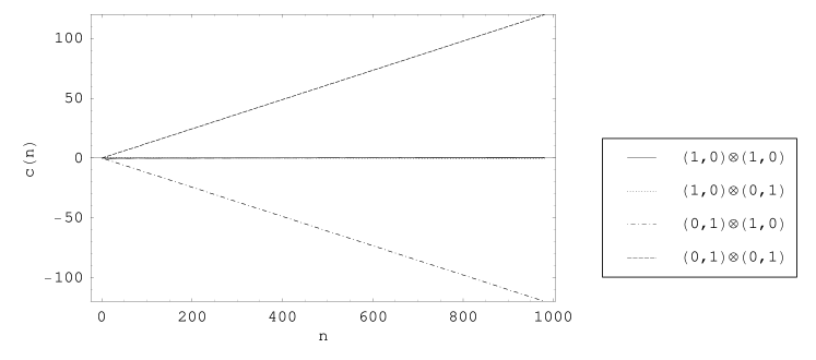
Figure 4: The expected capital $c(n)$ of the quantum Parrondo’s game for the zero initial capital and different initial states of the registers $(\bm{C},\bm{D})$.

For our purposes we observe four combinations of the basis states of $|d\rangle,|c\rangle$ (see Fig. 4). We see that the game may be winning, losing or fair, depending on the initial state of the register $|d\rangle|c\rangle$. The initial state of $|c\rangle$ determines whether the change in $c(n)$ is positive or negative (the two being symmetric), while the initial state of $|d\rangle$ determines the size of this change. The rate of losing/gaining the capital is much bigger than for the corresponding classical Parrondo’s game with random switching of the strategies (compare with Fig. 1).

The variance of the expected capital reads

$$v(n)\equiv\sum_{x\in\mathbb{Z}}x^{2}\langle x|\rho_{X}(n)|x\rangle\;.$$ (25)

It is easy to see that $v(n)$ does not depend on the initial state of the register $\bm{C}$, since the evolution is symmetric with respect to the exchange of directions. However, it does depend on the initial state of register $\bm{D}$, since this register determines the overall strategy. The numerical value of $v(n)$ is shown on Fig. 5.

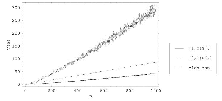
Figure 5: The variance $v(n)$ of the expected capital of the quantum Parrondo’s game for the zero initial capital and different initial states of register $\bm{D}$. The variance does not depend on the initial state of register $\bm{C}$. For comparison purposes we also simulate the variance for classical Parrondo’s game with random choice of strategies.

5 Random choice of strategies with CP-map

In Ref. [4] the author considered the difference between quantum strategies, and the mixed quantum strategies. In these mixed strategies one applies different unitary operators on the qubit with certain probabilities. It is probably a better analogue of a random sequence of classical strategies $A,B$ to consider quantum evolution, where the application of the operators $A,B_{0},B_{1}$ depends on a priori probabilities rather than on a state of the register $|d\rangle$. For our purposes, we discard the register $|d\rangle$ and the state of the game is described by a density operator

$$\rho=\sum_{x,y\in\mathbb{Z}}\rho_{xy}\otimes|x\rangle\langle y|\;.$$ (26)

We do not need to consider the state of the register $|o\rangle$, as any “garbage” information which is written into it is discarded by the operator $\mathrm{MOD}_{\mathrm{inv}}$. We need to reset the register $|o\rangle$ so that the projection $1\otimes 1\otimes\pi_{x}\otimes 1$ of the state vector $|\psi\rangle$ will effectively be from the subspace $\mathcal{H}_{D}\otimes\mathcal{H}_{C}$.

One step of the evolution of $\rho$ is described by the CP-map $\mathcal{E}$ such that (we omit the action of $\mathrm{MOD},\mathrm{MOD}_{\mathrm{inv}}$)

$$\mathcal{E}[\rho]=\sum_{j,k\in\{0,1\}}(\pi_{j}\otimes T_{j})\Big{[}\sum_{x,y\in\mathbb{Z}}\frac{1}{2}\big{(}A\rho_{xy}A^{\dagger}+B_{01}\rho_{xy}B_{01}^{\dagger}\big{)}\otimes|x\rangle\langle y|\Big{]}\big{(}\pi_{k}\otimes T_{k}\big{)}^{\dagger}\;.$$ (27)

Here $B_{01}$ depends on a state of the register $|o\rangle$ in the usual way. In this dynamics respective operators are applied with probabilities equal to $\frac{1}{2}$.

6 Numerical simulation of mixed Parrondo’s game

We have simulated the evolution of the mixed Parrondo’s game for different initial states of the register $|c\rangle$ and zero initial capital. The results (see Fig. 6) show that dynamics is different from both the random Parrondo’s game and the quantum Parrondo’s game in that the capital converges to a stationary value, which is either positive or negative, depending on the initial state of $|c\rangle$.

Figure 6: The capital of the mixed Parrondo’s game for zero initial capital and the initial state of the $\bm{C}$ register being $|0\rangle$ (1), $|1\rangle$ (2).

The expected capital resulting from the evolution given by Eq. (27) depends on the initial state in a symmetric way. To see this, let us consider the evolution

$$\mathcal{E}[(X\otimes 1)\rho(X^{\dagger}\otimes 1)]\;,$$ (28)

where $X$ is the swap operator on $\mathcal{H}_{C}$. It is obvious that $X$ commutes with $A$ and $B_{0},B_{1}$, and $(\pi_{L}\otimes T_{L}+\pi_{R}\otimes T_{R})(X\otimes 1)=(X\otimes 1)(\pi_{R}\otimes T_{L}+\pi_{L}\otimes T_{R})$. Hence, $n$ steps of the evolution with the swapped state give

$$\mathcal{E}^{n}[(X\otimes 1)\rho(X^{\dagger}\otimes 1)]=(X\otimes Y)\mathcal{E}^{n}[\rho](X\otimes Y)^{\dagger}\,,$$ (29)

where $Y|x\rangle=|-x\rangle$. The symmetry in the expected capital with respect to initial states $\pi_{L}\otimes\pi_{0}$ and $\pi_{R}\otimes\pi_{0}$ as seen in Fig. 6 immediately follows. The variance of the expected capital resulting from the mixed Parrondo’s game is shown in Fig. 7. Since the capital depends symmetrically on the initial state of $\bm{C}$, the variance is independent of it.

Figure 7: The variance of the expected capital of the mixed Parrondo’s game for zero initial capital and the initial state of the $\bm{C}$ register being either $|0\rangle$ or $|1\rangle$.

7 Conclusions: Connection between Parrondo’s games

The natural question arises: what is the connection between the three versions of Parrondo’s game we have considered in this paper? The quantum Parrondo’s game may be transformed into both the classical Parrondo’s game with quasi-random (memory dependent) strategies, and the mixed Parrondo’s game. To see this, let us consider that in the quantum Parrondo’s game we measure the register $\bm{D}$ at each step (just after the application of the operator $U$). If the initial state of $\bm{D}$ is either $|0\rangle$ or $|1\rangle$, the operator $U$ prepares equally weighed superposition of states $|0\rangle,|1\rangle$. Measurement of the register $\bm{D}$ gives a uniform probability distribution over $|0\rangle,|1\rangle$, hence the rest of the dynamics corresponds to random choice of strategies of $A,B$ and we obtain the mixed Parrondo’s game (compare Fig. 6 and Fig. 8).

Figure 8: The evolution of the capital which arises when we make a measurement of the register $\bm{C}$ immediately after we apply the operator $U$, averaged over 5000 samples. The initial state of $\bm{D}$ is $|0\rangle$ and the initial state of $\bm{C}$ is $|0\rangle$ (1),$|1\rangle$ (2).

Moreover, let us consider that we also measure the register $\bm{C}$ at each step (after the action of $A,B_{0},B_{1}$). Then the state of $|c\rangle$ collapses onto $|0\rangle,|1\rangle$ (with the biased probability) and the state of $|x\rangle$ is changed to the orthogonal state $|x\pm 1\rangle$. However, this evolution differs from the classical Parrondo’s game in that the bias of the coins depends on the outcome of the last measurement. To see this, let us consider that the initial state of $\bm{C}$ is $|0\rangle$ and in the first step we apply $A$. Then the new state of $\bm{C}$ is $[\sin\epsilon|0\rangle+{\rm i}\cos\epsilon|1\rangle]$ and the measurement on $|c\rangle$ gives $|0\rangle,|1\rangle$ with respective probabilities. If at the next step we happen to apply $A$ again, the new state of $\bm{C}$ will be either $[\sin\epsilon|0\rangle+{\rm i}\cos\epsilon|1\rangle]$ (if the last measurement gave $|0\rangle$) or $[\sin\epsilon|1\rangle+{\rm i}\cos\epsilon|0\rangle]$ otherwise. We see that the bias to measure $|0\rangle,|1\rangle$ changed (in classical terms, the new coin toss is more likely to win, if the last coin toss was losing, and vice versa).

In this paper we have shown how we can implement the Parrondo’s game with random switching of strategies using quantum formalism, and what is the difference between the “randomness” in the sense of quantum walks and the true randomness implemented via CP-maps. The first case leads to strictly positive or negative gain in the capital, or even to zero outcome, depending on the initial state of the coin registers. The second case may also lead to the positive or negative gain; however the capital converges to a fixed value. The measurement of a selected register may reduce the quantum Parrondo’s game to the mixed Parrondo’s game, and hence suppress the winning ratio of the game.

Finally, we note that there exist other versions of the quantum Parrondo’s game. Specifically, in Ref. [19] the authors discussed how the paradox arises when coin tosses depend on the states of the coins at the previous steps. Cooperative Parrondo’s game are also of interest. The problem of coins with memories and other modifications of Parrondo’s game as well as physical realization of the game via quantum walks will be presented elsewhere.

Acknowledgments: We thank Mark Hillery and Jason Twamley for helpful discussions. This research was supported in part by the European Union projects QAP, CONQUEST, by the INTAS project 04-77-7289, by the Slovak Academy of Sciences via the project CE-PI/2/2005, and by the project APVT-99-012304. The project was also partially funded by Polish Ministry of Science and Higher Education grant number N519 012 31/1957.

References

- [1] J. von Neumann and O. Morgenstern, Theory of games and economic behavior (Princeton University Press, Princeton, 1953).
- [2] J. Eisert, M. Wilkens M, and M. Lewenstein, Phys. Rev. Lett. 83, 3077 (1999).
- [3] J. Nash, The Annals of Mathematics 54, 286 (1951).
- [4] D. A. Meyer, Phys. Rev. Lett. 82, 1052 (1999).
- [5] B. C. Sanders, S. D. Bartlett, B. Tregenna, and P. L. Knight, Phys. Rev. A 67, 042305 (2003).
- [6] P. L. Knight, E. Roldan, and J. E. Sipe, Phys. Rev. A 68, 020301 (2003).
- [7] P. L. Knight, E. Roldan, and J. E. Sipe, Optics Communications 227, 147 (2003).
- [8] P. L. Knight, E. Roldan, and J. E. Sipe, J. Mod. Opt. 51, 1761 (2004).
- [9] I. Carneiro, M. Loo, X. B. Xu, M. Girerd, V. Kendon, and P. L. Knight, New Journal of Physics 8, 156 (2005).
- [10] G. P. Harmer and D. Abbott, Nature 402, 864 (1999).
- [11] J. M. R. Parrondo, G. P. Harmer, and D. Abbott, Phys. Rev. Lett. 85, 5226 (2000).
- [12] J. Parrondo and L. Dinís, Contemporary Physics 45, 147 (2004).
- [13] D. A. Meyer and H. Blumer, Journal of Statistical Physics 107, 225 (2002).
- [14] R. Toral, P. Amengual, and S. Mangioni, Physica A 327, 105 (2003).
- [15] J. A. Miszczak and P. Gawron, Fluctuation and Noise Letters 5, (2005).
- [16] A. P. Flitney, J. Ng, and D. Abbott, Physica A 314, 35 (2002).
- [17] Y. Aharonov, L. Davidovich, and N. Zagury, Phys. Rev. A 48, 1687 (1993).
- [18] A. Romanelli, A. C. Sicardi Schifino, R. Siri, G. Abal, A. Auyuanet, and R. Donangelo, Physica A 338, 395 (2004).
- [19] A. P. Flitney, D. Abbott, and N. F. Johnson, Quantum random walks with history dependence. Available online at: http://arxiv.org/abs/quant-ph/0311009v1.