Multiple scalar particle decay
and perturbation generation

Abstract:

We study the evolution of the universe which contains a multiple number of non-relativistic scalar fields decaying into both radiation and pressureless matter. We present a powerful analytic formalism to calculate the matter and radiation curvature perturbations, and find that our analytic estimates agree with full numerical results within an error of less than one percent. Also we discuss the isocurvature perturbation between matter and radiation components, which may be detected by near future cosmological observations, and point out that it crucially depends on the branching ratio of the decay rate of the scalar fields and that it is hard to make any model independent predictions.

1 Introduction

Nowadays it is widely accepted that the primordial density perturbations are the origin of the temperature anisotropy in the cosmic microwave background (CMB) and large scale structure in the present observable universe. Various cosmological observations indicate that these perturbations are adiabatic and Gaussian, with an almost scale invariant spectrum [1]. Interestingly, these observational facts are consistent with an earlier inflationary era [2]: during inflation, quantum fluctuations of a slowly rolling scalar field which dominates the energy density, the inflaton, are stretched and become classical perturbations due to the quasi exponential expansion of the universe. A particularly convenient quantity to study these perturbations is the curvature perturbation $\zeta$ on uniform density hypersurfaces, developed in [3], or $\mathcal{R}_{c}$ on comoving hypersurfaces which is equivalent to $\zeta$ on large scales. For single field inflation cases $\zeta$ is known to be conserved on large scales since perturbations are purely adiabatic, and one can obtain the power spectrum of these perturbations with good enough accuracy [4]. Note that, in multi-field inflationary models, in contrast, there exists in general a non-adiabatic pressure perturbation and this makes $\zeta$ no more conserved on large scales [6].

In conventional inflationary models, the inflaton field is assumed to play two roles at the same time: it dominates the energy density during inflation and makes the universe expand enough to solve many cosmological problems such as homogeneity, isotropy and flatness of the observable universe. Also, its vacuum fluctuations are relevant for the curvature perturbation $\zeta$ and thus responsible for the primordial density perturbations. Generally, the latter requirement introduce extra fine tuning into the model: for example, in the simplest chaotic inflation model with $V(\phi)=m^{2}\phi^{2}/2$, the inflaton mass $m$ can be as large as $\mathcal{O}({m_{\mathrm{Pl}}})$, where ${m_{\mathrm{Pl}}}=(8\pi G)^{-1/2}\approx 2.4\times 10^{18}\,\textrm{GeV}$ is the reduced Planck mass, when we do not mind perturbations and try to solve other problems. However, to match the observed amplitude of density perturbations on large scales, we need $m\sim\mathcal{O}\left(10^{-5}\right){m_{\mathrm{Pl}}}$, i.e. we need a relative fine tuning of one part over $10^{5}$ [7]. However, during inflation, any scalar fields with their masses being smaller than the Hubble scale acquire almost scale invariant fluctuations. Such fields, depending on the post-inflationary evolution of the universe, may later generate primordial density perturbations by transferring their almost scale invariant isocurvature perturbations to the curvature perturbation.

If this is the case, i.e. in the so-called curvaton scenario [9], such a field, dubbed the “curvaton”, should satisfy several requirements: firstly, its effective mass must be light, i.e. less than the Hubble parameter during inflation, to produce an almost flat spectrum of fluctuations and to remain sub-dominant during inflation. It should also couple very weakly to other fields so that its potential in the early universe is not modified appreciably. It is also demanded that it keeps some level of non-zero value [10] and has not yet relaxed to its vacuum expectation value. This is necessary to generate the appropriate amplitude of perturbations. These conditions are basically what the conventional inflaton field should satisfy, which is assumed to be responsible for the primordial density perturbations, as well as the enough expansion of the universe. Thus, the curvaton scenario may find its natural accommodation in the context of multi-field inflation [11]: for example, in a recently proposed scenario [12] where a number of string axion fields drive inflation, it is known [13] that there are a number of fields which have not yet relaxed to their minima of the effective potential, with their mass being very small relative to the Hubble parameter during inflation due to the assisted inflation mechanism [14].

Therefore, it is natural to consider the case where multiple curvaton fields are responsible for the generation of the curvature perturbation after inflation. The fluctuations of these curvaton fields are non-adiabatic in nature and thus, as mentioned above, the curvature perturbation $\zeta$ does not remain constant but evolves according to the energy transfer between different components which constitute the universe. In this paper we study this general curvaton model. This paper is outlined as follows. In Sec. 2, we introduce the coupled equations which determine the evolution of the universe. In Sec. 3 we solve these equations analytically using the so-called sudden decay approximation, using a novel and model independent method. In Sec. 4 we apply our results of the previous sections to several examples and compare the analytic estimates with numerical calculations. Finally in Sec. 5 we summarise and present our conclusions.

2 Background equations and perturbations

In this section we will summarise the evolution of the background quantities in a flat universe and show the evolution equations of the curvature perturbations of the components in the system of multiple curvatons decaying into radiation and matter. We assume that the universe is initially dominated by radiation due to the decay of the inflaton field(s) after inflation.

We assume that the curvatons ($\sigma_{i}$) decay into both radiation ($\gamma$) and non-relativistic matter ($m$) with constant decay rates ${\Gamma_{\gamma}^{(i)}}$ and ${\Gamma_{m}^{(i)}}$ respectively, which are fixed by underlying physics. The energy transfer equations between components are given by

$$Q_{i} =-({\Gamma_{\gamma}^{(i)}}+{\Gamma_{m}^{(i)}})\rho_{i}\equiv-{\Gamma^{(i)}}\rho_{i}\,,$$ (1)

$$Q_{\gamma} =\sum_{i}{\Gamma_{\gamma}^{(i)}}\rho_{i}\equiv\sum_{i}Q_{\gamma i}\,,$$ (2)

$$Q_{m} =\sum_{i}{\Gamma_{m}^{(i)}}\rho_{i}\equiv\sum_{i}Q_{mi}\,,$$ (3)

where we have introduced the total decay width of $\sigma_{i}$, ${\Gamma^{(i)}}\equiv{\Gamma_{\gamma}^{(i)}}+{\Gamma_{m}^{(i)}}$, and the energy transfer to radiation (matter) by the decay of $\sigma_{i}$, $Q_{\gamma i}$ ($Q_{mi}$), respectively. Note that they obey the constraint of energy conservation

$$\begin{split}\sum_{i}Q_{i}+Q_{\gamma}+Q_{m}=0\,.\end{split}$$ (4)

Thus from the general continuity equation of each component including energy transfer [16],

$$\dot{\rho}_{\alpha}=-3H(\rho_{\alpha}+p_{\alpha})+Q_{\alpha}\,,$$ (5)

we find that for each component

$$\dot{\rho}_{i} =-(3H+\Gamma^{(i)})\rho_{i}\,,$$ (6)

$$\dot{\rho}_{\gamma} =-4H\rho_{\gamma}+\sum_{i}\Gamma_{\gamma}^{(i)}\rho_{i}\,,$$ (7)

$$\dot{\rho}_{m} =-3H\rho_{m}+\sum_{i}\Gamma_{m}^{(i)}\rho_{i}\,.$$ (8)

Note that we can obtain the continuity equation of the total energy density by summing over that of each component,

$$\dot{\rho} =-3H(\rho+p)$$

$$=-H\left(4\rho_{\gamma}+3\rho_{m}+3\sum_{i}\rho_{i}\right)\,,$$ (9)

where the total density $\rho$ and pressure $p$ are given by

$$\rho =\rho_{\gamma}+\rho_{m}+\sum_{i}\rho_{i}\,,$$ (10)

$$p =p_{\gamma}+p_{m}+\sum_{i}p_{i}\,,$$ (11)

respectively. In the above we take $p_{\gamma}=\rho_{\gamma}/3$ and $p_{m}=p_{i}=0$, i.e. the equation of state of the curvaton fields are effectively equivalent to that of pressureless matter.

By adopting the density parameters $\Omega_{\gamma}$, $\Omega_{m}$ and $\Omega_{i}$, we can rewrite Eqs. (6), (7) and (8) in more convenient dimensionless forms for numerical calculation. From the Friedmann equation

$$H^{2}=\frac{1}{3m_{\mathrm{Pl}}^{2}}\rho\,,$$ (12)

the density parameters satisfy the relation

$$\Omega_{\gamma}+\Omega_{m}+\sum_{i}\Omega_{i}=1\,.$$ (13)

Then, Eqs. (6), (7) and (8) can be written as

$$\Omega_{i}^{\prime} =\Omega_{i}\left(\Omega_{\gamma}-H^{-1}{\Gamma^{(i)}}\right)\,,$$ (14)

$$\Omega_{\gamma}^{\prime} =H^{-1}\sum_{i}\Omega_{i}{\Gamma_{\gamma}^{(i)}}-\Omega_{\gamma}(1-\Omega_{\gamma})\,,$$ (15)

$$\Omega_{m}^{\prime} =H^{-1}\sum_{i}\Omega_{i}{\Gamma_{m}^{(i)}}+\Omega_{\gamma}\Omega_{m}\,,$$ (16)

and Eq. (12) as

$$H^{\prime}=-\frac{3+\Omega_{\gamma}}{2}H\,,$$ (17)

where a prime denotes a derivative with respect to the number of $e$-folds,

$$N\equiv\int Hdt\,.$$ (18)

The total curvature perturbation on uniform curvature hypersurfaces is given by

$$\zeta=-H\frac{\delta\rho}{\dot{\rho}}\,,$$ (19)

which can be written as a weighted sum of the curvature perturbation of the component $\alpha$ on the corresponding uniform density hypersurfaces $\zeta_{\alpha}$ [6],

$$\zeta=\sum_{\alpha}\frac{\dot{\rho}_{\alpha}}{\dot{\rho}}\zeta_{\alpha}\,,$$ (20)

where

$$\zeta_{\alpha}=-H\frac{\delta\rho_{\alpha}}{\dot{\rho}_{\alpha}}\,.$$ (21)

The difference between any two components gives an isocurvature perturbation [17]

$$\mathcal{S}_{\alpha\beta}=3(\zeta_{\alpha}-\zeta_{\beta})\,.$$ (22)

The total curvature perturbation on large scales evolves as [6]

$$\dot{\zeta}=-\frac{H}{\rho+p}\delta p_{\mathrm{nad}}\,,$$ (23)

where the non-adiabatic pressure perturbation is given by

$$\delta p_{\mathrm{nad}}\equiv\delta p-\frac{\dot{p}}{\dot{\rho}}\delta\rho\,.$$ (24)

Therefore, as mentioned before, $\zeta$ remains constant on large scales when the perturbations are purely adiabatic. From Eqs. (21) and (23), and using the perturbed continuity equations of each component [17, 18], we can find that the curvature perturbations of the components evolve on large scales as

$$\zeta_{i}^{\prime} =\frac{H^{-1}{\Gamma^{(i)}}(3+\Omega_{\gamma})}{2\left(3+H^{-1}{\Gamma^{(i)}}\right)}\left(\zeta-\zeta_{i}\right)\,,$$ (25)

$$\zeta_{\gamma}^{\prime} =\left(4\Omega_{\gamma}-H^{-1}\sum_{i}{\Gamma_{\gamma}^{(i)}}\Omega_{i}\right)^{-1}\left[\sum_{j}\Omega_{j}(3+H^{-1}{\Gamma^{(i)}})H^{-1}{\Gamma_{\gamma}^{(i)}}\left(\zeta_{i}-\zeta_{\gamma}\right)\right.$$

$$\hskip 156.49014pt\left.-\frac{H^{-1}\sum_{k}\Gamma_{\gamma}^{(k)}\Omega_{k}}{2}(3+\Omega_{\gamma})\left(\zeta-\zeta_{\gamma}\right)\right]\,,$$ (26)

$$\zeta^{\prime} =\frac{4\Omega_{\gamma}-H^{-1}\sum_{i}{\Gamma_{\gamma}^{(i)}}\Omega_{i}}{3+\Omega_{\gamma}}\left(\zeta-\zeta_{\gamma}\right)\,.$$ (27)

Here we do not solve the evolution of $\zeta_{m}$ directly, though it is straightforward to write the evolution equation of $\zeta_{m}$: rather, from Eq. (20), $\zeta_{m}$ is calculated as

$$\zeta_{m}=\frac{\dot{\rho}\zeta-\dot{\rho}_{\gamma}\zeta_{\gamma}-\sum_{i}\dot{\rho}_{i}\zeta_{i}}{\dot{\rho}_{m}}\,.$$ (28)

The reason is the existence of singularity in $\zeta_{m}$, because there exists some moment $\dot{\rho}_{m}=0$ when the dilution of matter due to the expansion of the universe is balanced with the creation of matter due to the curvaton decay [17, 18].

We may solve Eqs. (14)–(17) and (25)–(27) numerically, which would be the simplest way to study the evolution of the curvature perturbation. However, we can obtain further insights by implementing analytic analysis. In the following section we will find the final curvature perturbations under the so-called sudden decay approximation [19].

3 Analytic approximation

In this section, we study the curvature perturbations under the assumption that there is no interaction between components until the curvaton fields decay and that the decay of each curvaton is instantaneous. Under this “sudden decay approximation”, we can derive analytic estimates for the curvature perturbations associated with matter and radiation after all the curvaton fields decay, as we will see in this section. Note that from Eqs. (1), (2) and (3), after all the curvatons decay, there is no energy transfer between matter and radiation and hence $\zeta_{m}$ and $\zeta_{\gamma}$ are constant, though $\zeta$ will still evolve on large scales. In this sense, we will call these $\zeta_{m}$ and $\zeta_{\gamma}$ after the decay of the curvatons as “final” curvature perturbations, and denote by the superscript (out).

For our purpose in this section, we decompose the radiation and matter density according to the source of generation,

$$\begin{split}\rho_{\gamma}&={\rho_{\gamma 0}}+\sum_{i}{\rho_{\gamma i}},\\ \rho_{m}&=\rho_{m0}+\sum_{i}\rho_{mi},\end{split}$$ (29)

where ${\rho_{\gamma 0}}$ ($\rho_{m0}$) is the energy density of radiation (matter) which is due to the decay of the inflaton field(s) and independent of the curvaton decay, and ${\rho_{\gamma i}}$ ($\rho_{mi}$) is the radiation (matter) density generated from the decay of $\sigma_{i}$ [20]. Then, Eq. (10) can be written as

$$\rho ={\rho_{\gamma 0}}+\rho_{m0}+\sum_{i}\left({\rho_{\gamma i}}+\frac{{\Gamma_{\gamma}^{(i)}}}{{\Gamma^{(i)}}}\rho_{i}\right)+\sum_{i}\left(\rho_{mi}+\frac{{\Gamma_{m}^{(i)}}}{{\Gamma^{(i)}}}\rho_{i}\right)$$

$$\equiv{\rho_{\gamma 0}}+\rho_{m0}+\sum_{i}\widetilde{\rho}_{\gamma i}+\sum_{i}\widetilde{\rho}_{mi}\,,$$ (30)

where we have introduced two composite densities $\widetilde{\rho}_{\gamma i}$ and $\widetilde{\rho}_{mi}$ which will play the central role in the discussions below.

3.1 Matter curvature perturbation

From Eqs. (1), (3) and (3), we can see that for the composite density $\widetilde{\rho}_{mi}$,

$$\widetilde{Q}_{mi}=Q_{mi}+\frac{{\Gamma_{m}^{(i)}}}{{\Gamma^{(i)}}}Q_{i}=0\,,$$ (31)

i.e. the energy transfer is zero. Moreover, since the corresponding equation of state is that of pressureless matter, we can write

$$\dot{\widetilde{\rho}}_{mi}=-3H\widetilde{\rho}_{mi}\,,$$ (32)

and therefore the associated curvature perturbation [18],

$$\widetilde{\zeta}_{mi}=-H\frac{\delta\widetilde{\rho}_{mi}}{\dot{\widetilde{\rho}}_{mi}}=\frac{\delta\widetilde{\rho}_{mi}}{3\widetilde{\rho}_{mi}}\,,$$ (33)

is conserved on large scales. Well before the curvaton $\sigma_{i}$ decays $\rho_{mi}=\delta\rho_{mi}=0$ so $\widetilde{\zeta}_{mi}=\zeta_{i}^{\mathrm{(in)}}$, meanwhile after $\sigma_{i}$ decays $\rho_{i}$ is negligible and thus $\widetilde{\zeta}_{mi}=\zeta_{mi}^{\mathrm{(out)}}$. Therefore we have

$$\zeta_{mi}^{\mathrm{(out)}}=\zeta_{i}^{\mathrm{(in)}}\,.$$ (34)

Thus, from Eqs. (21), (29) and (34), we find that the final matter curvature perturbation after all the curvatons decay is given by

$$\zeta_{m}^{\mathrm{(out)}} =\left(\rho_{m0}^{\mathrm{(in)}}\zeta_{m0}^{\mathrm{(in)}}+\sum_{i}\frac{{\Gamma_{m}^{(i)}}}{{\Gamma^{(i)}}}\rho_{i}^{\mathrm{(in)}}\zeta_{i}^{\mathrm{(in)}}\right)\left[\rho_{m0}^{\mathrm{(in)}}+\sum_{j}\frac{\Gamma_{m}^{(j)}}{\Gamma^{(j)}}\rho_{j}^{\mathrm{(in)}}\right]^{-1}$$

$$\equiv\sum_{i=0}^{n}s_{i}\zeta_{i}^{\mathrm{(in)}}\,,$$ (35)

where $\zeta_{0}^{\mathrm{(in)}}\equiv\zeta_{m0}^{\mathrm{(in)}}$. The transfer coefficient $s_{i}$ we have introduced above is given by

$$s_{0} =\Omega_{m0}^{\mathrm{(in)}}\left[\Omega_{m0}^{\mathrm{(in)}}+\sum_{j}\frac{\Gamma_{m}^{(j)}}{\Gamma^{(j)}}\Omega_{j}^{\mathrm{(in)}}\right]^{-1}\,,$$

$$s_{i} =\frac{{\Gamma_{m}^{(i)}}}{{\Gamma^{(i)}}}\Omega_{i}^{\mathrm{(in)}}\left[\Omega_{m0}^{\mathrm{(in)}}+\sum_{j}\frac{\Gamma_{m}^{(j)}}{\Gamma^{(j)}}\Omega_{j}^{\mathrm{(in)}}\right]^{-1}\,.\hskip 14.22636pt(i=1,2,\cdots,n)$$ (36)

So we can see that the final matter curvature perturbation is completely determined by the decay rate and the initial energy density $\rho_{i}^{\mathrm{(in)}}$, or equivalently, initial density parameter $\Omega_{i}^{\mathrm{(in)}}$ of each curvaton field and that of pre-existing matter as shown above.

3.2 Radiation curvature perturbation

In the previous section, we could use the conservation of the curvature perturbation of each composite density $\widetilde{\rho}_{mi}$ to find out the final matter curvature perturbation. This is possible since every $\widetilde{\rho}_{mi}$ has no energy transfer and in addition unique equation of state. One may hope that similar argument is applied to the other composite density we have introduced in Eq. (3), $\widetilde{\rho}_{\gamma i}$, but this is not the case. Nevertheless, $\widetilde{\rho}_{\gamma i}$ turns out to be an useful quantity to calculate the final radiation curvature perturbation as we will see shortly. In this section, we assume that the decay rates of the curvaton fields are different so that they do not decay at the same time: rather, they decay successively due to different decay rates. Without loss of generality we put the order of curvatons by the decay rate of each curvaton to satisfy ${\Gamma^{(i)}}>\Gamma^{(i+1)}$.

First we consider a limited time interval around the decay of the curvaton field $\sigma_{1}$, which is assumed to have the largest decay rate. We write a combined density of radiation and the curvaton field

$$\rho_{\gamma}^{(1)} \equiv{\rho_{\gamma 0}}+\widetilde{\rho}_{\gamma 1}$$

$$={\rho_{\gamma 0}}+\rho_{\gamma 1}+\frac{\Gamma_{\gamma}^{(1)}}{\Gamma^{(1)}}\rho_{1}\,.$$ (37)

Note that although the energy transfer of $\rho_{\gamma}^{(1)}$ is zero, its equation of state is not unique and thus the corresponding curvature perturbation $\zeta_{\gamma}^{(1)}$ evolves on large scales. Therefore, as mentioned above, unlike $\widetilde{\rho}_{mi}$ we cannot simply connect the initial curvature perturbations in the curvaton fields to the final one in radiation, but rather we have to get through the moments of decay. Now we assume that until $\sigma_{1}$ decays instantaneously there is no energy transfer between the curvaton and radiation. Then, $\rho_{\gamma}^{(1)}$ before and after $\sigma_{1}$ decays, which we write respectively

$$\rho_{\gamma}^{(1)}|_{\mathrm{before}} ={\rho_{\gamma 0}}^{<1}+\frac{\Gamma_{\gamma}^{(1)}}{\Gamma^{(1)}}\rho_{1}^{<1}\,,$$ (38)

$$\rho_{\gamma}^{(1)}|_{\mathrm{after}} ={\rho_{\gamma 0}}^{>1}+\rho_{\gamma 1}^{>1}\,,$$ (39)

where the superscript $<1$ ($>1$) means that it is evaluated before (after) $\sigma_{1}$ decays, and these densities have the same value at the moment of decay. Since $\rho_{\gamma 1}$ is generated only after $\sigma_{1}$ decays, the value of $\rho_{\gamma 1}$ at the moment of decay corresponds to its initial value and thus

$$\rho_{\gamma 1}^{\mathrm{(dec)}}=\frac{\Gamma_{\gamma}^{(1)}}{\Gamma^{(1)}}\rho_{1}^{\mathrm{(dec)}}\,.$$ (40)

Using the fact that both ${\rho_{\gamma 0}}$ and $\rho_{\gamma 1}$ scale as $a^{-4}$, we can write the ratio $\rho_{\gamma 1}/{\rho_{\gamma 0}}$ at late times, which is constant after $\sigma_{1}$ decays, as

$$\frac{\rho_{\gamma 1}}{{\rho_{\gamma 0}}}=\frac{\rho_{\gamma 1}^{\mathrm{(dec)}}(a^{\mathrm{(dec)}}/a)^{4}}{{\rho_{\gamma 0}}^{\mathrm{(dec)}}(a^{\mathrm{(dec)}}/a)^{4}}=\frac{\Gamma_{\gamma}^{(1)}}{\Gamma^{(1)}}\frac{\rho_{1}^{\mathrm{(dec)}}}{{\rho_{\gamma 0}}^{\mathrm{(dec)}}}\,.$$ (41)

The individual curvature perturbations $\zeta_{\gamma 0}$ and $\zeta_{1}$ remain constant on large scales before $\sigma_{1}$ decays. Then, the combined curvature perturbation $\zeta_{\gamma}^{(1)}$ corresponding to $\rho_{\gamma}^{(1)}$ is written as

$$\zeta_{\gamma}^{(1)}\approx(1-f_{1})\zeta_{\gamma 0}+f_{1}\zeta_{1}\,,$$ (42)

where

$$f_{1}=\frac{3\frac{\Gamma_{\gamma}^{(1)}}{\Gamma^{(1)}}\rho_{1}}{4{\rho_{\gamma 0}}+3\frac{\Gamma_{\gamma}^{(1)}}{\Gamma^{(1)}}\rho_{1}}\,.$$ (43)

Here $f_{1}$, the weight of $\zeta_{1}$, solely describes the evolution of $\zeta_{\gamma}^{(1)}$ on large scales. After the curvaton $\sigma_{1}$ decays, the energy density $\rho_{\gamma}^{(1)}$ is identical to $\rho_{\gamma}$ at that time and has a unique equation of state. Hence after the decay of $\sigma_{1}$, $\zeta_{\gamma}^{(1)}$ becomes constant on large scales until the curvaton with the next largest decay width begins to decay, i.e. [17]

$$\zeta_{\gamma}^{>1}=\zeta_{\gamma}^{(1)}|_{\mathrm{dec}}\approx\left(1-f_{1}^{\mathrm{(dec)}}\right)\zeta_{\gamma 0}^{\mathrm{(in)}}+f_{1}^{\mathrm{(dec)}}\zeta_{1}^{\mathrm{(in)}}\,,$$ (44)

where, using Eq. (41), $f_{1}^{\mathrm{(dec)}}$ is given by

$$f_{1}^{\mathrm{(dec)}}=\frac{3\rho_{\gamma 1}/{\rho_{\gamma 0}}}{4+3\rho_{\gamma 1}/{\rho_{\gamma 0}}}\,.$$ (45)

We can take the same step for the successive curvaton decays: e.g. for $\sigma_{2}$ which has the next largest decay width, we just replace

$$\rho_{\gamma}^{(1)}|_{\mathrm{after}} \Rightarrow\rho_{\gamma 0\mathrm{(new)}}\,,$$

$$\zeta_{\gamma}^{>1} \Rightarrow\zeta_{\gamma 0\mathrm{(new)}}\,,$$ (46)

and so on. In general after $i$-th curvaton $\sigma_{i}$ decays, the curvature perturbation in the radiation component is constant until the decay of $(i+1)$-th curvaton, and is written as

$$\zeta_{\gamma}^{>i}\approx\left(1-f_{i}^{\mathrm{(dec)}}\right)\zeta_{\gamma}^{>i-1}+f_{i}^{\mathrm{(dec)}}\zeta_{i}^{\mathrm{(in)}}\,,$$ (47)

where

$$f_{i}^{\mathrm{(dec)}}=\frac{3{\rho_{\gamma i}}/{\rho_{\gamma 0}}}{4\sum_{k=0}^{i-1}\rho_{\gamma k}/{\rho_{\gamma 0}}+3{\rho_{\gamma i}}/{\rho_{\gamma 0}}}\,.$$ (48)

Therefore, after all the $n$ curvatons decay, we find the final curvature perturbations in radiation as

$$\zeta_{\gamma}^{\mathrm{(out)}} \approx\left(1-f_{n}^{\mathrm{(dec)}}\right)\zeta_{\gamma}^{>n-1}+f_{n}^{\mathrm{(dec)}}\zeta_{n}^{\mathrm{(in)}}$$

$$=\left(1-f_{n}^{\mathrm{(dec)}}\right)\left(1-f_{n-1}^{\mathrm{(dec)}}\right)\zeta_{\gamma}^{>n-2}+\left(1-f_{n}^{\mathrm{(dec)}}\right)f_{n-1}^{\mathrm{(dec)}}\zeta_{n-1}^{\mathrm{(in)}}+f_{n}^{\mathrm{(dec)}}\zeta_{n}^{\mathrm{(in)}}$$

$$=\cdots$$

$$\equiv\sum_{i=0}^{n}r_{i}\zeta_{i}^{\mathrm{(in)}}\,,$$ (49)

where $\zeta_{0}^{\mathrm{(in)}}\equiv\zeta_{\gamma 0}^{\mathrm{(in)}}$ and $f_{0}^{\mathrm{(dec)}}=1$. The transfer coefficient $r_{i}$ is given by

$$r_{i} =\prod_{k=i+1}^{n}\left(1-f_{k}^{\mathrm{(dec)}}\right)f_{i}^{\mathrm{(dec)}}=\left(1-\sum_{k=i+1}^{n}r_{k}\right)f_{i}^{\mathrm{(dec)}}\,,\hskip 14.22636pt(i=0,1,\cdots,n-1)$$

$$r_{n} =f_{n}^{\mathrm{(dec)}}\,,$$ (50)

and is completely determined once we find the ratio ${\rho_{\gamma i}}/{\rho_{\gamma 0}}$.

3.3 Ratio of radiation after curvaton decay

We found in the previous section that the final radiation curvature perturbation depends on the ratio of the radiation generated from curvaton decay with respect to the original radiation component. In this section, we present a general and simple way to calculate this ratio analytically.

From Eqs. (6), (7) and (8), we can write the continuity equations of the components used in Eq. (3) as

$$\dot{\rho}_{\gamma 0} =-4H{\rho_{\gamma 0}}\,,$$ (51)

$$\dot{\rho}_{m0} =-3H\rho_{m0}\,,$$ (52)

$$\dot{\widetilde{\rho}}_{\gamma i} =-4H{\rho_{\gamma i}}-3H\frac{{\Gamma_{\gamma}^{(i)}}}{{\Gamma^{(i)}}}\rho_{i}\,,$$ (53)

$$\dot{\widetilde{\rho}}_{mi} =-3H\rho_{mi}-3H\frac{{\Gamma_{m}^{(i)}}}{{\Gamma^{(i)}}}\rho_{i}\,.$$ (54)

We can solve these equation analytically and the solutions are given by

$${\rho_{\gamma 0}} =\rho_{\gamma 0}^{\mathrm{(in)}}\left(\frac{a^{\mathrm{(in)}}}{a}\right)^{4}\,,$$ (55)

$$\rho_{m0} =\rho_{m0}^{\mathrm{(in)}}\left(\frac{a^{\mathrm{(in)}}}{a}\right)^{3}\,,$$ (56)

$$\rho_{i} =\rho_{i}^{\mathrm{(in)}}\left(\frac{a^{\mathrm{(in)}}}{a}\right)^{3}\exp\left[-{\Gamma^{(i)}}(t-t_{0})\right]\,,$$ (57)

$${\rho_{\gamma i}} ={\Gamma_{\gamma}^{(i)}}\rho_{i}^{\mathrm{(in)}}\left(\frac{a^{\mathrm{(in)}}}{a}\right)^{4}\int_{t_{0}}^{t}\frac{a}{a^{\mathrm{(in)}}}\exp\left[-{\Gamma^{(i)}}t^{\prime}\right]dt^{\prime}\,,$$ (58)

$$\rho_{mi} =\frac{{\Gamma_{m}^{(i)}}}{{\Gamma^{(i)}}}\rho_{i}^{\mathrm{(in)}}\left(\frac{a^{\mathrm{(in)}}}{a}\right)^{3}\left\{1-\exp\left[-{\Gamma^{(i)}}(t-t_{0})\right]\right\}\,,$$ (59)

where we have set the initial time to be $t_{0}$. Now, introducing [21]

$$z\equiv\frac{a}{a^{\mathrm{(in)}}}\,,\qquad x_{i}\equiv{\Gamma^{(i)}}t\,,$$ (60)

and using Eq. (3), the Friedmann equation,

$$H^{2}=\frac{1}{3m_{\mathrm{Pl}}^{2}}\left[{\rho_{\gamma 0}}+\rho_{m0}+\sum_{i}\left({\rho_{\gamma i}}+\rho_{mi}+\rho_{i}\right)\right]\,,$$ (61)

becomes

$$\left(\frac{z^{\prime}}{z}\right)^{2}=x_{H}^{-2}\left\{z^{-4}+\frac{\Omega_{m0}^{\mathrm{(in)}}}{\Omega_{\gamma 0}^{\mathrm{(in)}}}z^{-3}+\sum_{i}\left[\frac{{\Gamma_{\gamma}^{(i)}}}{{\Gamma^{(i)}}}\frac{\Omega_{i}^{\mathrm{(in)}}}{\Omega_{\gamma 0}^{\mathrm{(in)}}}z^{-3}e^{-x_{i}}+\frac{{\Gamma_{m}^{(i)}}}{{\Gamma^{(i)}}}\frac{\Omega_{i}^{\mathrm{(in)}}}{\Omega_{\gamma 0}^{\mathrm{(in)}}}z^{-3}+\frac{{\Gamma_{\gamma}^{(i)}}}{{\Gamma^{(i)}}}\frac{\Omega_{i}^{\mathrm{(in)}}}{\Omega_{\gamma 0}^{\mathrm{(in)}}}z^{-4}\int_{x_{0}}^{x_{i}}ze^{-u_{i}}du_{i}\right]\right\}\,,$$ (62)

where

$$x_{H}\equiv{\Omega_{\gamma 0}^{\mathrm{(in)}}}^{-1/2}\frac{\Gamma^{(1)}}{H^{\mathrm{(in)}}}\,,$$ (63)

$u_{i}\equiv{\Gamma^{(i)}}t^{\prime}$ and a prime denotes a derivative with respect to $x_{1}$. We choose $x_{1}$ for convenience since the dependence on this particular choice of $x_{1}$ is absorbed into the definition of $x_{H}$ as shown above. Finally, introducing a new variable

$$y\equiv x_{H}^{1/2}z\,,$$ (64)

we finally obtain the dimensionless Friedmann equation

$$\left(\frac{y^{\prime}}{y}\right)^{2}=y^{-4}+\beta_{0}y^{-3}+\sum_{i}\left[\alpha_{i}y^{-3}e^{-x_{i}}+\beta_{i}y^{-3}+\alpha_{i}y^{-4}\int_{x_{0}}^{x_{i}}ye^{-u_{i}}du_{i}\right]\,,$$ (65)

where the coefficients $\alpha_{i}$, $\beta_{i}$ and $\beta_{0}$ are defined by

$$\begin{split}\alpha_{i}\equiv\frac{{\Gamma_{\gamma}^{(i)}}}{{\Gamma^{(i)}}}\frac{\Omega_{i}^{{\mathrm{(in)}}}}{\Omega_{\gamma 0}^{{\mathrm{(in)}}}}x_{H}^{-1/2},\qquad\beta_{i}\equiv\frac{{\Gamma_{m}^{(i)}}}{{\Gamma^{(i)}}}\frac{\Omega_{i}^{{\mathrm{(in)}}}}{\Omega_{\gamma 0}^{{\mathrm{(in)}}}}x_{H}^{-1/2},\qquad\beta_{0}\equiv\frac{\Omega_{m0}^{\mathrm{(in)}}}{\Omega_{\gamma 0}^{\mathrm{(in)}}}x_{H}^{-1/2}\,,\end{split}$$ (66)

respectively. Then the ratio of radiations which determines the transfer coefficient $r_{i}$ is given by

$$\frac{{\rho_{\gamma i}}}{{\rho_{\gamma 0}}}=\alpha_{i}\int_{x_{0}}^{x_{i}}ye^{-u_{i}}du_{i}\,,$$ (67)

where the integrand is suppressed exponentially after the curvaton $\sigma_{i}$ decays, and the integral becomes almost constant. In Fig. 1, we plot this integral as a function of $x\equiv\Gamma t$. A large change occurs only around the decay time ($x\sim 1$) and soon becomes constant. We can see that the most significant contribution of this integral comes from the epoch around the moment of decay.

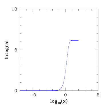
Figure 1: Plot of the integral $\int_{0}^{x_{i}}y\exp(-u_{i})du_{i}$ versus $x\equiv x_{1}$. The value changes quickly only near the moment of decay time, $t\sim\Gamma^{-1}$, and becomes constant afterwards.

3.4 Final curvature and isocurvature perturbations

After all the curvaton fields decay, i.e. $\Omega_{i}=0$, we are left with the overall curvature perturbation given by, from Eq. (20),

$$\zeta =\frac{\dot{\rho}_{\gamma}}{\dot{\rho}}\zeta_{\gamma}^{\mathrm{(out)}}+\frac{\dot{\rho}_{m}}{\dot{\rho}}\zeta_{m}^{\mathrm{(out)}}$$

$$=\frac{4\Omega_{\gamma}}{4\Omega_{\gamma}+3\Omega_{m}}\zeta_{\gamma}^{\mathrm{(out)}}+\frac{3\Omega_{m}}{4\Omega_{\gamma}+3\Omega_{m}}\zeta_{m}^{\mathrm{(out)}}\,.$$ (68)

The final matter and radiation curvature perturbations are constant on large scales and given by Eqs. (3.1) and (49), respectively. Their transfer coefficients are determined by Eqs. (3.1), (50) and (67). Thus, the isocurvature perturbation between matter and radiation components $\mathcal{S}_{m\gamma}=3(\zeta_{m}-\zeta_{\gamma})$, which is fixed after all the curvaton fields decay so that $\zeta_{\gamma}$ and $\zeta_{m}$ become constants, is written as

$$\mathcal{S}_{m\gamma}^{\mathrm{(out)}} =3\left(\zeta_{m}^{\mathrm{(out)}}-\zeta_{\gamma}^{\mathrm{(out)}}\right)$$

$$=3\sum_{i}(s_{i}-r_{i})\zeta_{i}^{\mathrm{(in)}}\,.$$ (69)

A particularly simple case is when all the decay rates are the same: then, from Eq. (3.1), the transfer coefficient of matter curvature perturbation becomes simply

$$s_{i}=\frac{\Omega_{i}^{\mathrm{(in)}}}{\sum_{j}\Omega_{j}^{\mathrm{(in)}}}=\frac{\Omega_{i}^{\mathrm{(in)}}}{1-\Omega_{\gamma}^{\mathrm{(in)}}}\,,$$ (70)

where we have assumed that initially there is no matter component. As can be seen clearly, the most significant contribution to the final matter curvature perturbation comes from the curvaton field which initially occupies the largest energy density among the curvatons. For $r_{i}$, we only need to consider a single moment of decay since the curvaton fields decay at the same time. Thus, from Eqs. (41) and (43), we simply have

$$f_{i}^{\mathrm{(dec)}}=\frac{3{\rho_{\gamma i}}/{\rho_{\gamma 0}}}{4+3\sum_{j}\rho_{\gamma j}/{\rho_{\gamma 0}}}\,,$$ (71)

and the final radiation curvature perturbation becomes, from Eq. (44),

$$\zeta_{\gamma}^{\mathrm{(out)}}=\left(1-\sum_{i}f_{i}^{\mathrm{(dec)}}\right)\zeta_{\gamma 0}^{\mathrm{(in)}}+\sum_{i}f_{i}^{\mathrm{(dec)}}\zeta_{i}^{\mathrm{(in)}}\,.$$ (72)

Now, from Eqs. (66) and (67), we can see that the ratio ${\rho_{\gamma i}}/{\rho_{\gamma 0}}$ is proportional to $\alpha_{i}$, which is again proportional to $\Omega_{i}^{\mathrm{(in)}}$, since [integral] $\equiv\int_{x_{0}}^{x_{i}}y\exp(-u_{i})du_{i}$ will have the same value as discussed in the previous section. Hence,

$$r_{i}=f_{i}^{\mathrm{(dec)}}=\frac{3\mathrm{[integral]}\alpha_{i}}{4+3\mathrm{[integral]}\sum_{j}\alpha_{j}}=\frac{3C\mathrm{[integral]}\Omega_{i}^{\mathrm{(in)}}}{4+3C\mathrm{[integral]}\sum_{j}\Omega_{j}^{\mathrm{(in)}}}\,,$$ (73)

where $C=\Gamma_{\gamma}{H^{\mathrm{(in)}}}^{1/2}/\left(\Gamma^{3/2}{\Omega_{\gamma}^{\mathrm{(in)}}}^{3/4}\right)$ is the common coefficient of proportionality of $\alpha_{i}$ to $\Omega_{i}^{\mathrm{(in)}}$. Thus, with one further assumption that the initial radiation curvature perturbation is negligible, i.e. $\zeta_{\gamma 0}^{\mathrm{(in)}}\approx 0$, the final isocurvature perturbation is, from Eq. (3.4),

$$\mathcal{S}_{m\gamma}^{\mathrm{(out)}}\approx 3\sum_{i}\left[\frac{1}{1-\Omega_{\gamma}^{\mathrm{(in)}}}-\frac{3C\mathrm{[integral]}}{4+3C\mathrm{[integral]}\left(1-\Omega_{\gamma}^{\mathrm{(in)}}\right)}\right]\Omega_{i}^{\mathrm{(in)}}\zeta_{i}^{\mathrm{(in)}}\,,$$ (74)

and thus the transfer from the initial curvature perturbation $\zeta_{i}^{\mathrm{(in)}}$ is proportional to the corresponding initial density fraction $\Omega_{i}^{\mathrm{(in)}}$.

4 Applications

In this section, we apply our analytic estimates obtained in the previous section to several examples and compare with numerical results.

4.1 Single curvaton

First we consider a simple example where a single curvaton field decays into radiation and matter with decay rates $\Gamma^{(1)}_{\gamma}$ and $\Gamma^{(1)}_{m}$, respectively. If we assume that the initial curvature perturbation in radiation is negligible, which is usually taken as the initial condition for the curvaton scenario, the radiation curvature perturbation after curvaton decay is purely due to the decay of the curvaton field and from Eqs. (49) is given by

$$\begin{split}\zeta_{\gamma}^{\mathrm{(out)}}\approx f_{1}^{\mathrm{(dec)}}\zeta_{1}^{\mathrm{(in)}}\,,\end{split}$$ (75)

where

$$\begin{split}f_{1}^{\mathrm{(dec)}}=\frac{3\rho_{\gamma 1}/{\rho_{\gamma 0}}}{4+3\rho_{\gamma 1}/{\rho_{\gamma 0}}}\,.\end{split}$$ (76)

As discussed in the previous sections this is constant after the curvaton decay, and is completely determined once we find the ratio $\rho_{\gamma 1}/{\rho_{\gamma 0}}$. This ratio is given by Eq. (67) as

$$\begin{split}\frac{\rho_{\gamma 1}}{{\rho_{\gamma 0}}}&=\alpha_{1}\int_{x_{0}}^{x_{1}}y(u_{1})e^{-u_{1}}du_{1}\,,\end{split}$$ (77)

and depends only on $x_{H}$ and $\alpha_{1}$ given by Eqs. (63) and (66), respectively.

If initially radiation dominates, i.e. $\Omega_{\gamma 0}^{\mathrm{(in)}}\approx 1$, we find that

$$x_{H} \approx\frac{\Gamma^{(1)}}{H^{\mathrm{(in)}}}\,,$$ (78)

$$\alpha_{1} \approx\Omega_{1}^{\mathrm{(in)}}\frac{\Gamma_{\gamma}^{(1)}}{\Gamma^{(1)}}\left(\frac{\Gamma^{(1)}}{H^{\mathrm{(in)}}}\right)^{-1/2}$$ (79)

where $\alpha_{1}$ becomes identical with $p$ of Ref. [18] in the limit $\Gamma_{\gamma}^{(1)}\gg\Gamma_{m}^{(1)}$. In this case since the universe is dominated by radiation component, $a\propto t^{1/2}$ and $H=(2t)^{-1}$. That is, for small $x_{1}$ the solution of Eq. (65) is given by

$$\begin{split}y(x_{1})=(2x_{1})^{1/2}\,,\end{split}$$ (80)

with $x_{1}^{\mathrm{(in)}}=x_{H}/2$, and we can see that $y(x_{1})$ is independent of $x_{H}$ [21]. Thus the curvature perturbation depends only on $\alpha_{1}$, which is shown by using the phase space plot in Refs. [17, 18].

Furthermore, in the case that the curvaton does not dominate the density during the evolution, we can further approximate Eq. (77) analytically. From the sudden decay approximation, we can see that $\alpha_{1}+\beta_{1}\approx\Omega_{1}^{\mathrm{(in)}}(\Gamma^{(1)}/H^{\mathrm{(in)}})^{-1/2}\ll 1$ guarantees the radiation domination [17], thus using $y(t)\simeq x_{H}^{1/2}(t/t_{0})^{1/2}$, we obtain

$$\frac{\rho_{\gamma 1}}{{\rho_{\gamma 0}}} \approx\alpha_{1}x_{H}^{1/2}\int_{x_{0}}^{x_{1}}\left(\frac{t}{t_{0}}\right)^{1/2}e^{-u_{1}}du_{1}$$

$$=\frac{\alpha_{1}x_{H}^{1/2}}{\sqrt{t_{0}\Gamma^{(1)}}}\int_{x_{0}}^{x_{1}}u_{1}^{1/2}e^{-u_{1}}du_{1}$$

$$\approx\sqrt{2}\alpha_{1}\int_{x_{0}}^{x_{1}}u_{1}^{1/2}e^{-u_{1}}du_{1}\,,$$ (81)

where we have used Eqs. (78) and (79) and $t_{0}=1/\left(2H^{\mathrm{(in)}}\right)$ for the last equality. Now let us take a look at the integral: it is integrated from the initial time to some later time after the curvaton field decays. Since we are free to choose the initial time and the integrand is suppressed at later times after the curvaton decay, we can take the range of integration from zero to infinity without loss of generality. Then the integral becomes just $\Gamma(3/2)=\sqrt{\pi}/2$. Hence,

$$\frac{\rho_{\gamma 1}}{{\rho_{\gamma 0}}}=\sqrt{\frac{\pi}{2}}\alpha_{1}\approx 1.25331\alpha_{1}\,.$$ (82)

Therefore from Eqs. (75), (76) and (82), the final curvature perturbation $\zeta_{\gamma}^{\mathrm{(out)}}$ after the curvaton decays is

$$\begin{split}\zeta_{\gamma}^{\mathrm{(out)}}\approx\frac{3}{4}\sqrt{\frac{\pi}{2}}\alpha_{1}\zeta_{1}^{\mathrm{(in)}}\approx 0.939986\ \alpha_{1}\zeta_{1}^{\mathrm{(in)}}\,,\end{split}$$ (83)

which is in good agreement with Ref. [18].

In the opposite limit ($\alpha_{1}+\beta_{1}\gg 1$), i.e. the curvaton field completely dominates the energy density of the universe before it decays, mostly the region of integration is the matter dominated epoch, thus $a\propto t^{2/3}$. We can find the time of the transition from radiation dominated to curvaton dominated era ($\Omega_{\gamma 0}=\Omega_{1}$) from sudden decay approximation,

$$\begin{split}t_{tr}\approx\frac{1}{2H^{\mathrm{(in)}}}\left(\frac{\Omega_{\gamma 0}^{\mathrm{(in)}}}{\Omega_{1}^{\mathrm{(in)}}}\right)^{2}.\end{split}$$ (84)

Using this , the integral becomes

$$\begin{split}\frac{\rho_{\gamma 1}}{{\rho_{\gamma 0}}}&\approx\alpha_{1}x_{H}^{1/2}\left[\int_{x_{0}}^{x_{tr}}\left(\frac{t}{t_{0}}\right)^{1/2}e^{-u_{1}}du_{1}+\left(\frac{t_{tr}}{t_{0}}\right)^{1/2}\int_{x_{tr}}^{x_{1}}\left(\frac{t}{t_{tr}}\right)^{2/3}e^{-u_{1}}du_{1}\right],\end{split}$$ (85)

where $x_{tr}=\Gamma t_{tr}$. Ignoring the contribution from the transient radiation dominated era, we find

$$\frac{\rho_{\gamma 1}}{{\rho_{\gamma 0}}} \approx\alpha_{1}x_{H}^{1/2}\left(\frac{t_{tr}}{t_{0}}\right)^{1/2}\int_{x_{0}}^{x_{1}}\left(\frac{t}{t_{tr}}\right)^{2/3}e^{-u_{1}}du_{1}$$

$$\approx 2^{2/3}\alpha_{1}\left[\frac{\Gamma^{(1)}}{H^{\mathrm{(in)}}}\left(\frac{\Omega_{\gamma 0}^{\mathrm{(in)}}}{\Omega_{1}^{\mathrm{(in)}}}\right)^{2}\right]^{-1/6}\int_{0}^{\infty}u_{1}^{2/3}e^{-u_{1}}du_{1}$$

$$\approx 2^{2/3}\Gamma\left(\frac{5}{3}\right)\left(\alpha_{1}+\beta_{1}\right)^{1/3}\alpha_{1}$$

$$\approx 1.43302\left(\alpha_{1}+\beta_{1}\right)^{1/3}\alpha_{1}\,,$$ (86)

where we assume that initially radiation dominates the universe so that $x_{H}\approx\Gamma^{(1)}/H^{\mathrm{(in)}}$ and $t_{0}\approx 1/(2H^{\mathrm{(in)}})$.

For the final matter curvature perturbation, assuming that initially there is no matter component, it is independent of the curvaton domination and is simply given from Eqs. (3.1) and (3.1) by

$$\zeta_{m}^{\mathrm{(out)}}=\zeta_{1}^{\mathrm{(in)}}\,,$$ (87)

i.e. it is just the same as the initial curvature perturbation in the curvaton, as shown in Ref. [18].

4.2 Two curvatons

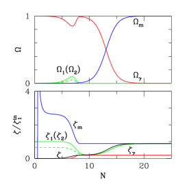
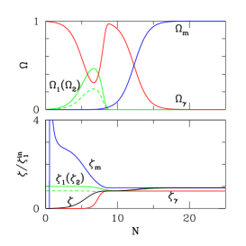
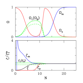
Figure 2: The evolution of density parameters (upper row) and curvature perturbations (lower row) for three cases of two curvaton decays: as shown, the energy densities of the two curvaton fields are sub-dominant (left panel), dominant (right panel) and comparable (middle panel) to the radiation energy density. The details are given in Table 1.

		left panel	middle panel	right panel
$\zeta_{2}^{{\mathrm{(in)}}}/\zeta_{1}^{\mathrm{(in)}}$		0.65	0.8	0.75
$\Gamma_{\gamma}^{(1)}/H^{\mathrm{(in)}}$		$10^{-6}$	$10^{-6}$	$10^{-8}$
$\Gamma_{\gamma}^{(2)}/H^{\mathrm{(in)}}$		$10^{-6}$	$10^{-6}$	$10^{-8}$
$\Gamma_{m}^{(1)}/H^{\mathrm{(in)}}$		$10^{-8}$	$10^{-8}$	$10^{-10}$
$\Gamma_{m}^{(2)}/H^{\mathrm{(in)}}$		$10^{-8}$	$10^{-8}$	$10^{-10}$
$\Omega_{1}^{\mathrm{(in)}}$		$10^{-3.7}$	$10^{-2.5}$	$10^{-2.0}$
$\Omega_{2}^{\mathrm{(in)}}$		$10^{-4.0}$	$10^{-2.8}$	$10^{-2.1}$
$r_{1}$	analytic approx.	0.151008	0.582546	0.556639
	analytic limit	0.144650	-	0.575484
$r_{2}$	analytic approx.	0.0756833	0.291964	0.442155
	analytic limit	0.0724969	-	0.423350
$\zeta_{\gamma}^{\mathrm{(out)}}/\zeta_{1}^{\mathrm{(in)}}$	analytic approx.	0.200202	0.816117	0.888255
	analytic limit	0.191773	-	0.892997
	numerical	0.195615	0.792049	0.887648
$s_{1}$	analytic	0.666139	0.666139	0.557312
$s_{2}$	analytic	0.333861	0.333861	0.442688
$\zeta_{m}^{\mathrm{(out)}}/\zeta_{1}^{\mathrm{(in)}}$	analytic	0.883149	0.933227	0.889327
	numerical	0.883149	0.933228	0.889328

Table 1: The analytic and numerical results for the cases shown in Fig. 2. In the upper half of the table, we give the initial values used in the calculation and in the lower half we compare the analytic estimates with the numerical results. For analytic approximation we first solved Eq. (65) to find the density ratio Eq. (67) and then used Eqs. (48), (49) and (50). For analytic limit we use Eqs. (82) and (4.1) to find the radiation ratio in the both limits where the curvaton fields remain sub-dominant / dominant. For final matter curvature perturbation we have used Eqs. (3.1) and (3.1) for analytic estimate. Note that in the middle panel we did not use any of the analytic limits, since in this case the curvatons fields occupy an amount of energy density comparable to radiation and does not correspond to any of the limiting cases.

In this section we consider the next simplest case where there are two curvaton fields decaying into both radiation and matter. If we assume again that the initial curvature perturbation in radiation is negligible, the final curvature perturbation in radiation is, from Eq. (49),

$$\zeta_{\gamma}^{\mathrm{(out)}} =r_{1}\zeta_{1}^{\mathrm{(in)}}+r_{2}\zeta_{2}^{\mathrm{(in)}}$$

$$=\left(1-f_{2}^{\mathrm{(dec)}}\right)f_{1}^{\mathrm{(dec)}}\zeta_{1}^{\mathrm{(in)}}+f_{2}^{\mathrm{(dec)}}\zeta_{2}^{\mathrm{(in)}}\,,$$ (88)

where

$$f_{1}^{\mathrm{(dec)}} =\frac{3\rho_{\gamma 1}/{\rho_{\gamma 0}}}{4+3\rho_{\gamma 1}/{\rho_{\gamma 0}}}\,,$$

$$f_{2}^{\mathrm{(dec)}} =\frac{3\rho_{\gamma 2}/{\rho_{\gamma 0}}}{4\left(1+\rho_{\gamma 1}/{\rho_{\gamma 0}}\right)+3\rho_{\gamma 2}/{\rho_{\gamma 0}}}\,.$$ (89)

The final curvature perturbation in matter is given by, from Eq. (3.1),

$$\zeta_{m}^{\mathrm{(out)}} =s_{1}\zeta_{1}^{\mathrm{(in)}}+s_{2}\zeta_{2}^{\mathrm{(in)}}$$

$$=\frac{\beta_{1}}{\beta_{1}+\beta_{2}}\zeta_{1}^{\mathrm{(in)}}+\frac{\beta_{2}}{\beta_{1}+\beta_{2}}\zeta_{2}^{\mathrm{(in)}}\,,$$ (90)

Therefore the final isocurvature perturbation between radiation and matter is now completely determined from Eq. (3.4). In Fig. 2, we show some examples where two curvaton fields decay into radiation and matter.

If the energy density of the curvaton fields remains sub-dominant throughout the evolution of the universe, which would be guaranteed by the conditions

$$\begin{split}\alpha_{1}+\beta_{1}\ll 1,\quad\alpha_{2}+\beta_{2}\ll 1,\end{split}$$ (91)

then

$$f_{1}^{\mathrm{(dec)}} \approx c_{R}\alpha_{1}\,,$$

$$f_{2}^{\mathrm{(dec)}} \approx c_{R}\alpha_{2}\,.$$ (92)

where $c_{R}=3\sqrt{\pi/2}/4\approx 0.939986$.

Now it is clear that the transfer coefficients are proportional to the initial density parameter of the corresponding curvaton fields. Thus with sub-dominant curvatons the isocurvature perturbation is

$$\mathcal{S}_{m\gamma}^{\mathrm{(out)}} =3\sum_{i}(s_{i}-r_{i})\zeta_{i}^{\mathrm{(in)}}$$

$$\approx 3\left[\left(\frac{\beta_{1}}{\beta_{1}+\beta_{2}}-c_{R}\alpha_{1}\right)\zeta_{1}^{\mathrm{(in)}}+\left(\frac{\beta_{2}}{\beta_{1}+\beta_{2}}-c_{R}\alpha_{1}\right)\zeta_{2}^{\mathrm{(in)}}\right]\,.$$ (93)

For the curvaton dominated case before they decay, we can take similar steps as radiation dominated one. For example in the case of the right panel of Fig. 2, the transfer coefficients of the matter curvature perturbation $s_{i}$ are

$$\begin{split}s_{1(2)}=\frac{\alpha_{1(2)}}{\alpha_{1}+\alpha_{2}}\,,\end{split}$$ (94)

where we have used $\Gamma_{m}^{(1)}/\Gamma^{(1)}=\Gamma_{m}^{(2)}/\Gamma^{(2)}$. Since the two curvatons dominate at the same epoch, we can use the same normalisation for $y$-function, thus $f_{1}$ and $f_{2}$ are easily approximated as

$$\begin{split}f_{1}\approx 1\,,\qquad f_{2}\approx\frac{\alpha_{1}}{\alpha_{1}+\alpha_{2}}=\frac{\Omega_{1}}{\Omega_{1}+\Omega_{2}}\,,\end{split}$$ (95)

where in the last equality we have used $\Gamma_{\gamma}^{(1)}/\Gamma^{(1)}=\Gamma_{\gamma}^{(2)}/\Gamma^{(2)}$. The transfer coefficients of the radiation curvature perturbation $r_{i}$ are

$$\begin{split}r_{1(2)}=\frac{\alpha_{1(2)}}{\alpha_{1}+\alpha_{2}}\,.\end{split}$$ (96)

The isocurvature perturbation hence almost vanishes, which is shown in the right panel of Fig. 2.

4.3 Multiple curvatons

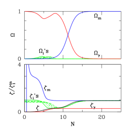
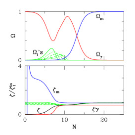
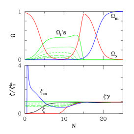
Figure 3: The same as Fig. 2 but with five curvaton fields. The details of the parameters are given in Table 2.

		left panel	middle panel	right panel
$\zeta_{i}^{{\mathrm{(in)}}}/\zeta_{1}^{\mathrm{(in)}}$		$(1.0,0.95,0.9,0.85,0.8)$	$(1.0,0.95,0.9,0.85,0.8)$	$(0.6,0.7,0.8,0.9,1.0)$
$\log_{10}\left(\Gamma_{\gamma}^{(i)}/H^{\mathrm{(in)}}\right)$		$(-4,-4.5,-5,-5.5,-6)$	$(-6,-6.5,-7,-7.5,-8)$	$(-8,-8.5,-9,-9.5,-10)$
$\log_{10}\left(\Gamma_{m}^{(i)}/H^{\mathrm{(in)}}\right)$		$(-6,-6.5,-7,-7.5,-8)$	$(-8,-8.5,-9,-9.5,-10)$	$(-10,-10.5,-11,-11.5,-12)$
$\log_{10}\left(\Omega_{i}^{\mathrm{(in)}}\right)$		$(-3,-3.25,-3.5,-3.75,-4)$	$(-3,-3.25,-3.5,-3.75,-4)$	$(-3,-2.75,-2.5,-2.25,-2)$
$r_{1}$	analytic approx.	0.0656799	0.187597	0.00900859
	analytic limit	0.0642904	-	0.00406052
$r_{2}$	analytic approx.	0.0650727	0.172502	0.0256607
	analytic limit	0.0625240	-	0.0142846
$r_{3}$	analytic approx.	0.0646559	0.166930	0.0768897
	analytic limit	0.0609761	-	0.0527442
$r_{4}$	analytic approx.	0.0642456	0.163447	0.228450
	analytic limit	0.0596027	-	0.196372
$r_{5}$	analytic approx.	0.0637326	0.160106	0.659821
	analytic limit	0.0583711	-	0.732362
$\zeta_{\gamma}^{\mathrm{(out)}}/\zeta_{1}^{\mathrm{(in)}}$	analytic approx.	0.291284	0.768726	0.950306
	analytic limit	0.275926	-	0.963727
	numerical	0.291515	0.765150	0.956406
$\zeta_{m}^{\mathrm{(out)}}/\zeta_{1}^{\mathrm{(in)}}$	analytic	0.950652	0.950652	0.901304
	numerical	0.950670	0.950652	0.901304

Table 2: The analytic and numerical results of in Fig. 3. As in Table 1, we show the initial parameters in the upper half.

Now we consider more general case where there exist a number of curvaton fields decaying into radiation and matter. It is straightforward to extract the final curvature perturbations either numerically by solving Eqs. (14)–(17) and (25)–(27), or analytically by using Eqs (3.4) with Eqs. (3.1) and (49). Indeed, as shown in Table 2, analytic estimates give good approximations to the full numerical result within an error of 0.7% (5%) with analytic approximation (analytic limit). However the evolution of each perturbation could be quite non-trivial, as shown in Fig. 3 where we have plotted several cases with five curvaton fields. We can read the followings:

• The evolution of the total curvature perturbation $\zeta$ depends, not surprisingly, on which component dominates the energy density of the universe. During the curvaton fields dominates the energy density before they decay, $\zeta$ is the average of $\zeta_{i}$’s and constantly evolving during this epoch, since the curvatons are decaying into radiation and matter. This is clearly seen in the right panel of Fig. 3. After all the curvatons decay, $\zeta$ follows $\zeta_{\gamma}$ when radiation dominates before matter begins to dominate, and $\zeta=\zeta_{m}$ afterwards, as shown in Eq. (3.4).

• $\zeta_{\gamma}$ and $\zeta_{m}$ evolve only during the curvaton fields decay and remain constant after curvaton fields decay since, as mentioned before, there is no energy transfer between radiation and matter. Especially, since matter is assumed to be produced purely due to the decay of the curvatons, $\zeta_{m}$ is greatly affected no matter the curvaton fields dominate the energy density before decay or not, e.g. in the left panel of Fig. 3 where the curvatons never contribute significantly, their impact on $\zeta_{m}$ is large: when $\rho_{m0}=0$, $\zeta_{m}$ is just a weighted sum of the initial curvature perturbations of the curvatons and the weight $s_{i}$ is basically the ratio of the corresponding curvaton energy density multiplied by the branching ratio to matter to the total curvaton energy density responsible to matter density, as shown in Eq. (3.1). For $\zeta_{\gamma}$, it is noticeable that $\zeta_{\gamma}$ becomes significant only when the curvaton fields occupy significant fraction of total energy density before they decay, as can be compared between different columns of Fig. 3. This is because practically the radiation is completely generated by the decay of curvaton fields, making the pre-existing radiation irrelevant.

• From the discussion above, one may tempted to conclude that there will be negligible isocurvature perturbation between matter and radiation if the curvatons dominate before they decay, because they are both generated due to the decay of the curvaton fields. This is not true when there are a number of curvaton fields: the final isocurvature perturbation is dependent on the background parameters such as curvaton densities and decay rates. For example, in Fig. 4, the branching ratio to matter of the curvaton $\sigma_{5}$ which has the largest energy density is extremely small, i.e.

  $$\frac{\Gamma_{m}^{(5)}}{\sqrt{\Gamma^{(5)}}}\approx 10^{-16}\,.$$ (97)

  Thus, although $\zeta_{m}$ receives contribution from the decay product of the curvaton with large energy density and this gives a rise of $\zeta_{m}$, this rise is never enough to catch up $\zeta_{\gamma}$ to make $\mathcal{S}_{m\gamma}^{\mathrm{(out)}}$ vanishing if the branching ratio is very small as in this case. This is reminiscent of multi-field inflation: in multi-field inflation, there is no unique prediction on the isocurvature perturbation produced during inflation. The detail depends on the inflaton trajectory in the field space. Likewise, generally we can hardly make any definite prediction on the isocurvature perturbation without the detail.

Figure 4: All the parameters are the same as the right panel of Fig. 3 except the branching ratios to matter: here, $\Gamma_{i}^{(m)}/H^{\mathrm{(in)}}$ is given by $10^{-19}$, $10^{-17.5}$, $10^{-15}$, $10^{-13.5}$ and $10^{-11}$ for each curvaton, respectively. In this case, we have $\zeta_{\gamma}^{\mathrm{(out)}}/\zeta_{1}^{\mathrm{(in)}}=0.956524$ ($\zeta_{\gamma}^{\mathrm{(out)}}/\zeta_{1}^{\mathrm{(in)}}=0.950257$ with analytic approx.) and $\zeta_{m}^{\mathrm{(out)}}/\zeta_{1}^{\mathrm{(in)}}=0.602384$, making $\mathcal{S}_{m\gamma}^{\mathrm{(out)}}$ not negligible.

5 Conclusions

In this paper, we have studied the evolution of the universe which contains a number of non-interacting scalar particles (the “curvatons” $\sigma_{i}$) decaying into radiation ($\gamma$) and pressureless matter ($m$) after inflation. We first have written the evolution equations of the background densities of the components $\rho_{i}$, $\rho_{\gamma}$ and $\rho_{m}$ which compose the universe and of the curvature perturbations of corresponding component $\zeta_{i}$ $\zeta_{\gamma}$ and $\zeta_{m}$ on flat hypersurfaces, Eqs. (14)–(17) and (25)–(27). These equations can be numerically solved and give the resulting curvature perturbations of the components, as well as the total curvature perturbation $\zeta$ given by Eq. (20).

Using the sudden decay approximation, we have obtained analytic estimates of the final radiation and matter curvature perturbations $\zeta_{\gamma}^{\mathrm{(out)}}$ and $\zeta_{m}^{\mathrm{(out)}}$ which are in good agreement with full numerical results. With the composite densities $\widetilde{\rho}_{\gamma i}$ and $\widetilde{\rho}_{mi}$, given by Eq. (3), we can relate $\zeta_{\gamma}^{\mathrm{(out)}}$ and $\zeta_{m}^{\mathrm{(out)}}$ to the initial curvature perturbations associated with the curvatons $\zeta_{i}^{\mathrm{(in)}}$: the curvature perturbation $\widetilde{\zeta}_{mi}$ is conserved and hence the final matter curvature perturbation $\zeta_{m}^{\mathrm{(out)}}$ has very simple relation to $\zeta_{i}^{\mathrm{(in)}}$ Eq. (3.1) with the transfer coefficient $s_{i}$ given by Eq. (3.1). Meanwhile, $\widetilde{\zeta}_{\gamma i}$ is not constant on large scales since the equation of state of $\widetilde{\rho}_{\gamma i}$ is not unique. Nevertheless, we can find that $\zeta_{\gamma}^{\mathrm{(out)}}$ is written in terms of $\zeta_{i}^{\mathrm{(in)}}$ as Eq. (49), with the transfer coefficient $r_{i}$ given by Eq. (50). $r_{i}$ is determined once the ratio $\rho_{\gamma i}/\rho_{\gamma 0}$ is found, and we have found a general and model independent result Eq. (67). This might be also useful to investigate non-Gaussianity of the primordial curvature perturbation in the multi curvaton scenario [22].

We have applied our results to several different cases. The analytic estimates give good enough fits to the full numerical results, within an error of $\mathcal{O}(0.1)$%. When the curvatons dominate the energy density of the universe before they decay, the final radiation curvature perturbation $\zeta_{\gamma}^{\mathrm{(out)}}$ is significantly affected by the curvature perturbations of the curvatons $\zeta_{i}$, since practically radiation is generated by the decay of the curvaton fields and the pre-existing radiation is irrelevant. More importantly, the isocurvature perturbation between matter and radiation given by Eq. (3.4) depends on the detailed decay rate of the curvatons: for example, in the right panel of Fig. 2, $\zeta_{\gamma}^{\mathrm{(out)}}$ and $\zeta_{m}^{\mathrm{(out)}}$ are of almost the same amplitudes and thus isocurvature perturbation is highly suppressed. However, as shown in Fig. 4, when the branching ratios to matter are different for different curvatons, we may have significant isocurvature perturbation depending on the initial values of the background quantities. We can determine $\mathcal{S}_{m\gamma}^{\mathrm{(out)}}$ which may be detected in the CMB observations only when we have detailed information on the curvaton fields.

- [1] M. Tegmark et al. [SDSS Collaboration], “Cosmological parameters from SDSS and WMAP,” Phys. Rev. D 69, 103501 (2004) [arXiv:astro-ph/0310723] ; U. Seljak et al. [SDSS Collaboration], “Cosmological parameter analysis including SDSS Ly-alpha forest and galaxy bias: Constraints on the primordial spectrum of fluctuations, neutrino mass, and dark energy,” Phys. Rev. D 71, 103515 (2005) [arXiv:astro-ph/0407372] ; D. N. Spergel et al. [WMAP Collaboration], “Wilkinson Microwave Anisotropy Probe (WMAP) three year results: Implications for cosmology,” arXiv:astro-ph/0603449.
- [2] A. H. Guth, “The inflationary universe: A possible solution to the horizon and flatness problems,” Phys. Rev. D 23, 347 (1981) ; A. D. Linde, “A new inflationary universe scenario: A possible solution of the horizon, flatness, homogeneity, isotropy and primordial monopole problems,” Phys. Lett. B 108, 389 (1982) ; A. Albrecht and P. J. Steinhardt, “Cosmology for grand unified theories with radiatively induced symmetry breaking,” Phys. Rev. Lett. 48, 1220 (1982).
- [3] J. M. Bardeen, P. J. Steinhardt and M. S. Turner, “Spontaneous creation of almost scale - free density perturbations in an inflationary universe,” Phys. Rev. D 28 (1983) 679.
- [4] J. O. Gong and E. D. Stewart, “The density perturbation power spectrum to second-order corrections in the slow-roll expansion,” Phys. Lett. B 510, 1 (2001) [arXiv:astro-ph/0101225] ; J. Choe, J. O. Gong and E. D. Stewart, “Second order general slow-roll power spectrum,” JCAP 0407, 012 (2004) [arXiv:hep-ph/0405155].
- [5] A. A. Starobinsky, “Multicomponent de Sitter (inflationary) stages and the generation of perturbations,” JETP Lett. 42 (1985) 152 [Pisma Zh. Eksp. Teor. Fiz. 42 (1985) 124] ; M. Sasaki and E. D. Stewart, “A General analytic formula for the spectral index of the density perturbations produced during inflation,” Prog. Theor. Phys. 95, 71 (1996) [arXiv:astro-ph/9507001] ; M. Sasaki and T. Tanaka, “Super-horizon scale dynamics of multi-scalar inflation,” Prog. Theor. Phys. 99, 763 (1998) [arXiv:gr-qc/9801017] ; J. O. Gong and E. D. Stewart, “The power spectrum for a multi-component inflaton to second-order corrections in the slow-roll expansion,” Phys. Lett. B 538, 213 (2002) [arXiv:astro-ph/0202098].
- [6] D. Wands, K. A. Malik, D. H. Lyth and A. R. Liddle, “A new approach to the evolution of cosmological perturbations on large scales,” Phys. Rev. D 62, 043527 (2000) [arXiv:astro-ph/0003278].
- [7] A. R. Liddle and D. H. Lyth, “Cosmological inflation and large-scale structure,” Cambridge, UK: Univ. Pr. (2000) 400 p ; V. Mukhanov, “Physical foundations of cosmology,” Cambridge, UK: Univ. Pr. (2005) 421 p
- [8] M. Y. Khlopov, “Cosmoparticle physics,” Singapore, Singapore: World Scientific (1999) 577 p
- [9] D. H. Lyth and D. Wands, “Generating the curvature perturbation without an inflaton,” Phys. Lett. B 524, 5 (2002) [arXiv:hep-ph/0110002] ; T. Moroi and T. Takahashi, “Effects of cosmological moduli fields on cosmic microwave background,” Phys. Lett. B 522, 215 (2001) [Erratum-ibid. B 539, 303 (2002)] [arXiv:hep-ph/0110096].
- [10] D. H. Lyth, “Can the curvaton paradigm accommodate a low inflation scale,” Phys. Lett. B 579, 239 (2004) [arXiv:hep-th/0308110] ; T. Moroi and T. Takahashi, “Cosmic density perturbations from late-decaying scalar condensations,” Phys. Rev. D 66, 063501 (2002) [arXiv:hep-ph/0206026] ; J. O. Gong, “Modular thermal inflation without slow-roll approximation,” Phys. Lett. B 637, 149 (2006) [arXiv:hep-ph/0602106].
- [11] J. O. Gong, in preparation.
- [12] S. Dimopoulos, S. Kachru, J. McGreevy and J. G. Wacker, “N-flation,” arXiv:hep-th/0507205.
- [13] J. O. Gong, “End of multi-field inflation and the perturbation spectrum,” Phys. Rev. D 75, 043502 (2007) [arXiv:hep-th/0611293].
- [14] A. R. Liddle, A. Mazumdar and F. E. Schunck, “Assisted inflation,” Phys. Rev. D 58, 061301 (1998) [arXiv:astro-ph/9804177] ; P. Kanti and K. A. Olive, “On the realization of assisted inflation,” Phys. Rev. D 60, 043502 (1999) [arXiv:hep-ph/9903524].
- [15] M. Lemoine and J. Martin, “Neutralino dark matter and the curvaton,” Phys. Rev. D 75, 063504 (2007) [arXiv:astro-ph/0611948].
- [16] H. Kodama and M. Sasaki, “Cosmological perturbation theory,” Prog. Theor. Phys. Suppl. 78 (1984) 1.
- [17] K. A. Malik, D. Wands and C. Ungarelli, “Large-scale curvature and entropy perturbations for multiple interacting fluids,” Phys. Rev. D 67 (2003) 063516 [arXiv:astro-ph/0211602].
- [18] S. Gupta, K. A. Malik and D. Wands, “Curvature and isocurvature perturbations in a three-fluid model of curvaton decay,” Phys. Rev. D 69 (2004) 063513 [arXiv:astro-ph/0311562].
- [19] D. H. Lyth, C. Ungarelli and D. Wands, “The primordial density perturbation in the curvaton scenario,” Phys. Rev. D 67, 023503 (2003) [arXiv:astro-ph/0208055].
- [20] K. Hamaguchi, M. Kawasaki, T. Moroi and F. Takahashi, “Curvatons in supersymmetric models,” Phys. Rev. D 69 (2004) 063504 [arXiv:hep-ph/0308174].
- [21] R. J. Scherrer and M. S. Turner, “Decaying particles do not heat up the universe,” Phys. Rev. D 31 (1985) 681.
- [22] M. Sasaki, J. Valiviita and D. Wands, “Non-gaussianity of the primordial perturbation in the curvaton model,” Phys. Rev. D 74 (2006) 103003 [arXiv:astro-ph/0607627]; J. Valiviita, M. Sasaki and D. Wands, “Non-Gaussianity and constraints for the variance of perturbations in the curvaton model,” arXiv:astro-ph/0610001.