On the detectability of non-trivial topologies

Abstract

We explore the main physical processes which potentially affect the topological signal in the Cosmic Microwave Background (CMB) for a range of toroidal universes. We consider specifically reionisation, the integrated Sachs-Wolfe (ISW) effect, the size of the causal horizon, topological defects and primordial gravitational waves. We use three estimators: the information content, the S/N statistic and the Bayesian evidence. While reionisation has nearly no effect on the estimators, we show that taking into account the ISW strongly decreases our ability to detect the topological signal. We also study the impact of varying the relevant cosmological parameters within the $2\sigma$ ranges allowed by present data. We find that only $\Omega_{\Lambda}$, which influences both ISW and the size of the causal horizon, significantly alters the detection for all three estimators considered here.

I Introduction

One of the fundamental questions of cosmology is whether the universe is infinite or finite, a question which is especially relevant in the context of string theory where several dimensions may be compact. With the move towards precision cosmology, it has become possible to study the topology of the universe up to the causal horizon which fundamentally limits our view of the world.

Many tests have recently been developed to detect and constrain the topology of the universe, see Refs. rep1 ; rep2 and references therein. Observationally a non-trivial topology can be detected directly with the observed map of CMB temperature and polarisation fluctuations through matched and correlated circles in the CMB circle ; cornish2 ; roukema ; luminet ; cress ; riap . The topology can also be searched for in the expansion of the CMB map in terms of spherical harmonics, $T(x)=\sum_{\ell,m}a_{\ell m}Y_{\ell m}(x)$, where $x$ are the pixels and both the temperature field and the $a_{\ell m}$ are random variables. The presence of a non-trivial topology introduces preferred directions, which breaks global isotropy and induces correlations between off-diagonal elements of the two-point correlation matrix $\left<a_{\ell m}a_{\ell^{\prime}m^{\prime}}^{*}\right>$. Methods to find such off-diagonal correlations and to put optimal constraints on the size of the universe were proposed in Ref. topo1 . They are based on matching the measured correlations to a given correlation matrix through a correlation coefficient, as well as a maximum likelihood method and Bayesian model comparison.

So far the focus was purely on trying to detect any non-trivial topologies. However, to determine reliable limits, it is also necessary to understand all effects which can affect the detection. For this purpose, we study the impact of changing the cosmological parameters in the ranges allowed by present data. This should be seen as a step towards a rigorous search for the presence of signs of non-trivial topologies in the CMB. Eventually, such an analysis should account for other contributions like foreground emissions as well as sky cuts.

One additional reason to perform such a detailed analysis comes from statistics. The potentially most direct way to quantify the probability that our universe is infinite is to compute the model probability with Bayesian evidence. To do this, one needs to integrate over all parameters, which means that one needs to know the behaviour of the likelihood for a topology under changes of the parameters.

This paper is organised as follows: we start by reviewing our notation and the likelihood-based probes of topology. We then study the main physical effects that are relevant for topology studies. Finally we discuss how changes in the cosmological parameters affect our detection ability, and what this means for realistic universes where the parameters are not known with absolute certainty.

II Methodology

In this section, all the simulations (as described in Refs. riaz1 ; riaz2 ) are based on a flat $\Lambda$CDM model with $\Omega_{\Lambda}=0.7$, a reduced Hubble parameter of $h=0.01H_{0}\times(1\;{\mathrm{km}}\;{\mathrm{s}^{-1}}\;{\mathrm{Mpc}^{-1}})^{-1}=0.67$, a Harrison-Zel’dovich initial power spectrum ($n_{\rm S}=1$) and a baryon density of $\Omega_{b}h^{2}=0.019$. With this choice of cosmological parameters we find a Hubble radius $c/H_{0}\approx 4.8\;{\mathrm{Gpc}}$, while the radius of the particle horizon is $R_{\rm h}\approx 15.6\;{\mathrm{Gpc}}$. In this paper we limit ourselves to cubic tori, denoted as T[X,X,X] where X is the size of the fundamental domain, in units of the Hubble radius. As an example, T[4,4,4] is a cubic torus of size $(19.3\;{\mathrm{Gpc}})^{3}$. The volume of such a torus is nearly half that of the observable universe. The diameter of the particle horizon is about $6.5c/H_{0}$ (cf. section III.1). We will focus on three different sizes, T[2,2,2], T[4,4,4] and T[6,6,6]. We combine the $\ell$ and $m$ indices of the spherical harmonic coefficients to a single index $s\equiv\ell(\ell+1)+m$ and mix both notations frequently.

In this paper we use the likelihood based methods of Ref. topo1 , which we review here quickly. The CMB likelihood is taken to be a multivariate Gaussian distribution with covariance matrix ${\cal B}_{ss^{\prime}}=\langle a_{s}^{*}a_{s^{\prime}}\rangle$ and zero mean, $\langle a_{s}\rangle=0$. This covariance matrix provides the full statistical description of the CMB for a given topology. The likelihood function then is

$${\cal L}({\cal B})\equiv p(a_{\ell m}|{\cal B})\propto\frac{1}{\sqrt{|{\cal B}|}}\exp\left\{-\frac{1}{2}\sum_{s,s^{\prime}}a^{*}_{s}{\cal B}^{-1}_{ss^{\prime}}a_{s^{\prime}}\right\},$$ (1)

where $|{\cal B}|$ is the determinant of the matrix ${\cal B}$. Any further model assumptions like the values of the cosmological parameters are implicitly included in the choice of ${\cal B}$.

Often it is easier to consider the logarithm of the likelihood, $\ln{\cal L}=-1/2(\ln|{\cal B}|+\chi^{2}+s_{\rm max}\ln(2\pi))$ where we have defined

$$\chi^{2}=\sum_{s,s^{\prime}}a^{*}_{s}{\cal B}^{-1}_{ss^{\prime}}a_{s^{\prime}}.$$ (2)

Writing $\langle a_{s}^{*}a_{s^{\prime}}\rangle={\cal A}_{ss^{\prime}}$ for the expectation value of the two point function of the “sky” $a_{\ell m}$, we can compute the expectation value of the $\chi^{2}$,

$$\langle\chi^{2}\rangle=\sum_{ss^{\prime}}\langle a_{s}^{*}a_{s^{\prime}}\rangle{\cal B}_{ss^{\prime}}^{-1}={\rm tr}({\cal A}{\cal B}^{-1}),$$ (3)

where we have used the hermeticity of the correlation matrices. For the two special cases of an infinite universe and one for which ${\cal A}={\cal B}$ (ie. the measured $a_{\ell m}$ are drawn from the template covariance matrix ${\cal B}$), we find

$$\langle\chi^{2}\rangle_{\infty} = \sum_{s}C_{s}{\cal B}_{ss}^{-1}$$ (4)

$$\langle\chi^{2}\rangle_{\cal B} = {\rm tr}(1)=s_{\rm max}$$ (5)

As the $a_{\ell m}$ are Gaussian random variables, we expect to find that $\chi^{2}$ is distributed with a $\chi^{2}$-like distribution. The general expression for the variance is rather cumbersome, but for the two special cases we find

$$\sigma^{2}_{\cal B}\equiv\langle(\chi^{2})^{2}\rangle_{\cal B}-\langle\chi^{2}\rangle^{2}_{\cal B}=2s_{\rm max}$$ (6)

and

$$\sigma^{2}_{\infty}=2\sum_{ss^{\prime}}C_{s}C_{s^{\prime}}|{\cal B}^{-1}_{ss^{\prime}}|^{2}.$$ (7)

To improve the stability of the algorithm against mis-estimates of the power spectrum we whiten the $a_{\ell m}$ by dividing out the power spectrum

$$C_{\ell}=\frac{1}{2\ell+1}\sum_{m}|a_{\ell m}|^{2},$$ (8)

via the prescription

$${\cal B}_{ss^{\prime}} \rightarrow \frac{{\cal B}_{ss^{\prime}}}{\sqrt{C_{s}C_{s^{\prime}}}}$$ (9)

$$a_{\ell m} \rightarrow \frac{a_{\ell m}}{\sqrt{C_{\ell}}}$$ (10)

The power spectrum of the $a_{\ell m}$ has to be estimated from the data, which changes their distribution. We found in Ref. topo1 that this tends to increase the sensitivity of the estimators discussed below.

II.1 Information content

As discussed in Ref. topo1 it is possible to study directly the information content in the CMB sky. For Gaussian fluctuations, the infinite universe contains a maximum of information (maximal entropy), while a finite (“small”) universe is less random. Mathematically this is expressed through the non-zero correlations in the off-diagonal part of the two-point function which make it easier to predict the temperature distribution (at least in theory).

A commonly used measure of information content is given by the Kullback-Leibler (KL) divergence between two probability distributions $p$ and $q$,

$$D_{KL}(p||q)\equiv\int p\log\left(\frac{p}{q}\right).$$ (11)

This quantity measures the relative information entropy between the two distributions. It is often used in information theory. For example, if information distributed according to $q$ is transmitted with a coding based on $p$ then $D_{KL}(p||q)$ describes how much bandwidth is wasted because of the wrong coding (the base of the logarithm is equivalent to a choice of units in which the KL divergence is expressed). It is also possible to view the KL divergence as a regularised entropy for continuous random variables, as it satisfies the Gibbs inequality, $D_{KL}(p||q)\geq 0$ with equality only for $p=q$. Here we use the latter interpretation.

In our case we are dealing with Gaussian probability distributions characterised by zero mean and covariance matrices ${\cal A}$ and ${\cal B}$, for which the KL divergence can be evaluated directly,

$$\int p({\cal A})\log\frac{p({\cal A})}{p({\cal B})}=\frac{1}{2}\left[\log|{\cal B}|-\log|{\cal A}|-{\rm tr}\left(1-{\cal B}^{-1}{\cal A}\right)\right].$$ (12)

Unfortunately the KL divergence is not symmetric in its arguments, making its interpretation somewhat difficult. It is also not rotationally invariant, so that it depends on the relative orientation of the coordinate systems in which the correlation matrices are expressed. We will therefore only consider a special case where we take $p({\cal B})$ to be the distribution of an infinite universe. In this case the KL divergence is the relative entropy to the topology described by the correlation matrix ${\cal A}$. This is both rotationally invariant (as the infinite universe is isotropic) and has a well-defined interpretation. It is also very easy to compute: For the infinite universe ${\cal B}={\cal B}^{-1}=1$. The whitening enforces ${\rm tr}({\cal A})=s_{\rm max}={\rm tr}(1)$, so that the relative entropy of ${\cal B}$ is just

$$H({\cal A})\equiv D_{KL}({\cal A}||1)=-\frac{1}{2}\log|{\cal A}|.$$ (13)

This quantity describes how much less information is present in CMB data of the (easier to predict) finite universe, as compared to the information of the CMB of an infinite universe. This gives an upper limit on the chance to detect a given topology.

We plot in Fig. 1 both information content $H$ as a function of $\ell_{\rm max}$ (left panel) as well as the increase of $H$ per $\ell$ (right panel) for the 3 topological models T[2,2,2] (red solid line), T[4,4,4] (blue dashed line) and T[6,6,6] (green dotted line) respectively. The information content decreases as expected for topologies closer to an infinite universe (T[6,6,6] in our case).

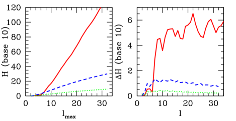
Figure 1: The information content as a function of the size of the fundamental domain and of $\ell_{\rm max}$: The left panel shows $H$ and right panel the increase per $\ell$, $\Delta H$, for (from the top downwards) T[2,2,2] (red solid line), T[4,4,4] (blue dashed line) and T[6,6,6] (green dotted line).

II.2 Measuring topology

While the previous subsection deals with a purely theoretical measure of detectability, namely the information content in a given map or matrix, we apply in this section two actual detection algorithms discussed in Ref. topo1 . For both we use likelihood, Eq. (1), or its logarithm $\chi^{2}$, Eq. (2). We exploit the fact that the the likelihood will be higher if observed map and template agree.

For the first analysis we compute the correlation between an observed map and a template and we search the global minimum of $\chi^{2}$ over all rotations of the $a_{\ell m}$ (corresponding to relative orientations of the observed map and template). In order to quantify possible false detections of the topological signal, we give an estimate of the null hypothesis, that is the possibility for an infinite universe to be taken for a universe with a non trivial topology. We use the following procedure: For each given topology (T[2,2,2], T[4,4,4], T[6,6,6]) we fix the template and generate several thousand random maps both from the chosen template and for an infinite universe. We then use the mean and standard deviation for both distributions to compute a signal to noise statistic,

$$S/N({\cal B},\chi^{2})=\frac{|\langle\chi^{2}\rangle_{\infty}-\langle\chi^{2}\rangle_{\cal B}|}{\sqrt{\sigma(\chi^{2})^{2}_{\infty}+\sigma(\chi^{2})^{2}_{\cal B}}}.$$ (14)

This corresponds to the distance between the means in units of the errors added in quadrature. We show results in Fig. 2, with the same colours/line styles as in Fig. 1. Again, we see that larger universes are more difficult to detect. The T[6,6,6] universe is barely detectable, while the others can be detect easily for $\ell_{\rm max}>16$.

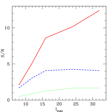
Figure 2: S/N for (from the top downwards) T[2,2,2] (red solid line), T[4,4,4] (blue dashed line) and T[6,6,6] (green dotted line).

The above test is somewhat ad-hoc, so that we compute additionally the probability that the $a_{\ell m}$ are actually drawn from the distribution described by the correlation matrix ${\cal B}$. This is often called the Bayesian evidence in astrophysical applications. Formally, the probability of a model (specified here via ${\cal B}$) is $p({\cal B}|a_{\ell m})$, which we can connect to the likelihood, Eq. (1) through Bayes theorem,

$$p({\cal B}|a_{\ell m})=p(a_{\ell m}|{\cal B})\frac{p({\cal B})}{p(a_{\ell m})}\propto{\cal L}({\cal B})p({\cal B}).$$ (15)

We will be interested in ratios of the these probabilities for different ${\cal B}$ (describing different topologies). As we have no a priori knowledge of the topology, we will take $p({\cal B})$ to be constant. However, the numerical value of ${\cal L}({\cal B})$ depends on the orientation of the template, so that we need to marginalise over the angles (see Ref. topo1 for more details, and inoue ; jaffe1 ; jaffe2 for other examples of the use of Bayesian evidence in topology). Unfortunately the likelihood is very strongly peaked in the vicinity of correct alignments. The numerical integration is difficult, even using adaptive schemes.

Having computed $p({\cal B}|a_{\ell m})$ we define a relative evidence for a topology as the ratio of this probability to the one for an infinite universe,

$$\Delta\log E({\cal B})=\log p({\cal B}|a_{\ell m})-\log p(1|a_{\ell m}).$$ (16)

This gives the relative probability that the $a_{\ell m}$ are due to a universe described by the topology and cosmology encoded in ${\cal B}$, compared to the probability that they are due to an infinite universe. Fig. 3 shows the strong dependence of the evidence on the size of fundamental domain, the figure looks somewhat similar to the one of $H$. One can further eliminate the dependence on the cosmological parameters by marginalising (integrating) over them as well. One of the motivations for this paper is to study the dependence of $\Delta\log E({\cal B})$ on the cosmological parameters and to understand which integrals are necessary. Finally, by also marginalising over a class of topologies (e.g. the X of cubic tori T[X,X,X]) and using the actually measured $a_{\ell m}$ we can compute the probability that our universe has that kind of topology.

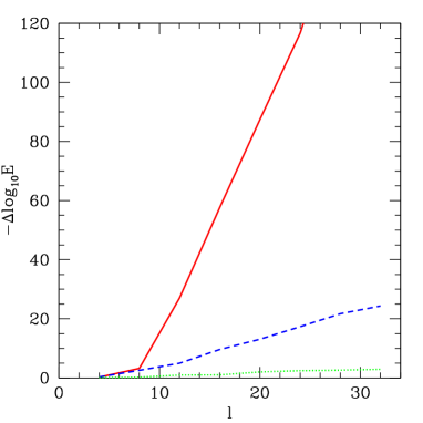
Figure 3: Evidence for (from the top downwards) T[2,2,2] (red solid line), T[4,4,4] (blue dashed line) and T[6,6,6] (green dotted line), compared to the $a_{\ell m}$ of an infinite universe.

III Physical effects at large scales

The shape of the universe leaves specific imprints on large scale CMB anisotropies at multipoles lower than $\ell\sim 60$ that can be detected via the correlation matrix of the $a_{\ell m}$ coefficients. Such scales suffer many problems. Firstly, it is at these scales that cosmic variance $\Delta C_{\ell}=\sqrt{2/(2\ell+1)}C_{\ell}$ is the largest. Then, at those scales several physical processes affect the CMB signal which may change our ability to detect non-trivial topologies and to measure their properties. In the following we will study the main effects, namely the reionisation and the integrated Sachs-Wolfe (ISW) effect, in addition to the relative size of the particle horizon as well as tensor modes and defects. In the next section, we will vary the relevant cosmological parameters and study their influence on the detection of the topological signal.

III.1 Relative size of fundamental domain and particle horizon

As discussed in the introduction, we fix the size of fundamental domain in units of $c/H_{0}$. Another key scale is the distance to the last scattering surface which is very close to the size of the particle horizon. In the following, we will not discriminate between these two. As light-rays move on geodesics with ${\rm d}s^{2}=0$ we can compute the particle horizon today in comoving coordinates from

$$\eta_{0}=\int_{0}^{t_{0}}\frac{c\;{\rm d}t}{a(t)}=c\int_{0}^{1}\frac{{\rm d}a}{a^{2}H(a)}.$$ (17)

The quantity relevant to us is the diameter of the particle horizon $D$ (the “size of the causal domain”), which, in units of $c/H_{0}$ is

$$D=\frac{2a_{0}H_{0}\eta_{0}}{c}=2\int_{0}^{1}{\rm d}x\left(\omega_{r}h^{-2}+\Omega_{m}x+\Omega_{\Lambda}x^{4}\right)^{-1/2},$$ (18)

where the new integration variable is the normalized scale factor $x\equiv a/a_{0}$, and we have assumed flat spacelike sections and dark energy in the form of a pure cosmological constant. The energy density in radiation $\omega_{r}\equiv\Omega_{r}h^{2}$ is fixed very precisely by the temperature of the CMB (assuming massless neutrini) to $4.2\times 10^{-5}$. Its presence changes the value of the above integral roughly by $\sqrt{\Omega_{r}}\approx 0.01$, i.e. the residual influence of the Hubble constant is of the order of $1\%$ only. Since we assume that the universe is flat, we have $\Omega_{m}=1-\Omega_{r}-\Omega_{\Lambda}$. In reality, the important scale is rather the distance to the last scattering surface (LSS), so that we should set the lower limit of integration to $x_{\rm LSS}\approx 1/1090$. This modifies the result by about 2% but does not change the conclusions.

The strength of the topological signal depends (among other things) on the ratio of the two scales. A universe that is much smaller than the causal domain leaves a strong imprint in the CMB, while one that is much larger will be impossible to distinguish from a truly infinite universe. The value of $D$ corresponds roughly to the largest $X$ that we can hope to detect. We show in Figures 1, 2 and 3 how the topology becomes easier to detect as the fundamental domain becomes smaller (for a fixed size of the particle horizon).

For a fixed size of the fundamental domain, the parameter affecting the ratio of the two scales is $\Omega_{\Lambda}$ as it changes $D$, see Fig. 4. If the matter density is very large, $\Omega_{m}\approx 1$, then the size of causal domain corresponds roughly to the size of a T[4,4,4] universe (in a purely matter-dominated universe, the horizon size equals twice the Hubble radius, hence $D=4$). On the other hand, the causal domain of a flat low-density universe can have an over 1000 times larger volume.

Figure 4: Diameter of the particle horizon, $D=2a_{0}\eta_{0}H_{0}/c$, for a flat universe and as a function of $\Omega_{\Lambda}$. This corresponds roughly to the maximal fundamental domain size $X$ that we can hope to detect.

The importance of the correct orientation of the fundamental domain was already discussed in Ref. topo1 . We found that the orientation is one of the critical parameters and needs to be taken into account in any analysis. This can be done by averaging quantities over the orientation (as is done for a Bayesian study), or by taking the maximum over all orientations (with the matched filter, or also when looking for correlated circles).

III.2 ISW effect

The CMB photons are influenced by the change in the gravitational potential through which they must pass. The effects arising from time-variable metric perturbations are generally known as the integrated Sachs-Wolfe effect sacwol in the linear regime and go by the names of Rees-Sciama effect rees86 and the effect from moving halos aghanim98 in the non-linear regime. The ISW effect depends on the time derivative of the gravitational potential. The anisotropies due to the ISW effect thus depend on the parameters of the background cosmology and are also tightly coupled to the clustering and the spatial and temporal evolution of the intervening structures. The most important contribution for topological studies is the late ISW effect due to the decay of the gravitational potential KoSt85 ; KaSp94 . This happens in a low matter density universe at the onset of dark energy (or spatial curvature) domination, when the increased rate of expansion of the universe reduces the amplitude of gravitational potential.

The power spectrum of the ISW can be written as a function of the power spectrum of the potential $P_{\Phi}(k)$ like

$$C_{\ell}=(4\pi)^{2}\ \int P_{\Phi}(k)k^{2}\;{\rm d}k\left[\int_{\eta_{\rm LSS}}^{\eta_{0}}2\dot{F}(\eta)j_{\ell}(kr)\;{\rm d}\eta\right]^{2}\,,$$ (19)

where the ${\rm LSS}$ subscript stands for the epoch of last scattering, $j_{\ell}(x)$ is the spherical Bessel function and $r$ is the comoving distance. $F(k,\eta)=D/x$ is the growth rate of the potential, where $x$ is the (normalized) scale factor and $D$ is the linear growth factor. The potential is related to the matter density contrast $\delta$ via the Poisson equation, $k^{2}\Phi=-\frac{3}{2}a_{0}^{2}\Omega_{m}H_{0}^{2}\delta/x$. In the matter-dominated era, the density contrast grows as $x$ and therefore the gravitational potential is constant. This is no longer the case in the dark-energy dominated era.

The ISW effect is seen mainly in the lowest $\ell$-values of the power spectrum where the cosmic variance is large. This makes its direct measurement very difficult. Since the time evolution of the potential that gives rise to the ISW effect may also be probed by observations of the large scale structure, one expects the ISW to be correlated with tracers of the large scale structure (see, e.g. Ref. CrTu96 ). This could conceivably help to remove it at least partially.

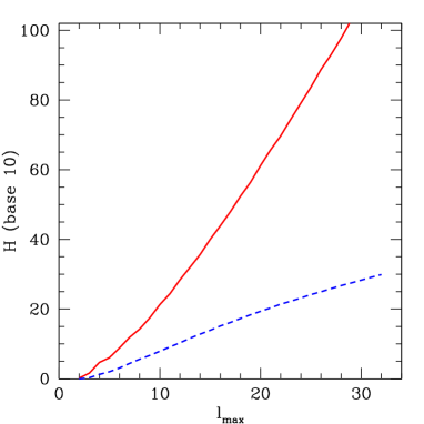
Figure 5: Influence of the ISW effect on the information content: The dashed blue line shows the $H$ for the T[4,4,4] model while the red line shows the information content for the same model but without ISW effect. The difference is very important.

We show in Fig. 5 the information content $H$ of our standard T[4,4,4] model (dashed blue line) and compare it to a fictitious case where the ISW effect was turned off (red solid line; the anisotropies are then only generated at last scattering). The ISW is clearly a very strong effect that needs to be taken into account correctly. We also checked its influence on the detection algorithms discussed in section II.2 and found the same result.

III.3 Reionisation

At reionisation, CMB photons scatter off free electrons, altering the CMB temperature anisotropies and inducing a polarised signal. The relevant effects in the case of topological studies are mostly those induced by reionisation on the CMB temperature anisotropies. At reionisation, the photon-electron interactions randomise the directions of propagation of the fraction of rescattered photons. As a result, the primary CMB anisotropies are suppressed and the power in the acoustic peaks is damped by a factor $\exp{(-2\tau)}$, where $\tau$ is the Thomson optical depth. Scales approaching the horizon at reionisation are barely affected by the scattering, the suppression is essentially efficient at small scales.

We investigate the effect of reionisation on the detectability of a non-trivial topology in Fig. 6 by comparing a universe with no reionisation (red solid line) and a universe with an optical depth compatible with the WMAP1 constraints ($\tau=0.166$, blue dashed line). The induced changes are negligible. The latest WMAP results suggest a significantly lower optical depth, therefore, the effect of reionisation is even smaller.

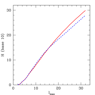
Figure 6: Influence of reionisation on the information content: The dashed blue line shows the $H$ for the T[4,4,4] model while the red line shows the information content for the same model but without reionisation. The difference is negligible.

III.4 Tensor modes and defects

Both gravitational waves and defects induce perturbations not primarily at decoupling, but throughout the whole evolution of the universe. Much of their contribution to the temperature anisotropies is therefore due to their late-time behaviour. In this they behave similarly to the integrated Sachs-Wolfe effect, and their contribution to the $a_{\ell m}$ will be mostly uncorrelated with the topological signal.

In a topologically non-trivial universe defects can stretch across the full fundamental domain (if they are at least one-dimensional). This may lead to a preferential alignment in certain directions. It also means that they cannot be larger than the size of the fundamental domain, so that their scaling behaviour has a cut-off at that scale. When the universe becomes larger, the defects will generically disappear (up to a possible net winding charge), leading to less fluctuation power on large scales.

Analyses wmap3_spergel ; us have restricted the contributions of primordial tensor modes and defects to be subdominant, and future measurements will improve limits substantially. We will consider them as a negligible source of “noise” for measurements of the topology. If ever their presence is detected, we should take them into account explicitely.

IV Sensitivity to cosmological parameters

We choose a fiducial model motivated by the WMAP3+SNLS results for a flat $\Lambda$CDM model wmap3_spergel , with $H_{0}=72.4\;{\mathrm{km}}\;{\mathrm{s}^{-1}}\;{\mathrm{Mpc}^{-1}}$, $n_{\rm S}=0.95$, $\Omega_{\Lambda}=0.75$, $\Omega_{b}h^{2}=0.0234$, and $\tau=0.085$. We then focus on the most relevant cosmological parameters and we explore their effects on the detection of the topological signal by varying in turn $H_{0}$, $n_{\rm S}$ and $\Omega_{\Lambda}$ (keeping all other parameters fixed). Table 1 shows the range of variation, corresponding to roughly the two-sigma limits of WMAP3 (with the exception of $\Omega_{\Lambda}$ where we also investigate other values). We do not expect the normalisation $A_{\rm S}$ or the baryon density $\Omega_{b}h^{2}$ to play an important role. In section III.3 we further saw that there is only a small difference between $\tau=0$ and the fiducial case. We conclude that variations of $\tau$ are also uncritical for measuring topology.

We limit ourselves to showing the results for the T[4,4,4] case since it is more realistic than T[2,2,2] while still giving a clear signal (as opposed to T[6,6,6]). The basic effects due to the parameter uncertainties do not depend on the size of the fundamental domain.

$h=$	$\{0.678,0.724,0.770\}$
$n_{\rm S}=$	$\{0.916,0.95.0,0.982\}$
$\Omega_{\Lambda}=$	$\{0.50,0.70,0.75,0.80,0.90\}$

Table 1: Parameter values investigated.

We show in the top panel of Fig. 7 how the information content $H$ depends on the three values of $n_{\rm S}$ (cf table 1). The other two panels show how such a variation of $n_{\rm S}$ affects the detection of a T[4,4,4] topology based on our fiducial model. To this end we simulated maps with the different values of $n_{\rm S}$ (and all other parameters fixed to the fiducial value) and then tested them against our fiducial model, applying the algorithms of section II.2. We find that the information content does not vary significantly. Also the detections measured by S/N (middle panel) and the Bayesian evidence (bottom panel) do not change for $\ell_{\rm max}<10$ with only small changes at higher resolutions (within the statistical fluctuations induced by the map realisations). We conclude that $n_{\rm S}$ can safely be fixed to the central value in table 1.

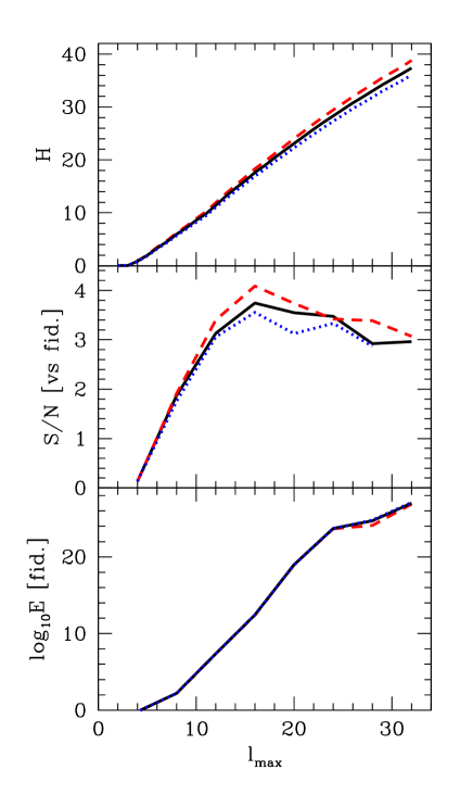
Figure 7: For T[4,4,4], the effect of varying $n_{\rm S}$: The top panel shows the information content, for the fiducial model (solid black line, $n_{\rm S}=0.950$) as well as $n_{\rm S}=0.916$ (dashed red line) and $n_{\rm S}=0.982$ (dotted blue line). The middle panel (S/N) and bottom panel (evidence) show how the detection changes when testing simulated maps against the fiducial model. The black solid line uses a map derived from the fiducial model, while the red dashed and blue dotted lines are for the smaller and larger $n_{\rm S}$ respectively.

The reduced Hubble parameter $h$ intervenes both in the size of the particle horizon (section III.1) and in the ISW effect (section III.2). We therefore expect some dependence on its value. Repeating the same analyses as for $n_{\rm S}$. We find that the results depend even less on $h$ than on $n_{\rm S}$, see Fig. 8. Clearly, $h$ can also be fixed to the central value in table 1.

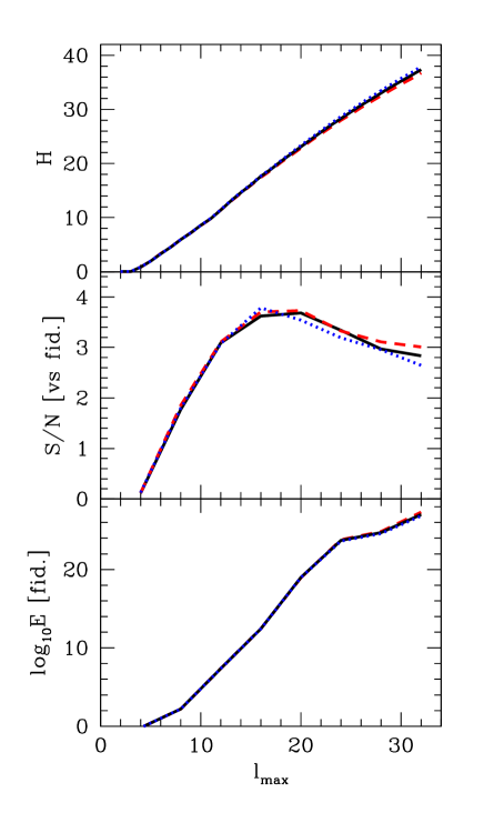
Figure 8: The effect of varying $h$ for T[4,4,4]: The top panel shows the information content, for the fiducial model (solid black line, $h=0.724$) as well as $h=0.678$ (dashed red line) and $h=0.770$ (dotted blue line). The middle panel (S/N) and bottom panel (evidence) show how the detection changes when testing simulated maps against the fiducial model. The black solid line uses a map derived from the fiducial model, while the red dashed and blue dotted lines are for the smaller and larger $h$ respectively.

We follow the same procedure as above, varying $\Omega_{\Lambda}$ only, for the values given in table 1. In the top panel of Fig. 9 we plot the information content for these models, with the largest $\Omega_{\Lambda}$ leading to the highest $H$. The larger $\Omega_{\Lambda}$, the larger the causal domain, but also the bigger the ISW contribution. The graph suggests that the effect due to the size of the fundamental domain dominates over the increase in “ISW noise”. As before, we then investigate how the detection changes if map and template have a different $\Omega_{\Lambda}$. In contrast to the two previous parameters, we find that there is a strong variation in the detectability. We only have a high S/N if map and template agree (black solid line in the middle panel). The maps with the next higher (red dashed line) and lower (blue dotted line) values of $\Omega_{\Lambda}$ are already below a significant detection limit, and the other cases lie even lower. The evidence shows the same behaviour, with the fiducial template leading to a much higher model probability than the others.

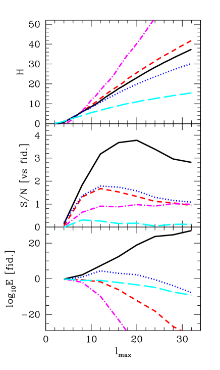
Figure 9: The effect of varying $\Omega_{\Lambda}$ for T[4,4,4]: The top panel shows the information content, for the fiducial model (solid black line, $\Omega_{\Lambda}=0.75$) as well as $\Omega_{\Lambda}=0.80$ (dashed red line), $\Omega_{\Lambda}=0.90$ (dot-dashed magenta line), $\Omega_{\Lambda}=0.7$ (dotted blue line), and $\Omega_{\Lambda}=0.50$ (long-dashed cyan line). The middle panel (S/N) and bottom panel (evidence) show how the detection changes when testing simulated maps against the fiducial model. The black solid line uses a map derived from the fiducial model. The line styles of the other models are the same as those of the information content (top panel).

A full analysis requires to explore all acceptable values of the cosmological parameters. Given that the topological signal remains nearly constant for all parameters except $\Omega_{\Lambda}$, it suffices to vary only $\Omega_{\Lambda}$ within the $2\sigma$ region allowed by WMAP3+SNLS.

V Conclusions

We have studied cubic torus universes, investigating the change of the topological signal with respect to the following effects: ISW, reionisation, size of causal horizon $D$, topological defects and primordial gravitational waves. We consider these to be the potentially most relevant effects for studying topology. We find that reionisation has negligible effect. The ratio $D$ to the size of the fundamental domain is the key quantity which limits our ability to detect a given topology. The ISW effect in turn is not correlated with the topological signal and so acts as an additional noise. The same is true for topological defects, and tensor modes, but they are experimentally constrained to a lower amplitude than the ISW effect. We conclude that only the ISW effect and the size of the causal horizon have to be considered.

An additional important parameter is the relative orientation of the fundamental domain topo1 . The methods we use take this already into account so that we do not discuss it in detail.

When searching for traces of a non-trivial topology, we have to test a priori templates for all cosmological models, varying the full set of cosmological parameters. We have shown here that, given the constraints from WMAP3+SNLS, only the allowed variation of $\Omega_{\Lambda}$ is able to affect significantly the detections. This parameter alters both the magnitude of the ISW effect and the size of the causal horizon. We find that the latter effect is more important and templates for several values of $\Omega_{\Lambda}$ are required for a complete analysis.

- (1) M. Lachièze-Rey and J.-P. Luminet, Phys. Rep. 254, 135 (1995).
- (2) J. Levin, Phys. Rep. 365, 251 (2002).
- (3) N. J. Cornish et al., Phys. Rev. Lett. 92, 201302 (2004).
- (4) B. Roukema et al., Astron. Astrophys. 423, 821 (2004).
- (5) J.-P. Luminet, Physics World 18, 22 (2005).
- (6) N. J. Cornish, D. Spergel and G. Starkmann, Class. Quantum Grav. 15, 2657 (1998).
- (7) J. G. Cresswell et al., Phys. Rev. D73, 1302 (2006).
- (8) A. Riazuelo et al., astro-ph/0601433 (2006).
- (9) M. Kunz et al., Phys. Rev. D73, 023511 (2006).
- (10) A. Riazuelo et al., Phys. Rev. D69, 103514 (2004).
- (11) A. Riazuelo et al., Phys. Rev. D69, 103518 (2004).
- (12) K. T. Inoue and N. Sugiyama, Phys. Rev. D67, 043003 (2003).
- (13) A. Niarchou, A. Jaffe, astro-ph/0602214 (2006).
- (14) A. Niarchou, A. Jaffe, astro-ph/0702436 (2007).
- (15) R. K. Sachs and A. M. Wolfe, Astrophys. J. 147, 73 (1967).
- (16) M.J. Rees and D. W. Sciama, Nature, 511, 611 (1986).
- (17) N. Aghanim et al., Astron. Astrophys. 334, 409 (1998).
- (18) L.A. Kofman and A.A. Starobinsky, Soviet Astr. Lett. 11, 271 (1985).
- (19) M. Kamionkowski and D.N. Spergel, Astrophys. J. 432, 7 (1994).
- (20) R.G. Crittenden and N. Turok, Phys. Rev. Lett. 76, 575 (1996).
- (21) D. N. Spergel et al., astro-ph/0603449 (2006).
- (22) N. Bevis et al., astro-ph/0702223 (2007)
- (23) K. M. Górski, É. Hivon and B. D. Wandelt, astro-ph/9812350 (1998); http://www.eso.org/science/healpix/ .