The contact process in disordered and periodic binary two-dimensional lattices

Abstract

The critical behavior of the contact process in disordered and periodic binary $2d$-lattices is investigated numerically by means of Monte Carlo simulations as well as via an analytical approximation and standard mean field theory. Phase-separation lines calculated numerically are found to agree well with analytical predictions around the homogeneous point. For the disordered case, values of static scaling exponents obtained via quasi-stationary simulations are found to change with disorder strength. In particular, the finite-size scaling exponent of the density of infected sites approaches a value consistent with the existence of an infinite-randomness fixed point as conjectured before for the $2d$ disordered CP. At the same time, both dynamical and static scaling exponents are found to coincide with the values established for the homogeneous case thus confirming that the contact process in a heterogeneous environment belongs to the directed percolation universality class.

I Introduction

The contact process (CP) Harris (1974), is a prototype model for the spatial spread of epidemics in biological systems. It describes epidemics in populations where each member can be in one of two states: infected (I) or susceptible (S) (so-called SIS models). The CP exhibits a non-equilibrium phase transition between an active and a non-active regime of the disease, behaving at its critical point according to the directed percolation (DP) universality class. This has been established by a range of analytical and numerical techniques Liggett (1985); Marro and Dickman (1999); Hinrichsen (2000); G.Ódor (2004) such as renormalization group analysis Hooyberghs et al. (2003); G.Ódor (2004), series expansions Jensen and Dickman (1993), Monte Carlo (MC) simulations Grassberger and De La Torre (1979); Grassberger (1989) and spectral analysis of the Liouville operator de Mendonça (1999); de Oliveira (2006). These analyses have been undertaken for simple topologies, mostly for homogeneous hyper-cubic lattices.

Recently, interest has turned towards the behavior of this process in disordered environments and revealed very peculiar features such as changing exponents and significantly different dynamics like Griffiths phases and activated scaling Moreira and Dickman (1996); Dickman and Moreira (1998); Vojta and Dickison (2005). In general, heterogeneous environments are typical in realistic systems, especially in the context of control of epidemics Finckha et al. (1999); Zhu et al. (2000); Otten et al. (2005); Forster and Gilligan (2007). Therefore, it is instructive to investigate the critical behavior of the CP under these conditions and in particular to establish the phase diagrams for such systems. In the past, the disordered CP (DCP) has been investigated in both one and two dimensions in a range of settings and revealed a continuous change in static critical exponents starting from the clean DP values Dickman and Moreira (1998); Hooyberghs et al. (2004); Neugebauer et al. (2006). In the $1d$ case, a strong-disorder renormalization group study allowed deep insight into the disordered process and revealed a dominating infinite-randomness fixed point (IRFP) for sufficiently strong disorder Hooyberghs et al. (2003). In the weak- to intermediate-disorder regime however, MC simulations and density-matrix renormalization group (DMRG) techniques Hooyberghs et al. (2004) as well as series expansions Neugebauer et al. (2006) found continuously varying disorder-dependent critical exponents which were found to approach those characteristic of an IRFP with increasing strength of disorder. For the $2d$ CP with site dilution, MC simulations showed a similar behavior, a continuous change in exponents with increasing disorder Moreira and Dickman (1996); Dickman and Moreira (1998) and, in retrospect Hooyberghs et al. (2004), giving evidence for the existence of an IRFP also in this case.

In this paper, we consider the phase diagram of the CP in a binary $2d$ lattice of sites with different recovery rates $\epsilon_{A}$ and $\epsilon_{B}$ drawn from a bimodal probability distribution. Extensive Monte Carlo (MC) simulations following Moreira and Dickman (1996) are employed in order to locate the line of critical points in the space of recovery rates $(\epsilon_{A},\epsilon_{B}$). As such simulations of disordered systems are numerically intensive due to very long relaxation times, analytical approximations are vital to constrain the region of phase space which contains the line of critical points. Here, we analyze the results obtained from the mean field approximation and further propose an approximate expression for critical points guided by the structure of the Liouville operator which governs the time evolution of the CP.

Also, the quasi-stationary (QS) simulation method de Oliveira and Dickman (2005a) is employed to investigate the static scaling behavior of the CP in this disordered system and to calculate the corresponding critical exponents. In particular, we study whether the process in this setting exhibits disorder-dependent changing exponents which cross over to values characteristic of an IRFP for sufficiently strong disorder as observed previously Hooyberghs et al. (2004); Dickman and Moreira (1998).

Following on, we investigate the behavior of the CP in a range of heterogeneous periodic lattices with different unit cells via MC simulations and test the validity of our analytical expression as well as standard mean field theory. The two analytical approaches, mean field and our alternative approximation, enable us to largely constrain the location of the critical points in both the disordered and the heterogeneous periodic lattices. Critical exponents are found to change continuously in the former case with increasing disorder and appear to approach the predicted values characteristic of an IRFP while they remain constant at their DP values in the latter.

The CP, its critical behavior and some of the theoretical foundations employed for its description are introduced in Sec. II. Our analysis of the disordered system is presented in Sec. III. In Sec. IV we investigate the CP in a range of heterogeneous periodic lattices in a similar fashion. Lastly, our findings are discussed in Sec. V and we summarize in Sec. VI.

II Background

In this section, we define the CP and give an overview of its critical behavior and the master-equation description by means of the Liouville operator. The CP is a non-equilibrium stochastic process in which an infection spreads via nearest-neighbor contact from site $i$ to $j$ at a transmission rate $w_{i\to j}$. Recovery of site $i$ is spontaneous and happens at a recovery rate $\epsilon_{i}$. In the thermodynamic limit, the ratio of these two rates is the control parameter of a second-order phase transition between a non-active phase where no infected sites remain as $t\to\infty$ and an active phase where the density of infected sites (order parameter) is non-zero as $t\to\infty$ Liggett (1985); Hinrichsen (2000); Marro and Dickman (1999).

For the CP in a system of size $N$ with sites $i=1\ldots N$ we denote the two possible states of site $i$ as $s_{i}=1$ (infected) or $s_{i}=0$ (susceptible). A microstate of the system, i.e. a snapshot of the infection states of all sites, can be defined as a vector $\mathbf{S}=(s_{1},\ldots,s_{N})^{T}$ and the probability of finding the system in a specific microstate at time $t$ is denoted by $P(\mathbf{S},t)$. Assuming the transition rates between microstates $\mathbf{S}$ and $\mathbf{S}^{\prime}$ to be $r_{\mathbf{S}\rightarrow\mathbf{S}^{\prime}}$, the time evolution of this probability follows the master equation which expresses the conservation of probability flow,

$$\partial_{t}P(\mathbf{S},t)=\sum_{\mathbf{S}^{\prime}}\left(r_{\mathbf{S}^{\prime}\rightarrow\mathbf{S}}P(\mathbf{S}^{\prime},t)-r_{\mathbf{S}\rightarrow\mathbf{S}^{\prime}}P(\mathbf{S},t)\right)~{},$$ (1)

where the transition rates $r_{\mathbf{S}\rightarrow\mathbf{S}^{\prime}}$ follow from the rules of the CP. The master equation can be recast in compact form by introduction of the Liouville operator $\hat{\mathcal{L}}$ which acts on the probability state vector $|P(t)\rangle$,

$$\partial_{t}\mbox{$|P(t)\rangle$}=\hat{\mathcal{L}}\mbox{$|P(t)\rangle$}~{},$$ (2)

the components of which are the probabilities of finding a system of $N$ sites in different states $|\sigma\rangle$ at time $t$, $\mbox{$|P(t)\rangle$}=\sum_{\sigma}\mbox{$\langle\sigma|P(t)\rangle$}\mbox{$|\sigma\rangle$}$. Here, $\left\{\mbox{$|\sigma\rangle$}\right\}$ is the orthonormal basis diagonal in the occupation number representation Marro and Dickman (1999); de Mendonça (1999). The precise form of $\hat{L}$ is most readily expressed in terms of hard-core bosonic creation and annihilation operators acting on site $i$, $a_{i}^{\dagger}$ and $a_{i}$, respectively,

$$\hat{L}=\sum_{i}\left(\epsilon_{i}(1-a^{\dagger}_{i})a_{i}+(1-a_{i})a^{\dagger}_{i}\sum_{j\in NN(i)}w_{j\to i}~{}a_{j}^{\dagger}a_{j}\right)~{},$$ (3)

where the first part destroys particles while the second part creates offspring Marro and Dickman (1999). The Liouville operator is non-Hermitian with matrix elements $\hat{\mathcal{L}}_{\sigma^{\prime}\sigma}\equiv\langle\sigma^{\prime}|\hat{\mathcal{L}}|\sigma\rangle$, which coincide with the transition rates from state $\sigma$ to state $\sigma^{\prime}\neq\sigma$ and $\hat{\mathcal{L}}_{\sigma\sigma}=-\sum_{\sigma^{\prime}\neq\sigma}\hat{\mathcal{L}}_{\sigma^{\prime}\sigma}$.

In principle, Eq. (2) can be solved by performing direct diagonalization of the $2^{N}\times 2^{N}$ real sparse (for lattice topologies) non-symmetric Liouville matrix. Its formal solution can then be expressed as

$$|P(t)\rangle = \sum_{i}\textrm{e}^{\lambda_{i}t}\mbox{$\langle e_{i}|P(0)\rangle$}~{}\mbox{$|e_{i}\rangle$}~{},$$ (4)

where $\lambda_{i}$ are the eigenvalues of the Liouville matrix with a complete set of eigenstates $|e_{i}\rangle$. The trivial solution $|e_{0}\rangle$ of the eigenproblem for the Liouville operator with $\lambda_{0}=0$ corresponds to the absorbing state of the system. All other eigenvectors $|e_{i}\rangle$ in finite systems have eigenvalues with negative real parts and thus decay exponentially with time. In the thermodynamic limit ($N\to\infty$), there is one eigenstate $|e_{1}\rangle$ with corresponding eigenvalue, $\lambda_{1}$, which is zero in the active and non-zero in the non-active phase. In a finite system, the value of $\lambda_{1}$ in the active (non-active) regime approaches a zero (non-zero) value with increasing $N$, thereby signaling the phase transition. The exact location of the transition can be extrapolated using finite-size data for moderate system sizes (e.g. $N\leq 16$) from direct diagonalization or density-matrix renormalization group calculations Hooyberghs et al. (2003); de Mendonça (1999).

III Disordered System

In what follows, we investigate the behavior of the CP on a lattice of two types of site, $A$ and $B$, characterized by different recovery rates $\epsilon_{A}$ and $\epsilon_{B}$, respectively. The recovery rate at site $i$, $\epsilon_{i}$, is drawn from the bimodal distribution

$$p(\epsilon_{i})=x~{}\delta(\epsilon_{i}-\epsilon_{A})+(1-x)~{}\delta(\epsilon_{i}-\epsilon_{B})~{},$$ (5)

where $x$ controls the relative concentration of $A$ and $B$ sites. The transmission rate, for simplicity, is the same for all possible links between nodes, $w_{i\to j}=w_{j\to i}=w$. As a further simplification, the timescale is set up by choosing $w=1/Z$ with $Z$ being the number of nearest-neighbor links per node ($Z=4$ for the topologies considered here).

III.1 MC Simulation

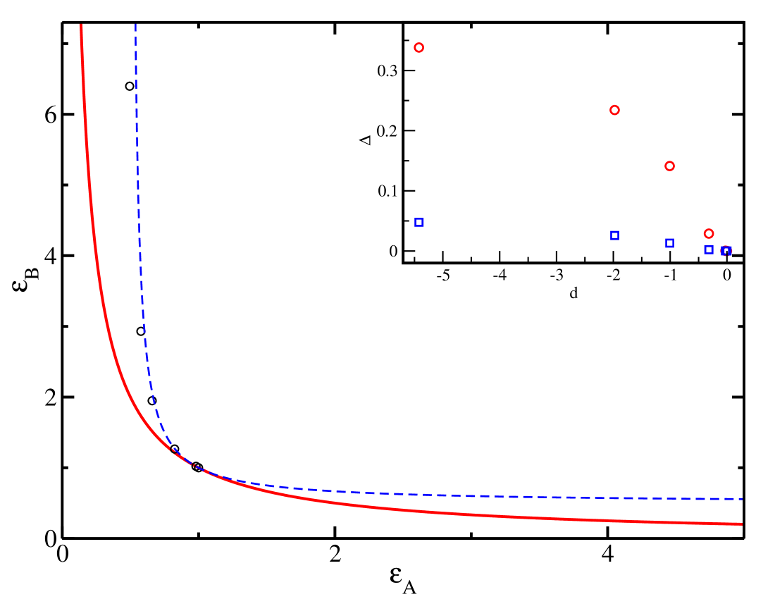
Figure 1: (Color online) The phase diagram for the CP on a disordered lattice with sites of recovery rates $\varepsilon_{A}$ or $\varepsilon_{B}$ drawn from the distribution Eq. (5) for the case $x=0.5$ obtained from MC simulation (dots), mean field (upper dashed line) and the analytical expression Eq. (8) (solid line). Inset shows the deviation $\Delta(d)$ as defined in the text for both mean field (blue $\Box$) and Eq. (8) (red $\circ$).

MC simulations are used to locate the critical point by starting from a single infection seed and averaging over $10^{6}$ realizations of the process each with a fresh realization of the disorder up to a maximum of $10^{6}$ time steps. We consider the case of $x=0.5$ and a range of values for $\epsilon_{A}$, aiming to find the corresponding critical $\epsilon_{B}$ for each. As previously observed Moreira and Dickman (1996), very slow dynamics are encountered, an effect that increases with disorder strength, i.e. the distance between $\epsilon_{A}$ and the homogeneous critical rate $\epsilon_{c}=0.60653(3)$ Marro and Dickman (1999). Following Moreira and Dickman (1996), the criterion of asymptotic monotonic growth or decay in order to assess whether the process is super- or sub-critical for a particular choice of rates is employed. For clarity of presentation, rescaled recovery rates $\varepsilon_{i}\equiv\epsilon_{i}/\epsilon_{c}$ are introduced in order for the homogeneous critical point to be conveniently located at $\varepsilon_{c}=\varepsilon_{A}=\varepsilon_{B}=1$. The resulting phase diagram, symmetric in $\varepsilon_{A}$ and $\varepsilon_{B}$, is shown in Fig. 1.

III.2 Mean Field Approximation

As outlined in the introduction, we are interested in analytically approximating the region where the phase separation line is located. To this end, we first present an approach based on mean field theory Marro and Dickman (1999). In this approximation, fluctuations and correlations are ignored rendering the master equation analytically tractable. For the case of the disordered system considered above, the governing equations for the mean concentrations of infected sites of type $A$ and $B$, $n_{A}$ and $n_{B}$ respectively, are given by

$$\frac{\partial n_{A}}{\partial t} = -\epsilon_{A}n_{A}+\frac{\epsilon_{*}}{2}(1-x)n_{B}(1-n_{A})+\frac{\epsilon_{*}}{2}xn_{A}(1-n_{A})$$

$$\frac{\partial n_{B}}{\partial t} = -\epsilon_{B}n_{B}+\frac{\epsilon_{*}}{2}xn_{A}(1-n_{B})+\frac{\epsilon_{*}}{2}(1-x)n_{B}(1-n_{B})~{},$$ (6)

where $\epsilon_{*}=wZ=1$ is the mean field critical value for the recovery rate in the homogeneous $2d$ square lattice. As usual for the mean field approximation in low-dimensional systems, $\epsilon_{*}$ significantly overestimates the true critical value for the homogeneous case, $\epsilon_{A}=\epsilon_{B}$. The locus of critical points in the parameter space ($\epsilon_{A},\epsilon_{B}$) separating non-active and active phases can be easily found from the solution of Eqs. (6) in the steady-state regime giving

$$\left\langle\frac{1}{\varepsilon_{i}}\right\rangle=1$$ (7)

with $\varepsilon_{i}=\epsilon_{i}/\epsilon_{*}$ where $\langle\dots\rangle$ denotes an average over disorder realizations.

The resulting phase separation line is shown in Fig. 1 along with the MC data presented above. Note that due to rescaling, mean field and numerical results coincide by construction at the homogeneous critical point. In order to allow a quantitative comparison between numerical results and approximation, a measure of difference between prediction and the true value obtained by MC simulation is needed. As such a measure, we consider the shortest distance $\Delta(d)$ between the prediction curve and an MC data point a (shortest path) distance $d$ away from the homogeneous point. This error quantity is suitable for quantitative analysis as it is a measure for the width of the region of uncertainty between the analytical prediction and the true critical line and will be symmetric about the homogeneous point for symmetric phase diagrams. The inset of Fig. 1 shows $\Delta(d)$ for the mean field approximation (blue squares).

As can be seen from the figure, the mean field approximation provides an upper bound to a region that contains the phase separation line. While the deviation $\Delta(d)$ is small in the vicinity of the homogeneous critical point ($\Delta<0.01$), it grows considerably as the degree of heterogeneity increases ($\Delta\approx 0.1$).

III.3 Alternative Analytical Approximation

Given that the mean field approximation appears to provide an upper bound to the region which contains the phase separation line, we are interested in obtaining an alternative analytical approximation that may provide a lower bound. In the following we will first present an approximate expression for the location of critical points in a heterogeneous system and then compare its predictions to the MC data of section III.1. Following on, we give a motivation for this approximation along with numerical support.

Statement and Comparison to Data

Consider a finite system of $N$ sites with arbitrary recovery rates $\epsilon_{i}$ ($i=1,\dots,N$). We will argue below that for such a system in the vicinity of the homogeneous critical point (all $\epsilon_{i}=\epsilon_{c}$) the expression

$$\prod_{j}^{N}\epsilon_{j}=\epsilon_{c}^{N}~{},$$ (8)

approximately predicts the location of critical points. For the disordered system presented earlier, this expression simplifies to $\epsilon_{c}^{2}=\epsilon_{A}~{}\epsilon_{B}$. Fig. 1 shows both the MC data presented earlier and the approximate line of critical points thus obtained. As can be seen from the figure, the alternative analytical approximation is found to provide a reliable lower bound to the region which contains the line of critical points. Hence, in combination with the mean field approximation discussed above, one can constrain this region. Considering the error $\Delta(d)$, it is found to show similar behavior to the one previously observed for the mean field data albeit an order of magnitude larger.

Motivation and Numerical Support

In the following we motivate Eq.(8) by considering the structure of the Liouville operator as defined in Sec. II. For the finite system introduced above, the eigenvalues of the Liouville operator, $\lambda$, are given by the characteristic equation,

$$\lambda^{-1}|\lambda\hat{I}-\hat{\mathcal{L}}|=Q_{N_{\text{max}}}(\{\epsilon_{i}\},\lambda)=\sum_{n=0}^{N_{\text{max}}}A_{n}(\{\epsilon_{i}\})\lambda^{n}=0~{},$$ (9)

where $Q_{N_{\text{max}}}(\lambda)$ is a polynomial in $\lambda$ of order $N_{\text{max}}$ ($N_{\text{max}}=2^{N}-1$) and division by $\lambda$ eliminates the trivial zero root for the absorbing state. It is our aim to solve this equation approximately in the vicinity of the homogeneous critical point where $\epsilon_{i}=\epsilon_{c}$.

To this end, we first consider the coefficients $A_{n}$ and look for features in their structure which may help in rendering the equation tractable. Generally, the $A_{n}$ can be expressed as

$$A_{n}(\{\epsilon_{i}\})=\sum_{m_{1},\ldots,m_{N}=0}\alpha^{(n)}_{m_{1},\ldots,m_{N}}~{}\prod_{j}^{N}\epsilon_{j}^{m_{j}}~{},$$ (10)

where the upper limits in the sum depend on $n$ but their precise values are not significant for the analysis below. We now assume that in the construction of the $A_{n}(\{\epsilon_{i}\})$ from the determinant of $\lambda\hat{I}-\hat{\mathcal{L}}$, the dominant contribution stems from terms with products of the same (or at least similar) powers of recovery rates at different sites. If this is true, the previous equation can be approximated as

$$A_{n}(\{\epsilon_{i}\})\simeq A_{n}\bigl{(}\prod_{j}^{N}\epsilon_{j}\bigr{)}=\sum_{m=0}^{m_{*}}\alpha_{m}^{(n)}~{}\left(\prod_{j}^{N}\epsilon_{j}\right)^{m}~{},$$ (11)

where $m_{*}\lesssim 2^{N}/N$. While this assumption may at first appear artificial, a justification can be found in the structure of the Liouville operator. The determinant of the Liouville matrix contains the sum of terms which are the products of the recovery rates (the transmission rates are chosen to be constant). A typical (representative) term contains a product of many recovery rates, each one picked from a different column. Assuming periodic boundary conditions, all sites in the system should enter the Liouville matrix in the same fashion. Therefore, in a typical term one would not expect to find an over-representation of a specific site leading to the statement that the (combinatorially) dominant terms correspond to products of recovery rates raised to powers that are close in value.

This argument only holds if one can be sure that the combinatorial weight of terms with homogeneous powers is not offset by the actual values of the recovery rates $\epsilon_{i}$. Otherwise, one could imagine the dominance of terms with very different powers of $\epsilon_{i}$ caused by the raising of values $>1$ to a high power. However, recall that for the clean CP at the homogeneous critical point, the true critical recovery rate is $<1$. Thus, close to this point, the critical recovery rates $\epsilon_{i}$ will always be close in value and $<1$ which means that the above argument about homogeneous powers is expected to hold in this regime. Further support will be given below in the form of numerical evidence using a specific system further down.

As explained in Sec.II, at criticality the highest non-trivial eigenvalue $\lambda_{1}(N)$ will be finite and tends to zero with increasing $N$. For the case of homogeneous recovery rates at criticality, $\epsilon_{i}=\epsilon_{c}$ and $Q_{N_{\text{max}}}(\{\epsilon_{c}\},\lambda_{1})=0$. Finally, by combination of this property and Eq. (11), we indeed find $\prod_{j}^{N}\epsilon_{j}=\epsilon_{c}^{N}$ for the homogeneous critical point which is precisely the statement presented above in Eq. (8).

The last step of our approximation then is to employ the same relation away from the homogeneous point and to use it to predict the locus of critical points.

More formally, the above condition for critical points can be derived from Eqs. (9) and (11) via a Taylor series expansion of $Q_{N_{\text{max}}}(\{\epsilon_{i}\},\lambda_{1})$ around the homogeneous critical point in $\ln(\epsilon_{i}/\epsilon_{c})$,

$$Q_{N_{\text{max}}}(\{\epsilon_{i}\},\lambda_{1})=\sum_{n=0}^{N_{\text{max}}}A_{n}(\{\epsilon_{i}\})\lambda_{1}^{n}$$ (12)

$$= \sum_{n=0}^{N_{\text{max}}}\left(\sum_{m=1}^{m_{*}}\alpha^{(n)}_{m}e^{m\sum_{i}^{N}\ln\epsilon_{i}}\right)\lambda_{1}^{n}$$

$$= \sum_{n=0}^{N_{\text{max}}}\sum_{m=1}^{m_{*}}\alpha^{(n)}_{m}\epsilon_{c}^{mN}\sum_{k=1}^{\infty}\frac{m^{k}}{k!}\ln^{k}\left(\prod_{i=1}^{N}\frac{\epsilon_{i}}{\epsilon_{c}}\right)\lambda_{1}^{n}=0~{}.$$

Here, we used the relation $Q_{N_{\text{max}}}(\{\epsilon_{c}\},\lambda_{1})=\sum_{n=0}^{N_{\text{max}}}A_{n}(\epsilon_{c}^{N})\lambda^{n}_{1}=0$ which leads to no constant term in the expansion and allows factorization of the above expression, i.e.

$$Q_{N_{\text{max}}}(\{\epsilon_{i}\},\lambda_{1})=S~{}\ln\left(\prod_{i=1}^{N}\frac{\epsilon_{i}}{\epsilon_{c}}\right)=0~{},$$ (13)

where

$$S=\sum_{n=0}^{N_{\text{max}}}\sum_{m=1}^{m_{*}}\alpha^{(n)}_{m}\epsilon_{c}^{mN}\sum_{k=1}^{\infty}\frac{m^{k}}{k!}\ln^{k-1}\left(\prod_{i=1}^{N}\frac{\epsilon_{i}}{\epsilon_{c}}\right)\lambda_{1}^{n}~{}.$$ (14)

Eq. (13) is obeyed if

$$\ln\left(\prod_{i=1}^{N}\frac{\epsilon_{i}}{\epsilon_{c}}\right)=0~{},$$ (15)

because $S\neq 0$ for arbitrary choice of $\epsilon_{i}$, which coincides with the condition given by Eq. (8). Alternatively, our approximate expression can be recast as an expectation value of logarithms Neugebauer et al. (2006),

$$E\left[\ln\frac{\epsilon}{\epsilon_{c}}\right]=0~{}.$$ (16)

Note that this procedure amounts to simply geometrically averaging the recovery rates and inserting them into the clean theory. Interestingly, the logarithm of rates well known from renormalization group analyses of the DCP and the random transverse-field Ising model G.Ódor (2004) arises naturally in our scheme.

In order to support the assumption about a dominant contribution to Eq. (10) from products of homogeneous powers of recovery rates, numerical evidence for a simple system is given below. Let us consider a $1d$ binary chain of sites $A$ and $B$ characterized by recovery rates $\epsilon_{A}$ and $\epsilon_{B}$, respectively, and spatially arranged as $\ldots ABAB\ldots$ with periodic boundary conditions. As a particular example, we analyze the coefficient $A_{0}(\epsilon_{A},\epsilon_{B})$ defined by Eq. (10), which reads (where $\alpha\equiv\alpha^{(0)}$)

$$A_{0} = \sum_{m_{A},m_{B}}\alpha_{m_{A}m_{B}}~{}\epsilon_{A}^{m_{A}}\epsilon_{B}^{m_{B}}$$ (17)

$$= \sum_{m=0}^{m_{*}}B_{m}(\epsilon_{A},\epsilon_{B})$$

with

$$B_{m}(\epsilon_{A},\epsilon_{B})=\left(\epsilon_{A}\epsilon_{B}\right)^{m}\times$$ (18)

$$\left(\alpha_{mm}+\sum_{j=1}^{m_{*}-m}\alpha_{m+j,m}\epsilon_{A}^{j}+\alpha_{m,m+j}\epsilon_{B}^{j}\right)~{},$$

which can be symbolically evaluated for relatively small systems ($N\leq 6$). Initially, $\epsilon_{A}$ and $\epsilon_{B}$ will both be set equal to $\epsilon_{c}$ consistent with our assumption that we investigate the vicinity of the homogeneous critical point. This enables us to investigate the relative magnitude of terms corresponding to different arrangements of powers. The terms $B_{m}$ effectively correspond to the contributions which contain either the homogeneous power $m$ or one recovery rate to the power $m$ along with the other recovery rate to a power greater than $m$. The magnitudes of the $B_{m}$ as functions of $m$ for the binary system of size $N=4$ and $N=6$ are shown in Fig. 2 (top panel). For both cases we observe sharp peaks centered at $m_{\text{max}}=3$ ($N=4$) and $m_{\text{max}}=12$ ($N=6$) indicating a dominant contribution from a narrow range of powers.

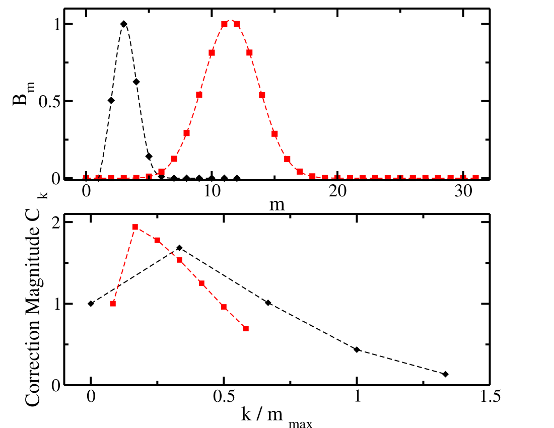
Figure 2: (Color online) Top panel: The terms $B_{m}$ as defined in Eq. (17) for a linear $AB$ chain of size $N=4$ (left black peak, $\Diamond$) and $N=6$ (right red peak, $\Box$) normalized by their maxima. Bottom panel: The correction terms $C_{k}$ as defined in Eq. (19) as a function of the relative difference between powers $k/m_{max}$ where $m_{max}$ is the location of the respective maximum in the upper panel. Symbols as before, all values have been normalized to the corresponding homogeneous contributions $C_{0}$.

The contribution to $A_{0}$ from purely homogeneous powers can be written as $C_{0}=\sum_{m=0}^{m_{*}}\alpha_{m,m}\left(\epsilon_{A}\epsilon_{B}\right)^{m}$ while corrections to this can be expressed as

$$C_{k}=\sum_{m=0}^{m_{*}-k}\left(\alpha_{m+k,m}~{}\epsilon_{A}^{m+k}\epsilon_{B}^{m}+\alpha_{m,m+k}~{}\epsilon_{A}^{m}\epsilon_{B}^{m+k}\right)$$ (19)

for $k>1$. The values of $C_{k}$ represent contributions from powers differing by $k$ from each other thus allowing a systematic investigation of the validity of our assumption. We are interested in the magnitude of these corrections as a function of the relative difference normalized by $m_{\text{max}}$ between powers in order to allow a comparison between different system sizes. While the homogeneous contributions $C_{0}$ are found not to be the most dominant, the corrections are peaked at $C_{1}$ for both systems considered and decay quickly with $k$. In particular, this decay happens increasingly rapidly with larger $N$ as a function of relative difference between powers, $k/m_{\text{max}}$ (cf. the red curve marked by squares ($\Box$) for $N=6$ and the black one marked by diamonds ($\Diamond$) for $N=4$ in Fig. 2) (bottom panel). A deviation of the values of $\epsilon_{A}$ and $\epsilon_{B}$ from their value of $\epsilon_{c}$ is found to reduce the dominance of the peaks presented above but does not immediately invalidate the assumption. However, when moving far away from the homogeneous critical point, the peaks flatten out indicating a breakdown of our approximation. In summary, all of the above findings can be considered to support the assumption about a dominant contribution of homogeneous powers of recovery rates in Eq. (17). We have undertaken a similar analysis for the coefficient $A_{1}$ and expect the same behavior for the remaining $A_{n}$. An analysis of $A_{n}$ (for $n\geq 2$) in a similar manner quickly becomes prohibitive due to the computational complexity of the resulting expressions. However, as $\lambda_{1}$ approaches zero with increasing $N$, these higher terms are expected to become increasingly irrelevant.

The question of whether one always expects to obtain a lower bound is addressed in the discussion (Sec. V) after more example cases have been compared to simulation data.

III.4 Critical Exponents from Quasi-Stationary Simulations

Investigations of the $2d$ DCP have been carried out in the past and have investigated both dynamic Moreira and Dickman (1996) and static scaling properties of the process Dickman and Moreira (1998). In general, the study of critical properties of the disordered process is complicated due to long relaxation times and ambiguity regarding the nature of scaling. In the following, we will investigate the static scaling of the disordered process by employing QS simulations de Oliveira and Dickman (2005a) and compare our results to both previous studies as well as theoretical predictions.

In the clean CP, the order parameter, $\lim_{t\to\infty}\rho$ is expected to obey the scaling form Marro and Dickman (1999)

$$\rho\sim L^{-x}~{}G\left(L^{1/\nu_{\perp}}(\epsilon-\epsilon_{c})\right)$$ (20)

where $x=\beta/\nu_{\perp}$, $L$ is the linear size of the system, and $\beta$ and $\nu_{\perp}$ are critical exponents. Further, $G$ is a scaling function which asymptotically behaves as $G(y)\to y^{\beta}$ as $y\to\infty$ and $G(y)\to\text{const.}$ for $y\to 0$. An analogous finite-size scaling form is expected to be obeyed by the order parameter fluctuations, $\chi=L^{d}\left(\overline{\rho^{2}}-\overline{\rho}^{2}\right)$, with the exponent $x$ replaced by $x^{\prime}=-\gamma/\nu_{\perp}$.

In order to apply the above scaling relations, one commonly considers QS values of observables as no true stationary state can exist in a finite system. The CP, when started from a fully infected system, initially relaxes while spatial correlations grow towards the system size and temporal correlations decay. Once the spatial correlation length becomes comparable to the size of the system, the process enters a QS regime characterized by a time-independent non-zero transition rate to the absorbing state. In this regime, the QS density $\overline{\rho}$, i.e. the density $\rho$ conditioned on survival, attains a constant value. In the past, analysis of this metastable state in computer simulations has proved to be notoriously difficult. Usually, the time-dependent density of infected sites conditioned on survival, $\overline{\rho}$, which becomes stationary in the QS regime, is investigated Marro and Dickman (1999). Problematically though, it is neither clear at what time this density has converged to its QS value nor when the QS state starts to decay due to finite-size effects Lübeck and Heger (2003). Therefore, a range of alternative approaches have been proposed which enable an observation of this metastable regime (see Ref. de Oliveira and Dickman (2005a) and references therein). Here, we employ the QS simulation method de Oliveira and Dickman (2005a) which allows a direct sampling of the QS state by eliminating the absorbing state and redistributing its probability mass over the active states.

Following Ref. de Oliveira and Dickman (2005a), one starts from the master equation Eq. (1). For the CP, this equation does not admit a non-trivial stationary solution for a finite system due to the existence of the absorbing state $\mathbf{0}$ which can be entered but not be left. The QS solution mentioned above can be defined as

$$\overline{P}(\mathbf{S})=\lim_{t\to\infty}\frac{P(\mathbf{S},t)}{P_{s}(t)}~{},$$ (21)

where $P_{s}(t)$ denotes the survival probability of the process at time $t$. Now, consider a modification of the governing equation,

$$\partial_{t}Q(\mathbf{S},t) = \sum_{\mathbf{S}^{\prime}}[r_{\mathbf{S}^{\prime}\rightarrow\mathbf{S}}Q(\mathbf{S}^{\prime},t)-r_{\mathbf{S}\rightarrow\mathbf{S}^{\prime}}Q(\mathbf{S},t)$$ (22)

$$+r_{\mathbf{S^{\prime}}\to\mathbf{0}}Q(\mathbf{S^{\prime}},t)Q(\mathbf{S},t)]~{}.$$

where $Q(\mathbf{S},t)$ denotes the probability of a new process governed by this equation being in state $\mathbf{S}$ at time $t$. The stationary solution of Eq. (22), $\overline{Q}(\mathbf{S})$, coincides with the QS probability of the original process as can be seen by substituting $Q(\mathbf{S},t)=P_{s}(t)\overline{P}(\mathbf{S})$ and noticing that in the QS regime $dP_{s}/dt=-P_{s}\sum_{\mathbf{S}}r_{\mathbf{S}\to\mathbf{0}}\overline{P}(\mathbf{S})$. In that case, the right-hand side of Eq. (22) is equal to zero if $\overline{Q}(\mathbf{S})=\overline{P}(\mathbf{S})$ as required. The last term in Eq. (22) can be viewed as a redistribution of probability from the absorbing state to the active states according to their probability de Oliveira and Dickman (2005a). Thus, if one could sample from a process governed by Eq. (22), it would converge to a true stationary state governed by the QS probability distribution of the original process. Such a process is given by the original CP where all transitions to the absorbing state are instead redirected to an active state randomly chosen according to its probability. As in practice this probability is not known a priori, an estimate is generated by sampling from the history of the process. Generally, the method has proved to be efficient with fast and reliable convergence after optimization of history sampling parameters de Oliveira and Dickman (2005a, b). The approach is particularly suited to a study of the DCP for which, in dynamic single-seed MC simulations employed for the DCP in the past Moreira and Dickman (1996); Vojta and Dickison (2005), the question of whether the asymptotic limit of the process had been reached was frequently contested. In contrast, QS simulations offer a clear means of ensuring this: a true stationary average whose convergence can be monitored.

Table 1: The critical rates $\epsilon_{B}$ for a given $\epsilon_{A}$, critical exponents $x$ and $x^{\prime}$ for the disordered systems discussed in the text.

$\epsilon_{A}$	$\epsilon_{B}$ (critical)	$x$	$x^{\prime}$
0.60653	0.60653(3)	0.795(4)	0.42(3)
0.595	0.6188(3)	0.796(5)	0.41(5)
0.5	0.7676(4)	0.83(1)	0.39(3)
0.4	1.1815(5)	0.92(4)	-
0.35	1.7775(5)	0.93(4)	-
0.3	3.89(1)	0.99(5)	-

Here, we have investigated the $2d$ DCP with bimodal disorder in its recovery rates drawn from the distribution Eq. (5) by means of QS simulations for up to $10^{8}$ time steps and systems of sizes $L=8,\dots,128$ sites averaging over no less than $10^{3}$ disorder realizations. At the critical point, fits to the above finite-size scaling relations yielded estimates for the exponents $x$ and $x^{\prime}$. For the homogeneous case, the well-established values for the exponents of the DP universality class are recovered ($\beta/\nu_{\perp}=0.795(7)$, $\gamma/\nu_{\perp}=0.41(2)$ Lübeck (2004)). As the degree of disorder, i.e. the difference between recovery rates $\epsilon_{A}$ and $\epsilon_{B}$, is increased, the measured exponents are found to change with disorder strength where $x$ increases while $x^{\prime}$ decreases (cf. Tab. 1). For strong heterogeneity, no credible fluctuation exponent could be extracted from the data due to strong sample-to-sample fluctuations. This is unfortunate as it prevents us from testing the validity of the hyperscaling relation $\frac{\gamma}{\nu_{\perp}}=d-\frac{2\beta}{\nu_{\perp}}$. A similar relation for dynamical exponents had previously Moreira and Dickman (1996) been found to break down for the DCP.

IV Heterogeneous Periodic Lattices

In order to investigate the range of validity of Eq. (8), we now turn to the behavior of the CP on lattices with periodic arrangements of sites of type $A$ and $B$ discussed above.

For such systems, the equation for the locus of critical points reads

$$\epsilon_{A}^{c_{A}}\epsilon_{B}^{c_{B}}=\epsilon_{c}~{},$$ (23)

where $c_{A}$ and $c_{B}$ denote the concentration of species $A$ and $B$, respectively. Three lattice systems have been analyzed with $c_{A}=c_{B}=1/2$: (i) a standard chessboard lattice [Fig. LABEL:f1], (ii) a big chessboard lattice [Fig. LABEL:f2] and (iii) a lattice of rows [Fig. LABEL:f3]. Extensive MC simulations ($3\times 10^{6}$ runs up to $t=3000$ maximum time steps) starting from a single infection seed were performed for these heterogeneous lattices. Unlike in the disordered case, for heterogeneous systems, asymptotic scaling relations that are well-known from the homogeneous case are found to hold. At criticality, the average number of infected sites $\langle N(t)\rangle$, the mean squared radius $\langle R^{2}\rangle$ of spread of the CP (where angular brackets denote averaging over all realizations and over active realizations at time $t$, respectively) and the survival probability $P(t)$ follow asymptotic scaling laws Marro and Dickman (1999),

$$\langle N\rangle\sim t^{\eta}~{},\quad\langle R^{2}\rangle\sim t^{2/z}~{},\quad P\sim t^{\delta}~{},$$ (24)

where $\eta$, $\delta$ and $z$ are the dynamical critical exponents characteristic of the universality class. These scaling relationships provide a method for finding the critical value of the control parameter by fitting the observables to the above scaling forms following Ref. Grassberger (1989). Furthermore, the dynamical critical exponents can be determined from the fit.

As expected, the numerical data agree very well with the analytical predictions given by Eq. (23) [cf. the circles with the solid line for $\varepsilon_{A}\simeq\varepsilon_{B}\simeq 1$ in Figs. LABEL:f1-LABEL:f3] in the neighborhood of the homogeneous critical point, and start to deviate from the predicted phase-separation line for $\varepsilon_{A,B}\gtrsim 1$ consistent with the validity of our approximation. The quality of the analytical approximation is high for the standard chessboard case ($\Delta<0.03$ for a very large range of rates) but becomes worse for the big chessboard ($\Delta$ up to $0.15$ when moving away far from the homogeneous point) and especially for rows in the range of large values of $\varepsilon_{A,B}\gg 1$.

Furthermore, we have studied two lattices with different concentrations of nodes A and B, i.e. $c_{A}/c_{B}=2/1$ – lattice (iv) [see Fig. LABEL:f4], and $c_{A}/c_{B}=3/1$ – lattice (v) [see Fig. LABEL:f5]. In these cases, the phase-separation lines are not symmetric about the bisector in the $\varepsilon_{A}-\varepsilon_{B}$ plane. As can be seen from Figs. LABEL:f4-LABEL:f5, the results of MC simulations of the CP on these lattices are again in good agreement with the analytical expression given by Eq. (23), especially near the homogeneous critical point (cf. the circles with the solid line for $\varepsilon_{A}\simeq\varepsilon_{B}\simeq 1$ in Figs. LABEL:f4-LABEL:f5). In case of lattice (iv), the error as shown in the inset indicates a similar order of magnitude degree of accuracy as in the simple chessboard case before ($\Delta<0.05$ for a large range of rates) while for lattice (v) the approximation is found to deteriorate [with approximately twice the value of $\Delta$ as compared to lattice (iv)].

It is instructive to compare the expression for the phase-separation line given by Eq. (23) with the results obtained from the master equation within the standard mean field approximation. Expressions similar to Eqs. (6) can be found for all the different lattices and solved for the critical rates in the steady-state regime. The resulting expressions for all the lattices are summarized in Table 2.

Table 2: The expressions for the phase-separation lines for the CP on different lattices (first column) obtained according to Eq. (23) (second column) and within the standard mean field approach (third column).

	lattice type	Eq. (23)	mean field
	(i)	$\varepsilon_{B}=1/\varepsilon_{A}$	$\varepsilon_{B}=1/\varepsilon_{A}$
	(ii)	$\varepsilon_{B}=1/\varepsilon_{A}$	$\varepsilon_{B}=\varepsilon_{A}/(2\varepsilon_{A}-1)$
	(iii)	$\varepsilon_{B}=1/\varepsilon_{A}$	$\varepsilon_{B}=\varepsilon_{A}/(2\varepsilon_{A}-1)$
	(iv)	$\varepsilon_{B}=1/\varepsilon_{A}^{2}$	$\varepsilon_{B}=1/(2\varepsilon_{A}-1)$
	(v)	$\varepsilon_{B}=1/\varepsilon_{A}^{3}$	$\varepsilon_{B}=\varepsilon_{A}/(2\varepsilon_{A}^{2}-1)$

As follows from Table 2, the mean field result coincides with the expression for the phase-separation line given by Eq. (23) for the standard chessboard configuration [lattice (i)] and gives a different prediction for all other cases studied. The rescaled mean field results agree very well with MC data around the homogeneous point but display deviations for $\varepsilon_{A,B}\gg 1$. Looking at the corresponding errors $\Delta(d)$, they are found to be of the same order as found for the previous analytical approximation.

The fact that for the simple chessboard lattice our earlier prediction and the mean field result coincide reveals this case to be special in that the rescaled mean field does not over- but underestimate the true critical values. In all other studied lattices, the rescaled mean field results for the phase-separation lines lie above the numerical data [cf. the dashed lines with the circles in Figs. LABEL:f2-LABEL:f5] and thus lead to an overestimate of the value if $\varepsilon_{B}$ for a given $\varepsilon_{A}$. This means that for these cases, mean field estimates of critical values can serve as an upper bound on the critical recovery rate. In contrast, the phase-separation lines predicted by Eq. (23) provide a consistent underestimate of the true critical line for all studied lattices and therefore a lower bound (cf. the solid lines in relation to the circles in Figs. LABEL:f2-LABEL:f5 and see the arguments given in Sec. V) for the critical thresholds.

In order to more systematically investigate how our alternative analytical approximation deteriorates as the spatial arrangement of sites becomes “less mixed”, we consider a lattice like the big chessboard, lattice (ii), but vary the linear size $L$ of the square contiguous regions of $A$ or $B$ sites. The resulting deviation $\Delta(d)$ as defined above at critical $\epsilon_{B}$ for a choice of $\epsilon_{A}=0.9$, i.e. appreciably far away from the homogeneous critical point, as a function of $L$ is shown in Fig. LABEL:fig:box_scaling. One can see that for $L\geq 4$ the accuracy quickly becomes worse than for any rate and lattice previously considered indicating a rapid breakdown of the approximation.

Finally, the universality of the critical behavior of the CP in binary lattices was investigated. The expected dynamical power-law scaling relations [see Eqs. (24)] were verified and used to obtain the resulting critical exponents for several sets of parameters $(\varepsilon_{A},\varepsilon_{B})$ on the phase-separation lines for all the lattices. The evaluation of the exponents was performed following Ref. Grassberger and De La Torre (1979) through extensive numerical simulations performing averages of $3\times 10^{6}-10^{7}$ runs to a maximum of $t=3000$ time steps. Our results obtained for the different lattices indicate that, within error bars, the exponents in all cases coincide with those established for $2d$ processes in the DP universality class ($\eta=0.2295(10)$, $\delta=0.4505(10)$,$2/z=1.1325(10)$) Voigt and Ziff (1997). Furthermore, the static scaling exponent ratios determined analogously to the disordered case from the QS simulation method are found to coincide with those of the DP universality class.

V Discussion

Looking back at the phase diagrams for both the disordered and the periodic systems, the introduction of disorder in the form of a random placement of $A$ and $B$ sites appears to enhance the activity of the system. In Fig. 1, MC data for the disordered system are presented and one notices a shallow initial increase in critical $\varepsilon_{B}$ for a given $\varepsilon_{A}$ as one moves away from the homogeneous critical point followed by an increasingly steep increase at values of $\varepsilon_{A}\lesssim 0.5$ ($\epsilon_{A}\lesssim 0.3$). Comparing this behavior with the corresponding periodic system [Fig. LABEL:f2], the critical value for $\varepsilon_{B}$ in the disordered system is found to be much larger.

Considering the arrangement of, say, $A$ sites as a site percolation problem, one notices that for concentrations below the percolation threshold ($x_{c}\simeq 0.59$) no infinite cluster of such sites can exist. Therefore, no matter how small (but non-zero) the corresponding recovery rate $\varepsilon_{A}$ is, it will require a finite value of $\varepsilon_{B}$ to render the system critical as a finite cluster cannot support an active state indefinitely. Conversely, above the percolation threshold there exists a finite value of $\varepsilon_{A}$ below which the system will be active irrespective of the value of $\varepsilon_{B}$. Therefore, for the case of $x=0.5$, no asymptote at any non-zero value of $\epsilon_{A}$ would be expected. Interestingly, the mean field expression Eq. (7) does predict an asymptote at $\epsilon_{A}=x$ albeit for any concentration of sites.

Turning to the CP in heterogeneous periodic lattices, for a range of cases the combination of the standard mean field approximation and our alternative analytical approximation is useful in practice to pinpoint the location of the transition a priori. Indeed, a tight fit for all cases (with the exception of the simple chessboard lattice) can be attested. In particular, the influence of spatial structure on the quality of our approximation becomes evident. The less mixed the arrangement of $A$ and $B$ sites becomes, the worse the fit of the approximation is found to be as indicated by the results in Fig. LABEL:fig:box_scaling. In order to evaluate the practical relevance of our approximation, the question of whether it is expected to always yield a lower bound has to be addressed. To this end, we define an average clustering coefficient specific to a particular lattice configuration and site type. For sites of type $A$ for instance, define $C_{A}=n_{\text{NN,A}}/Z$ where $n_{\text{NN,A}}$ denotes the number of nearest neighbors of site type $A$ (and analogously for $B$ sites). For the case of a periodic lattice with a $1:1$ mixture of $A$ and $B$ sites, consider the minimally-clustered configuration, that is the standard chessboard [lattice (i)], for which $C_{A}=C_{B}=0$. We know that for this case our approximation yields a very tight lower bound to the true curve of critical points. Any lattice with the same concentration of sites will necessarily have a higher clustering coefficient, i.e. a larger fraction of contiguous regions of $A$ and $B$ sites. Assuming different recovery rates for the two types of site, the disease will have the tendency to survive longer in a constellation $AABB$ as compared to $ABAB$ due to the adjacency of two sites of lower recovery rate (say $A$) which enhances the probability of infection and reinfection in the $AA$ arrangement. This activity-enhancing effect is not offset by the fact that two less reactive sites (say $B$) are also bordering as their faster (than A sites) recovery is largely independent of spatial arrangement. Indeed, a direct diagonalization of the corresponding Liouville operator for these two different arrangements of sites readily confirms this intuition. One obtains a lower (absolute) value for the real part of the first non-trivial eigenvalue in case of an arrangement $AABB$ as compared to $ABAB$ indicating a slower approach to the absorbing state in a finite system.

From this we conclude that for any periodic arrangement of $A$ and $B$ sites our alternative analytical approximation is expected to yield a lower bound to the phase separation line. Similarly, the arrangement used in lattice (iv) is the minimally-clustered ($C_{A}=1/2$, $C_{B}=0$) arrangement with a $1:2$ concentration of sites and is found to give a lower bound leading us to expect the same behavior for any arrangement of $A$ and $B$ sites in this ratio. Therefore, by testing the minimally-clustered case for the desired concentration one should in practice be able to verify whether or not a lower bound is expected by our approximation.

Considering the critical exponents obtained for both the disordered and the periodic systems, they are found to be disorder dependent in the former case while they remain at their DP values in the latter. Predictions from a numerical implementation of the strong-disorder renormalization scheme in $2d$ predict an exponent value $x_{\text{strong}}=1.0$ at an IRFP Hooyberghs et al. (2004); Motrunich et al. (2000). At the same time, as conjectured in Hooyberghs et al. (2004) and supported by numerical evidence, the DCP in $2d$ is likely to be dominated by such a fixed point for sufficiently strong disorder similar to the $1d$ case. Thus, one would expect disorder-dependent varying exponents which approach their values expected at an IRFP for strong disorder. Our results support this picture: we find continuously varying disorder-dependent exponents and a finite-size scaling exponent $x$ which is compatible with the predicted value at an IRFP for the strongest disorder under consideration ($\epsilon_{A}=0.3$).

Regarding the unchanged exponents in the case of periodic systems, these findings confirm theoretical arguments Vojta (2006) which make a prediction about the universal behavior of the CP in heterogeneous and disordered systems. Under coarse-graining the heterogeneity present in systems such as the heterogeneous periodic lattices considered in this paper will eventually become homogeneous after a finite number of iterations of the coarse-graining procedure. Thus, one would expect the critical behavior of the CP to be governed by the conventional clean fixed point of the renormalization group transformations G.Ódor (2004).

VI Conclusion

In conclusion, we have investigated the contact process in both heterogeneous disordered and periodic $2d$ systems (binary lattices). The phase diagram has been obtained via extensive Monte Carlo simulation. Furthermore, two approximations have been successfully used in order to constrain a region of phase space which contains the line of critical points. First, the mean field approximation was employed to give a phase separation line which provided an upper bound to this region in almost all systems. Second, an alternative analytical approximation based on the structure of the Liouville operator was motivated and used to obtain a respective lower bound in all cases. The quality of both approximations was quantitatively analyzed for all systems and found to be high in the vicinity of the homogeneous critical point but increasingly worse when moving to higher degrees of heterogeneity. In general, we conclude that the strategy of constraining a region deemed to contain the critical points a priori may be of practical interest particularly in connection with disordered systems in which long relaxation times render computer simulations very costly.

Lastly, critical exponents obtained for the disordered system are in good agreement with data from previous investigations obtained in the crossover region between the homogeneous case and strong disorder. In particular, the values obtained for the critical exponent $x$ are compatible with the existence of an IRFP in the $2d$ DCP for sufficiently strong disorder. At the same time, as expected the well-known DP exponents were recovered for all periodic systems.

References

- Harris (1974) T. Harris, Annals of Probability 2, 969 (1974).
- Liggett (1985) T. M. Liggett, Interacting Particle Systems (Springer-Verlag, New York, 1985).
- Marro and Dickman (1999) J. Marro and R. Dickman, Nonequilibrium Phase Transitions in Lattice Models (Cambridge University Press, Cambridge, 1999).
- Hinrichsen (2000) H. Hinrichsen, Adv. Phys. 49, 815 (2000).
- G.Ódor (2004) G.Ódor, Rev. Mod. Phys. 76, 663 (2004).
- Hooyberghs et al. (2003) J. Hooyberghs, F. Iglói, and C. Vanderzande, Phys. Rev. Lett. 90, 100601 (2003).
- Jensen and Dickman (1993) I. Jensen and R. Dickman, J. Stat. Phys. 71, 89 (1993).
- Grassberger and De La Torre (1979) P. Grassberger and A. De La Torre, Ann. Phys. (N.Y.) 122, 373 (1979).
- Grassberger (1989) P. Grassberger, J. Phys. A 22, 3673 (1989).
- de Mendonça (1999) J. R. G. de Mendonça, J. Phys. A: Math. Gen. 32, L467 (1999).
- de Oliveira (2006) M. J. de Oliveira, Phys. Rev. E 74, 41121 (2006).
- Moreira and Dickman (1996) A. G. Moreira and R. Dickman, Phys. Rev. E 54, R3090 (1996).
- Dickman and Moreira (1998) R. Dickman and A. G. Moreira, Phys. Rev. E 57, 1263 (1998).
- Vojta and Dickison (2005) T. Vojta and M. Dickison, Phys. Rev. E 72, 036126 (2005).
- Finckha et al. (1999) M. R. Finckha, E. S. Gacekb, H. J. Czemborc, and M. S. Wolfed, Plant Pathology 48, 807 (1999).
- Zhu et al. (2000) Y. Zhu, H. Chen, J. Fan, Y. Wang, Y. Li, J. Chen, J. Fan, S. Yang, L. Hu, H. Leungk, et al., Nature 406, 718 (2000).
- Otten et al. (2005) W. Otten, J. A. N. Filipe, and C. A. Gilligan, Ecology 86, 1948 (2005).
- Forster and Gilligan (2007) G. A. Forster and C. A. Gilligan, PNAS 104, 4984 (2007).
- Hooyberghs et al. (2004) J. Hooyberghs, F. Iglói, and C. Vanderzande, Phys. Rev. E 69, 66140 (2004).
- Neugebauer et al. (2006) C. J. Neugebauer, S. V. Fallert, and S. N. Taraskin, Phys. Rev. E 74, 040101(R) (2006).
- de Oliveira and Dickman (2005a) M. M. de Oliveira and R. Dickman, Phys. Rev. E 71, 016129 (2005a).
- Lübeck and Heger (2003) S. Lübeck and P. C. Heger, Phys. Rev. E 68, 056102 (2003).
- de Oliveira and Dickman (2005b) M. M. de Oliveira and R. Dickman, Braz. J. Phys. 36, 3A (2005b).
- Lübeck (2004) S. Lübeck, Int. J. Mod Phys B 18, 3977 (2004).
- Voigt and Ziff (1997) C. A. Voigt and R. M. Ziff, Phys. Rev. E 56, R6241 (1997).
- Motrunich et al. (2000) O. Motrunich, S.-C. Mau, D. A. Huse, and D. S. Fisher, Phys. Rev. B 61, 1160 (2000).
- Vojta (2006) T. Vojta, J. Phys. A 39, R143 (2006).