The building up of the disk galaxy M33
and the evolution of the metallicity gradient

Abstract

Context. The evolution of radial gradients of metallicity in disk galaxies and its relation with the disk formation are not well understood. Theoretical models of galactic chemical evolution make contrasting predictions about the time evolution of metallicity gradients.

Aims. To test chemical evolution models and trace the star formation and accretion history of low luminosity disk galaxies we focus on the Local Group galaxy M33.

Methods. We analyze O/H and S/H abundances in planetary nebulae, Hii regions, and young stars, together with known [Fe/H] abundances in the old stellar population of M33. With a theoretical model, we follow the time evolution of gas (diffuse and condensed in clouds), stars, and chemical abundances in the disk of M33, assuming that the galaxy is accreting gas from an external reservoir.

Results. Our model is able to reproduce the available observational constraints on the distribution of gas and stars in M33 and to predict the time evolution of several chemical abundances. In particular, we find that a model characterized by a continuous infall of gas on the disk, at a rate of $\dot{M}_{\rm inf}\approx 1$ $M_{\odot}$ yr^-1, almost constant with time, can also account for the relatively high rate of star formation and for the shallow chemical gradients.

Conclusions. Supported by a large sample of high resolution observations for this nearby galaxy, we conclude that the metallicity in the disk of M33 has increased with time at all radii, with a continuous flattening of the gradient over the last $\sim 8$ Gyr.

1 Introduction

Local Group (LG) galaxies, with their variety of morphological types, are ideal candidates for testing the predictions of galactic chemical evolution (GCE) models. The advent of a new generation of telescopes and sensitive instruments, such as wide field cameras and high resolution spectrographs, has given detailed information about the distribution of atomic and molecular gas, stellar content, chemical abundances from Hii regions, planetary nebulae (PNe), and stars in external galaxies, especially in the LG.

M33 (NGC 598) is a low-luminosity late-type spiral galaxy (morphological type Sc II-III, cf. van den Bergh vdb00 (2000)) located in the LG at a distance of 840 kpc (Freedman et al. freedman91 (1991)). Its proximity implies a large angular size which, together with its modest inclination ($i=54^{\circ}$), makes this galaxy particularly suitable for detailed studies of its stellar content, gas distribution, and abundance gradients.

M33 is an ideal target to test GCE models and constrain galaxy assembly processes because it shows no signs of recent mergers and no presence of a prominent bulge or bar component (Regan & Vogel regan94 (1994)). If mergers were a recent dominant process then an extended stellar halo with several substructures should be visible (Bullock & Johnston bullock05 (2005)). Spectroscopic surveys of red giant branch (RGB) stars in M33 show no clear evidence for these substructures (Ferguson et al. ferguson06 (2006)), indicating that M33 is evolving relatively undisturbed. In addition, star counts in the outer disk and individual stellar velocity dispersion measures in the optical disk indicate that any stellar halo component contributes for less than a few percent to the total luminosity (Barker et al. barker06 (2006), McConnachie et al. mcconnachie06 (2006)).

The recent identification of individual stars in M33 (e.g. Block et al. block06 (2006), Barker et al. barker06 (2006)) suggests the existence of different stellar populations and therefore of separate episodes of star formation, but a satisfactory understanding of the overall evolution of M33 is still lacking. Chemical abundances of stellar populations of different ages, fundamental constraints for GCE models, are becoming available for this galaxy (e.g. Magrini et al. m04 (2004), m07 (2007); Urbaneja et al. urbaneja05 (2005); Crockett et al. crockett06 (2006); Barker et al. barker06 (2006)). Surveys of molecular hydrogen through the CO J=1-0 line (Engargiola et al. engargiola03 (2003), Heyer et al. heyer04 (2004)), together with limits on stellar masses from dynamical mass modeling (Corbelli corbelli03 (2003)) and photometric surveys, now allow a quantitative comparison between observable quantities and model predictions.

Early attempts to model the chemical evolution of M33 date back to the seminal work of Diaz & Tosi (diaz84 (1984)), and were later developed by Mollá et al. (molla96 (1996)) through a formalism originally developed by Ferrini et al. (ferrini92 (1992)). Mollá et al. (molla96 (1996)) and Mollá et al. (molla97 (1997)) tackled the issue of the time evolution of radial distributions of elemental abundances in disk galaxies of different morphological type, including M33, introducing in their model a radial dependence of the infall rate and the star formation rate (hereafter SFR). A similar approach was also taken by Goetz & Koeppen (goetz92 (1992)), and Koeppen (koeppen94 (1994)) with analytical GCE models. More recently, Mollá & Diaz (molla05 (2005)) parameterized inputs and observational data relative to disk galaxies in order to compute a grid of multiphase chemical evolution models able to predict the evolution of irregular and spiral galaxies. Their predictions compare well (in a statistical sense) with the available data for several nearby galaxies, including M33. The models for M33 quoted above need however to be reconsidered at the light of the new data that have recently become available, such as radial gas profiles and the metallicity determinations in stellar populations of different ages (e.g. Barker et al. barker06 (2006), Magrini et al. m04 (2004)). The goal of this paper is therefore to model in detail the evolution of M33 in order to reach a satisfactory agreement with the full set of available observations. In particular, we wish to investigate the controversial issue of the time evolution of radial metallicity gradients.

The problem of the time variation of radial chemical gradients is far from being settled, either theoretically or observationally, even in the case of our own Galaxy (see e.g. Goetz & Koeppen goetz92 (1992); Koeppen koeppen94 (1994); Tosi tosi96 (1996); Mollá et al. molla97 (1997); Henry & Worthey henry99 (1999); Maciel maciel00 (2000); Maciel et al. maciel03 (2003); Stanghellini et al. stanghellini06 (2006)). Different models predict opposite behaviours of the metallicity gradient, showing the sensitivity of this observable to the adopted parameterization of the physical processes. In this respect, GCE models can be divided in two groups: those where the metallicity gradients steepen with time (Tosi tosi88 (1988); Chiappini et al. chiappini97 (1997); Chiappini et al. chiappini01 (2001)) and those where they flatten with time (Mollá et al. molla97 (1997); Portinari & Chiosi portinari99 (1999); Hou et al. hou00 (2000)). The main difference between the two groups is how fast chemical enrichment proceeds in inner and outer regions of the galactic disk. In models of the former group, the outer disk is pre-enriched by the halo, and its metallicity is affected very little by the subsequent low star formation activity. In contrast, in models of the latter group, a vigorous star formation activity in the inner disk results in a rapid increase of the metallicity near the galactic center. Here the metallicity increases very fast reaching its final value in the first 2–3 Gyr of disk evolution, whereas the outer disk enrichment increases much slowly and progressively flattens the radial gradient.

Observationally, it is possible to discriminate between these two groups of models by comparing the metallicity gradient of the “old” stellar population (RGB stars and PNe) with the present-day gradient outlined by Hii regions and young stars. In particular, the comparison of PNe and Hii regions investigates the similarities between the observational techniques and abundance analysis for the two samples (Maciel et al. maciel05 (2005), maciel06 (2006)). In our Galaxy the time variation of the gradients is mainly derived from chemical abundances of PNe, open clusters, Cepheids and young objects, such as OB associations of stars and Hii regions (e.g. Maciel et al. maciel03 (2003), maciel05 (2005), maciel06 (2006); Friel friel95 (1995); Friel et al. friel02 (2002)). Observationally, the [Fe/H] gradient in open clusters supports a time flattening of the abundance gradient in agreement with the gradients derived from Cepheids of well determined age. According to Maciel et al. (maciel05 (2005)), the average flattening rate for the last 8 Gyr is about 0.005–0.010 dex kpc^-1Gyr^-1.

In M33, it is not possible to derive the time evolution of the gradient from abundances of PNe alone, as in the case of the our own Galaxy, because of the difficulty to sub-divide PNe in different age groups (Magrini et al. m04 (2004)). However, a comparison between abundances measured in Hii regions (tracing present-day abundances in the interstellar medium, ISM) and in PNe (tracing the ISM composition at the time of formation of their progenitors) should in principle reveal any change in the radial distribution of the elements occurred in the last few Gyr, for those elements not affected by low-mass stellar nucleosynthesis like O, S and Ne.

The paper is organized as follows: in Sect. 2 we collect and critically examine the observational data adopted to constrain our GCE model described in Sect. 3; our results are presented in Sect. 4, with a particular attention to the issue of the time evolution of the metallicity gradients (Sect. 5); finally, in Sect. 6 we summarize our conclusions.

2 Observational data

In this section we examine the observational constraints for the evolutionary model of M33, namely: the radial profiles of gas and stars, the SFR, and the chemical abundances.

2.1 Gas surface density

The gas and stellar mass surface densities in M33 have been analyzed by Corbelli (corbelli03 (2003)) using the gas kinematics. The neutral hydrogen surface density profile has been derived from high sensitivity observations with the Arecibo-305m telescope after applying corrections for the disk inclination with respect to the line-of-sight according to the tilted ring model described in detail by Corbelli & Salucci (corbelli00 (2000)).

Imaging of molecular clouds complexes has recently been carried out in M33 with the BIMA interferometer and with the FCRAO-14m telescope using the CO J=1-0 line transition (Corbelli corbelli03 (2003); Engargiola et al. engargiola03 (2003); Heyer et al. heyer04 (2004)). These data sets reveal the presence of both compact, massive molecular clouds, and of a more distributed molecular gas component. The total molecular mass is $\sim 2\times 10^{8}$ $M_{\odot}$, corresponding to $\sim 10$% of the ISM mass of this galaxy. Giant molecular clouds (GMCs) detected by the interferometer account for only $\sim 20$% of the molecular gas mass. Most likely some of the total molecular mass detected by FCRAO just resides around the complexes imaged by the interferometer while some is in diffuse form spread out throughout a more extended area.

The azimuthally averaged surface density of atomic and molecular gas, corrected for the disk inclination with respect to the line-of-sight, from data in Corbelli (corbelli03 (2003)), can be well represented as follows:

$$\Sigma_{\rm gas}=21\exp\left[-\left(\frac{R}{7.8\leavevmode\nobreak\ \mbox{kpc}}\right)^{2}\right]\leavevmode\nobreak\ \mbox{$M_{\odot}$\leavevmode\nobreak\ pc${}^{-2}$}.$$ (1)

2.2 Stellar surface density

The main stellar component of M33 is a thin disk: the central bulge and the stellar halo contain less than 10% of the total luminous mass. $K$-band photometry, which more closely reflects the underlying stellar mass distribution in the disk being less affected by extinction, points out to an exponential stellar light distribution declining radially with a scale length of 1.4 kpc (Regan & Vogel regan94 (1994)). Both $B$- and $K$-band photometry show that departures of the stellar light profile from an exponential law are visible in the innermost kpc, where either the disk scale length changes, or a compact bulge is present. Using the $K$-band scale length, together with data on the atomic and molecular gas distribution, Corbelli (corbelli03 (2003)) has inferred the stellar mass-to-light ratio, and therefore the stellar mass density of this galaxy. This includes also the mass in stellar remnants, being derived via a dynamical mass model. The best fitting three component model (gas, stars, dark matter) to the rotation curve requires a stellar surface mass density of

$$\Sigma_{\rm stars}=430\exp\left[-\left(\frac{R}{1.42\leavevmode\nobreak\ \rm{kpc}}\right)\right]\leavevmode\nobreak\ \mbox{$M_{\odot}$\leavevmode\nobreak\ pc${}^{-2}$}.$$ (2)

The rotation curve of M33 rises in the center out to a galactocentric radius $R\approx 3$ kpc, then it flattens out up to the outermost measured point. Radial mixing flows, possibly driven by shear generated by differential rotation, can be present at $R>3$ kpc.

2.3 The SFR

The blue colour of M33 ($B-V=0.55$) and the prominent Hii regions indicate vigorous star formation activity in the nuclear region and along the spiral arms, where the largest molecular complexes are found (Engargiola et al. engargiola03 (2003)). In general, optical and infrared luminosities can be used to trace the SFR in external galaxies. Optical observations rely on the conversion of H$\alpha$ luminosities into SFRs (Kennicutt kennicutt98 (1998)). The big uncertainty with this method is the H$\alpha$ luminosity correction for dust extinction. Other methods involving the far infrared (FIR) luminosity are less affected by extinction. In this case, however, the conversion factor for deriving the SFR depends sensitively on the assumption about the fraction of the total luminosity re-irradiated in the infrared (IR) and also on the type of stars contributing to dust heating. The end result is that the IR conversion factor is subject to large uncertainties. Fortunately, M33 is known to have moderate extinction and the optical method seems appropriate for this galaxy. Extinction for M33 has been studied by Israel & Kennicutt (israel80 (1980)) using a sample of bright Hii regions and free-free radio emission measurements. They found a clear radial dependence of the extinction law. Devereux et al. (devereux97 (1997)) on a larger sample of Hii region, using the same radio-H$\alpha$ method, found no clear radial trend but an average extinction of $A_{v}\approx 1$ mag. We will use this value without introducing any other “uncertain” radial dependence.

We determine the H$\alpha$ surface brightness profile from the H$\alpha$ image of Hoopes & Walterbos (hoopes00 (2000)), averaging the H$\alpha$ flux along ellipses. These are projections of circular rings 0.5 kpc wide, inclined by $54^{\circ}$ at a position angle $23^{\circ}$. The diffuse ionized gas (DIG) contributes for $\sim 40$% to the total observed H$\alpha$ flux (Hoopes & Walterbos hoopes00 (2000)) and we assume that the DIG emission is unaffected by dust extinction. DIG emission is however important in computing the SFR since field O and B stars are responsible for it. After subtracting 5% of the recovered flux due to possible [Nii] lines contamination, and correcting 60% of the emission for 0.83 mag of extinction (a factor 1.2 smaller than extinction in the visual), the surface brightness is converted in SFR density following Kennicutt et al. (kennicutt98 (1998)),

$${\rm SFR}=\frac{L({\rm H}\alpha)}{1.26\times 10^{41}\leavevmode\nobreak\ \mbox{erg\leavevmode\nobreak\ s${}^{-1}$}}\leavevmode\nobreak\ \mbox{$M_{\odot}$\leavevmode\nobreak\ yr${}^{-1}$}$$ (3)

The resulting SFR per unit area is shown in Fig. 2. The SFR integrated over the whole disk is $\sim 0.4$ $M_{\odot}$ yr^-1, comparable to the value given by Kennicutt (kennicutt98 (1998)) and also to the value derived from the FIR luminosities (see Hippelein et al. hippelein03 (2003) and references therein). We shall use the SFR derived by Kennicutt (kennicutt89 (1989)) from H$\alpha$ luminosities of bright Hii complexes and the FIR SFR by Heyer at al.(heyer04 (2004)) respectively as lower and upper limits for our model results.

The SFR in the range from 1 to 8 Gyr ago can be estimated from the PNe population as described by Magrini et al. (2005a ). In short, the method consists in counting PNe, estimating the mean mass of the PNe progenitors and obtaining a measure of the total mass of the intermediate-age stellar population. As a result, the intermediate-age stellar mass is proportional to the number of PNe. Extrapolating the number of known PNe (Ciardullo et al. ciardullo04 (2004)) in M33 within 4 mag from the cut-off of their luminosity function (Ciardullo et al. ciardullo89 (1989)), and considering a time interval of 3 Gyr for the formation of their progenitors (the youngest, since we are considering the brightest PNe) we derive a mean SFR=0.55 $M_{\odot}$ yr^-1,(1–4 Gyr ago) integrated over the whole disk. On the other hand, considering older PNe, extrapolating within 8 mag from the cut-off of their standard luminosity function, and considering the whole time interval for the formation of progenitor stars, we obtain a higher mean SFR=1.1 $M_{\odot}$ yr^-1 (1–8 Gyr ago).

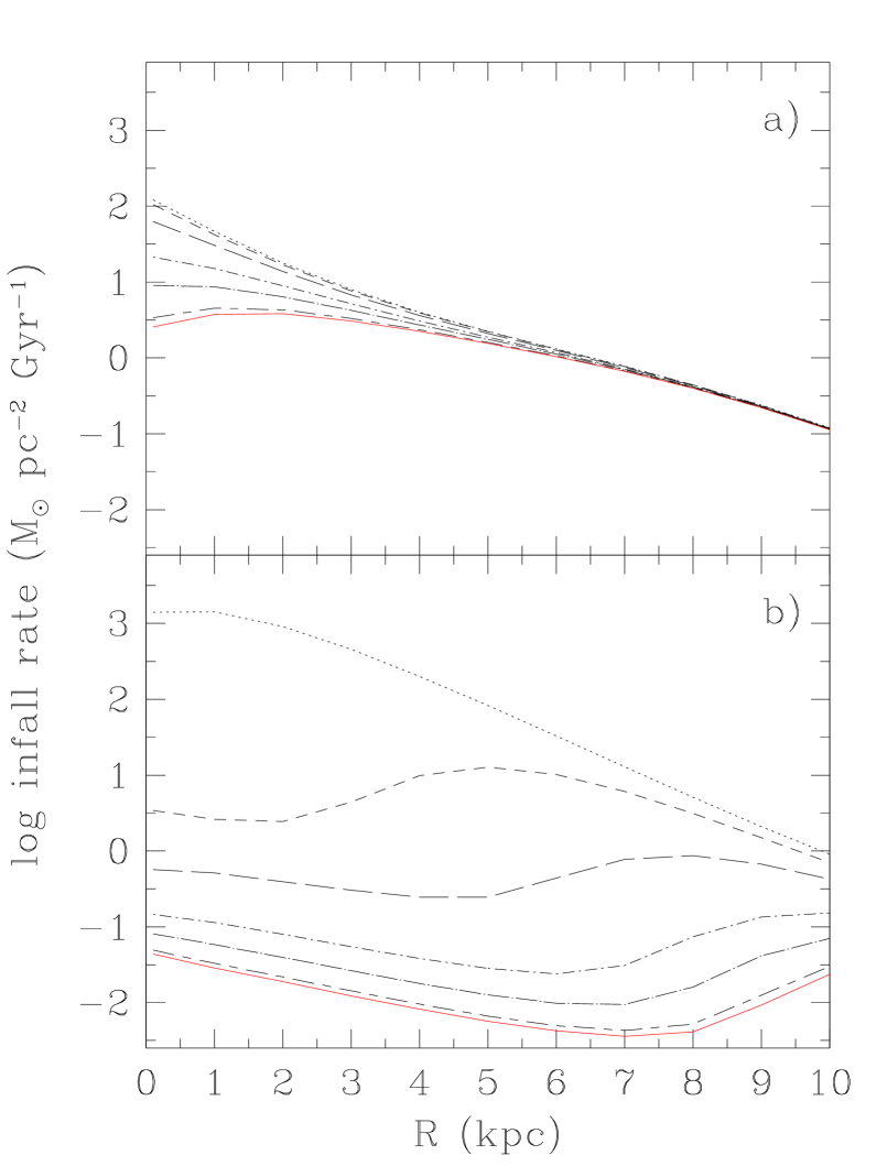
Figure 1: The time evolution of the infall rate for the accretion model (panel a) and for the collapse model (panel b). Curves represents the infall rate at 0.5 (dotted curve), 2 (dashed curve), 3 (long-dashed curve), 5 (dot-dashed curve), 8 (long dash-dotted curve), 12 (long-short dashed curve), and at 13.6 Gyr (solid curve).

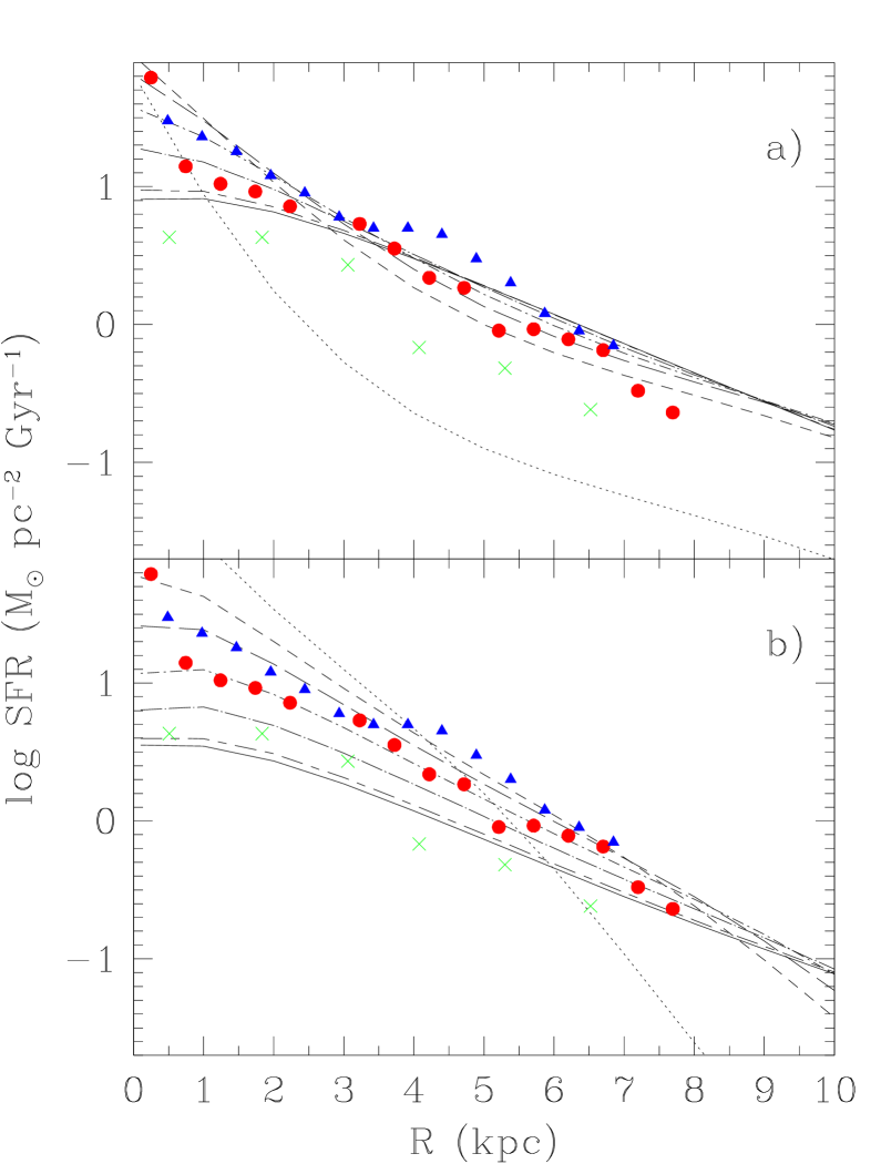
Figure 2: Comparison of the predicted time evolution star formation rate (line types as in Fig.1) with observations for the accretion model (panel a) and with the collapse model (panel b). Data are from Kennicutt et al. (kennicutt89 (1989), crosses); Hoopes & Walterbos (hoopes00 (2000), filled circles); Heyer et al. (heyer04 (2004), triangles).

2.4 The infall rate

Star formation in M33 extends much beyond the region where molecular complexes are located. Carbon stars have been found even at larger radii where the drop of the H$\alpha$ flux occurs ($R\approx 6$ kpc, Kennicutt kennicutt89 (1989)). The presence of such an intermediate-age stellar population in the outer disk suggests that accretion of gas is still taking place (Davidge davidge03 (2003); Block et al. block04 (2004), block06 (2006); Rowe et al. rowe05 (2005)) and that the disk of the galaxy is forming inside-out. A likely source of the accreted gas could be the cosmic web (Keres et al. keres05 (2005)), the warm/hot filaments extending between galaxies, where most of the baryons reside.

Is there any evidence that M33 still in the process of accreting mass from the intergalactic medium? A conspicuous cloud of neutral gas infalling into the disk of M33 recently detected at 21-cm by Westmeier et al. (westmeier05 (2005)) supports this picture. The cloud might have been tidally stripped from a distant faint dwarf or dark galaxy (with no associated stellar counterpart) or it might just be gas condensing out of intergalactic medium filaments. This finding confirms that M33 is still in the process of accreting gas to fuel star formation. The gas infall rate over a disk region corresponding to the cloud size is about 2 $M_{\odot}$ pc^-2 Gyr^-1. There are however observational difficulties in estimating the total amount of gas infalling into the M33 disk. Velocities of the infalling clouds are expected to be similar to velocities of high velocity clouds related to the MW disk, and therefore confusion limits our ability to distinguish the two different populations in the small sky area where M33 is located. Any high velocity cloud in projected proximity to the M33 disk, placed at the distance of M33 would result in a much higher infall rate over M33 than what could be inferred for the same cloud if it were closer to us and infalling into the Milky Way (MW) disk. However, the number of high velocity clouds throughout the whole sky is large, and most of them are connected with gas infalling into the MW galaxy. Observational estimates of the infall rates into the MW disk range between 0.1 and 5 $M_{\odot}$ yr^-1 (e.g. Wakker et al. wakker99 (1999); de Boer deboer04 (2004)). Rates $\approx$ 1 $M_{\odot}$ yr^-1 or larger are favoured by considerations on the rapid molecular gas depletion, on the G-dwarf problem, and by some recent evolution models of disc galaxies (e.g. Naab & Ostriker naab06 (2006) and references therein). The total infall rate for M33 is expected to be lower than in the MW because its total mass is lower than the mass of the MW. This consideration applies both to halo gas infall models, which involve the collapse time scale, and to models where the gas starts flowing in from the intergalactic medium (see Section 3.1). Given that quantitative observations of the infall rate over a wide area of M33 and a wide interval of time are difficult to obtain, in Sect. 4 we shall discuss the implications of models characterized by different infall rates.

2.5 Chemical abundances: stars and ISM

Aller (aller42 (1942)) first obtained spectra of Hii regions in M33 and derived a radial gradient of the [Oii]/[Oiii] line ratio, that he attributed to an excitation gradient. Smith (smith75 (1975)), in subsequent spectroscopic study, found clear evidence for a metallicity gradient. Further spectroscopic studies of Hii regions were carried on by Kwitter & Aller (kwitter81 (1981)) and Vilchez et al. (vilchez88 (1988)). Garnett et al. (garnett97 (1997)) using data from previous observations with derived electron temperatures, re-determined the abundances obtaining an overall O/H gradient of $-0.11\pm 0.02$ dex kpc^-1, including the central regions of M33. The steepness of the gradient is however dominated by the innermost data point. Subsequent studies of the metallicity gradient which do not include the central regions obtain a much shallower gradient. Recently, Willner & Nelson-Patel (willner02 (2002)) have derived Ne/H abundances for 25 Hii regions from infrared lines, obtaining a [Ne/H] gradient $-0.034\pm 0.015$ dex kpc^-1, outside $\sim$0.5 kpc from the center. Crockett et al. (crockett06 (2006)), measuring chemical abundances in six Hii regions, have derived a [Ne/H] gradient of $-0.016\pm 0.017$ dex kpc^-1 and a [O/H] gradient of $-0.012\pm 0.011$ dex kpc^-1, much shallower than in previous studies, but at the limit of significance due to the smallness of the sample. All these determinations are consistent with each other and imply that excluding the innermost $\sim$0.5 kpc region where a bulge might be present, the metallicity gradient of Hii regions in the disk of M33 is very shallow.

Chemical abundances of PNe have been derived by Magrini et al. (m04 (2004)) via optical spectroscopy and photoionization modeling. Stellar abundances have been obtained by Herrero et al. (herrero94 (1994)) for AB-type supergiant stars, McCarthy et al. (mccarthy95 (1995)) and Venn et al. (venn98 (1998)) for A-type supergiant stars, Monteverde et al. (monteverde97 (1997), monteverde00 (2000)) and Urbaneja et al. (urbaneja05 (2005)) for B-type supergiant stars. The larger sample by Urbaneja et al. (urbaneja05 (2005)) indicates an [O/H] gradient of $-0.06\pm 0.02$ dex kpc^-1. Very recently the detection of beat Cepheids, which are young intermediate mass stars (Beaulieu et al. beaulieu06 (2006)) allowed the derivation of their metallicity making use of stellar pulsation models and of the mass-luminosity relation. Beaulieu et al. (beaulieu06 (2006)) derived a metallicity gradient of $-0.20$ dex kpc^-1, and inferred an [O/H] gradient $-0.16$ dex kpc^-1. Metallicities of the old stellar population have been obtained via deep CCD photometry and colour-magnitude diagrams by Stephens & Frogel (stephens02 (2002)), Kim et al. (kim02 (2002)) in inner fields, and by Galletti et al. (galletti04 (2004)), Tiede et al. (tiede04 (2004)), Brooks et al. (brooks04 (2004)) and Barker et al. (barker06 (2006)) in outer fields. The [Fe/H] gradient related to the whole RGB stellar population has a slope $-0.07\pm 0.01$ dex kpc^-1 (Barker et al. barker06 (2006)).

3 The model

The GCE model adopted in this work is a generalization of the multi-phase model by Ferrini et al. (ferrini92 (1992)), built for the solar neighborhood, and subsequently extended to the entire MW (Ferrini et al. ferrini94 (1994)), and to other disk galaxies (e.g. Mollá et al. molla96 (1996), molla97 (1997); Mollá & Diaz molla05 (2005)). Here we summarize the main characteristics of the model (see Ferrini et al. ferrini92 (1992) for details).

The galaxy is divided into $N$ coaxial cylindrical annuli with inner and outer galactocentric radii $R_{i}$ ($i=1,N$) and $R_{i+1}$, respectively, mean radius $R_{i+1/2}\equiv(R_{i}+R_{i+1})/2$ and height $h(R_{i+1/2})$. Each annulus is divided into two zones, the halo and the disk, made of diffuse gas $g$, clouds $c$, stars $s$ and stellar remnants $r$. The halo component is intended here quite generally as the primordial baryonic halo, or as material accreted from interactions with small LG galaxies or from the intergalactic medium during the life-time of the galaxy. In the following, a subscript $H$ or $D$ indicates the halo or the disk, respectively. For a spherical halo of radius $R_{N+1}\equiv R_{H}$,

$$h(R_{i+1/2})=(R_{H}^{2}-R_{i+1/2}^{2})^{1/2},$$ (4)

and the halo volume in the $i$–th annulus is then

$$V_{H,i}=\pi(R_{i+1}^{2}-R_{i}^{2})h(R_{i+1/2}).$$ (5)

If $z_{D}$ is the disk scale height (assumed independent on radius), the volume of the disk in each annulus is

$$V_{D,i}=\pi(R_{i+1}^{2}-R_{i}^{2})z_{D}.$$ (6)

At time $t=0$ all the mass of the galaxy is in the form of diffuse gas in the halo. At later times, the mass fraction in the various components is modified by several conversion processes: diffuse gas is converted into clouds, clouds collapse to form stars and are disrupted by massive stars, stars evolve into remnants and return a fraction of their mass to the diffuse gas. The disk of mass $M_{D}(t)$ is formed by continuous infall from the halo of mass $M_{H}(t)$ at a rate

$$\frac{{\rm d}M_{D}}{{\rm d}t}=fM_{H},$$ (7)

where $f$ is a coefficient of the order of the inverse of the infall time scale. Clouds condense out of diffuse gas at a rate $\mu$ and are disrupted by cloud-cloud collisions at a rate $H^{\prime}$,

$$\frac{{\rm d}M_{c}}{{\rm d}t}=\mu M_{g}^{3/2}-H^{\prime}M_{c}^{2},$$ (8)

where $M_{g}(t)$ and $M_{c}(t)$ are the mass fractions of diffuse gas and clouds, respectively. Stars form in the halo and the disk by cloud-cloud collisions at a rate $H$ and by the interactions of massive stars with clouds at a rate $a$,

$$\frac{{\rm d}M_{s}}{{\rm d}t}=HM_{c}^{2}+aM_{s}M_{c}-DM_{s},$$ (9)

where $M_{s}(t)$ is the mass fraction in stars and $D$ is the stellar death rate.

Each annulus is then evolved independently (i.e. without radial mass flows) keeping fixed its total mass from $t=0$ to $t_{\rm gal}=13.6$ Gyr computing the fraction of mass in each component in the two zones, and the chemical composition of the gas (assumed identical for diffuse gas and clouds). The rate coefficients of the model are all assumed to be independent on time but functions of the galactocentric radius $R$. Their radial dependence for a model of the MW is discussed in detail by Ferrini et al. (ferrini94 (1994)), Mollá et al. (molla96 (1996)), and Mollá & Diaz (molla05 (2005)). In general, coefficients representing condensation processes (like e.g. the formation of clouds from diffuse gas), being proportional to the inverse of the dynamical time, scale with the inverse square root of the zone volume, whereas the coefficients of binary processes (like e.g. the formation of stars by cloud-cloud collisions) scale as the inverse of the zone volume; the coefficient of star formation induced by stars is independent on radius.

Distance	840 kpc
Type	Sc II-III
Inclination	$54^{\circ}$
Position angle	$23^{\circ}$
Luminosity	$6.5\times 10^{9}$ $L_{\odot}$
Maximum rotation speed	130 km s-1
Optical radius $R_{\rm opt}$	6.6 kpc
Equivalent Solar radius	3.9 kpc

Table 1: M33: adopted physical characteristics

The model described in this section can be applied in general to study the chemical evolution of any disk galaxy. We now discuss the values of the various coefficients that we have specifically adopted for M33. As a starting point, we have adopted the set of values by Ferrini et al. (ferrini92 (1992)) for their “best model” of the solar neighborhood, applying them at the equivalent solar radius . The values at any other radius are then determined by the scaling relations described in Sect. 3.

The mass fractions in each component computed by the model in each annulus are then converted into surface densities using as a normalization the total surface density, (i.e. the sum of the Hi, H₂, stellar and remnants surface densities, as given by equations 1 and 2). In the comparison with the data, we identify the gas and cloud components with the Hi and the H₂ gas, respectively.

3.1 The infall coefficient

We assume an exponential radial dependence of the infall rate $f$,

$$f(R)=f_{0}\exp(-R/\lambda_{D})$$ (10)

where $f_{0}$ is the infall rate at $R=0$ and $\lambda_{D}$ is a typical disk scale length (cf. Ferrini et al. ferrini94 (1994), Portinari & Chiosi portinari99 (1999)). In principle, $\lambda_{D}$ can be set equal to the scale length of the disk surface brightness in the $B$-band ($\sim 1.9$ kpc, Freeman freeman70 (1970)), or in the $K$-band ($\sim 1.4$ kpc, Regan & Vogel regan94 (1994)), or to the CO scale length ($\sim 2.7$ kpc, Corbelli corbelli03 (2003)). In our model, the value of $\lambda_{D}$ that better reproduces the observations (gas and stars surface density profiles, radial SFR, see Figs. 2, 3, 4, 5) is $\lambda_{D}\approx 2.0$ kpc. Larger values of $\lambda_{D}$ imply a huge amount of neutral hydrogen in the central regions, while lower values depress the SFR in the inner regions.

The infall coefficient $f_{0}$ is usually set of the order of the inverse of the collapse time $\tau_{c}$ for the galaxy, where $\tau_{c}$ depends on the total mass of the galaxy $M_{\rm Gal}$ as $\tau_{c}\propto M_{\rm Gal}^{-1/2}$ (Gallagher et al. gallagher84 (1984)). This choice corresponds to a scenario where the disk is formed very rapidly at the beginning of a galaxy’s life and we shall refer to this model as the collapse model. Since the mass of M33 is about 0.2 times the mass of the MW, the value of $f_{0}$ for M33 should be a factor $\sim 2.2$ smaller than in the case of the MW. Scaling the infall value adopted by Ferrini et al. (ferrini92 (1992)) for the MW ($f_{0}=0.7$ see Table 2), corresponding to a dynamical collapse time of the order of 10⁸ yr at the solar radius, we obtain for M33 $f_{0}\approx 0.3$. Over a disk of 10 kpc in radius this choice results in a present-day average accretion rate of $\dot{M}_{\rm inf}\approx 0.05$ $M_{\odot}$ pc^-2 Gyr^-1 (Fig 1b). Thus our collapse model is intended to reproduce the characteristics of a rapid phase of disk formation, following the dynamical collapse of an extended halo.

However, estimates of $f_{0}$ for the MW based on chemical constraints (G-dwarfs metallicity distribution, O/Fe vs. Fe/H relations, etc.) suggest lower values, $f_{0}\approx 0.012$ for the MW, corresponding to a time scale of the order of several Gyr (see Mollá & Diaz molla05 (2005) and references therein). Lower values of $f_{0}$ implies higher infall rates at the present time. If this is the case for M33 it is unlikely however that the halo is the reservoir of the gas infalling into the disk because there are no observational evidences for a gaseous halo. A possibility for supporting a high infall rate at present time, and in general an infall rate almost constant in time, is to consider a slow continuous accretion process from the environment. This is obtained for example using $f_{0}\approx 0.003$, corresponding to an infall rate of 1.2 M_⊙ yr^-1 in the M33 disk at present time or about and average of $\dot{M}_{\rm inf}\approx 3.8$ $M_{\odot}$ pc^-2 Gyr^-1 (Fig 1a). We shall refer to this model as the accretion model.

High infall rates are favoured by some recent papers describing the evolution of disk galaxies (e.g. Naab & Ostriker naab06 (2006)). Infall rate in the MW for example are predicted to be of order 2–4 M_⊙ yr^-1, with little variations over the last 10 Gyr. These values are in good agreement with those inferred from observations of high velocity clouds and explain specific abundance patterns such as the high deuterium abundance at the solar neighborhood and at the Galactic Center (Chiappini et al. chiappini02 (2001)). In these models the intergalactic medium is often identified as the source of the gas infalling into the disk. Hydrodynamical simulations of galaxy formation and evolution predict that accretion of ‘cold’ gas from intergalactic filaments is present and becomes the dominant process for low mass galaxies and in low density regions. Galaxies of mass similar to M33 should accrete gas at a rate which decreases slowly with time and is currently $\approx$ 1 $M_{\odot}$ yr^-1 (Keres et al. keres05 (2005)). This finding supports the infall rates used in our accretion model. Higher mass halos have larger accretion rates but a large fraction of the accreted gas has been shock heated at the time the galaxy formed, and does not flow in from large distances, as in the case of intergalactic filaments feeding the disk. The intergalactic feeding mechanism is well suited for M33 because of the absence of a massive gaseous and stellar halo, relic of the galaxy formation epoch and driver of disk accretion processes.

3.2 The star and cloud formation efficiencies

The parameters regulating the conversion of diffuse gas into clouds and clouds into stars are: $\mu$ (cloud formation from diffuse gas), $H$ (star formation from cloud collisions), and $H^{\prime}$ (cloud dispersion). The efficiencies of these processes adopted in our models, together with previous values adopted for the MW and M33, are shown in Table 2. These efficiencies are in general functions of the morphological type of the galaxy (cf. Sandage sandage86 (1986); Gallagher et al. gallagher84 (1984)); Ferrini & Galli (ferrini88 (1988)) analyzed the behaviour of these parameters in the different morphological types of spiral galaxies, and found a reduction of $\mu$ and $H$ from a Sbc galaxy, like the MW, to a Scd galaxy, like M33. These scaling relations can be also compared with those of Mollá & Diaz (molla05 (2005)) who studied spiral galaxies of different morphological types. For a spiral galaxy of morphological type 6, such as M33, they adopted the following values (see their Table 2): $\epsilon_{H}=0.01$ and $\epsilon_{\mu}=0.15$, which translate, at the equivalent solar radius, into $H=0.012$ and $\mu=0.017$ in units of 10^-7 yr^-1, using the relations between $\epsilon_{H}$, and $H$ and between $\epsilon_{\mu}$ and $\mu$ given by Ferrini et al. (ferrini94 (1994)). The $H$ parameter adopted in the present work, in particular for the accretion model, has a higher value than that used for M33 by Mollá & Diaz (molla05 (2005)) and by Mollà et al. (molla96 (1996),molla97 (1997)). This is probably due to the different parameterization of the IMF used: Mollà and collaborators used the Ferrini’s et al. (ferrini90 (1990)) IMF which predicts a larger number of massive stars with respect to other IMF, such as the Kroupa’s et al. (kroupa93 (1993)) IMF. Therefore their model needed a lower $H$ value in order to reproduce the observed metal content.

Note that in order to reproduce the observed lower content of molecular gas (Fig. 5) of M33 with respect to that found in Sc galaxies, a very low cloud formation efficiency is needed. The low molecular fraction in this galaxy is in agreement with the tendency of the gas fraction in molecular form to decrease from Sc to Irr morphological types, despite the higher SFR of the latter.

3.3 The cloud dispersal coefficient

The cloud dispersal coefficient $H^{\prime}$ is a measure of the probability that collisions between gas clouds result in the disruption of the clouds themselves and return cloud material to the diffuse phase. In principle, the rate of cloud dispersal should depend on radius in the same way as the rate of star formation by cloud-cloud collisions, namely as the inverse of the disk volume $V_{D}$ (see Ferrini et al. ferrini94 (1994)). However, this dependence makes impossible to reproduce the observed distributions of Hi and H₂, because at small galactocentric radii, where the factor $1/V_{D}$ enhances the rate of formation of diffuse gas by cloud collisions, the Hi gas is underabundant (see Fig. 4). Our model requires instead that the coefficient of cloud dispersal, $H^{\prime}$, should be roughly independent on radius. Since the dependence of the frequency of collisions from the inverse of the volume is a general characteristic of any binary collision process, an additional hypothesis must be made about the efficiency of the process of cloud dispersal. Namely, our modeling requires that the clouds in the outer galaxy are more efficiently dispersed by collisions than clouds in the inner galaxy.

This model requirement is related to the observed absence of GMCs at large radii where star formation is still taking place, supporting the claim that clouds are easily destroyed in the outer disk of M33. This may be due to a radial change of some intrinsic property of the clouds (e.g. compactness) or to additional processes that regulate the molecular/atomic hydrogen ratio in galaxies of low molecular fraction such as M33, like photodissociation by a pervasive interstellar radiation field (Elmegreen elmegreen93 (1993); Heyer et al. heyer04 (2004)). Because of the larger photon mean free path at larger radii, this process probably dominates the conversion of molecular clouds into atomic diffuse gas in the outer disk of M33.

3.4 Stellar yields

We model the chemical enrichment of the gas using the formalism developed by Talbot & Arnett (talbot73 (1973)) who introduced the restitution matrices $Q_{i,j}(M,Z)$. The elements of these matrices are defined as the fraction of the mass of an element $j$ initially present in a star of mass $M$ and metallicity $Z$ that it is converted in an element $i$ and ejected. At each stellar mass $M$ and metallicity $Z$ corresponds one matrix $Q_{i,j}(M,Z)$. Our GCE model takes into account two different metallicities, $Z=0.02$ and $Z=0.006$, and 22 stellar masses (21 for $Z=0.006$), ranging from 0.8 to 100 $M_{\odot}$, for a total of 43 restitution matrices.

We update the nucleosynthesis yields used to build the $Q_{i,j}(M,Z)$ matrices in the following way. For low- and intermediate-mass stars ($M<8$ $M_{\odot}$) we use the yields by Gavilán et al. (gavilan05 (2005)) for both values of the metallicity. We have also tried the yields of Marigo (marigo01 (2001)), which however do not give any appreciable difference in the computed gradients of chemical elements produced by intermediate mass stars, as N. For stars in the mass range $8\leavevmode\nobreak\ M_{\odot}<M<35\leavevmode\nobreak\ M_{\odot}$ we adopt the yields by Chieffi & Limongi (chieffi04 (2004)) for $Z=0.006$ and $Z=0.02$. The yields of more massive stars are affected by considerable uncertainties associated to different assumptions about the modeling of processes like convection, semiconvection, overshooting, mass loss. Other difficulties arise from the simulation of the supernova explosion and the possible fallback after the explosion, that strongly influences the production of iron-peak elements. It is not surprising then that the results of different authors (e.g. Arnett arnett95 (1995); Woosley & Weaver woosley95 (1995); Thielemann et al. thielemann96 (1996); Aubert et al. aubert96 (1996)) disagree in some cases by orders of magnitude . In our models, we estimate the yields of stars in the mass range $35\leavevmode\nobreak\ M_{\odot}<M<100\leavevmode\nobreak\ M_{\odot}$ by linear extrapolation of the yields in the mass range $8\leavevmode\nobreak\ M_{\odot}<M<35\leavevmode\nobreak\ M_{\odot}$.

3.5 The IMF

Recent work supports the idea that the IMF is universal in space and constant in time (Wyse wyse97 (1997); Scalo scalo98 (1998); Kroupa kroupa02 (2002)), apart from local fluctuations. As reviewed by Romano et al. (romano05 (2005)) there are several parameterizations of the IMF that have been used in GCE models, starting from the original Salpeter (salpeter55 (1955)) power-law: piecewise power-laws (Tinsley tinsley80 (1980); Scalo scalo86 (1986); Kroupa et al. kroupa93 (1993); Scalo scalo98 (1998)), polynomial approximations (Ferrini et al. ferrini90 (1990)), and logarithmic polynomials (Chabrier chabrier03 (2003)). Romano et al. (romano05 (2005)) studied the sensitivity of GCE models to different parameterizations of the IMF and found that the Scalo (scalo86 (1986)), Kroupa et al. (kroupa93 (1993)) and Chabrier (chabrier03 (2003)) IMFs are generally more consistent with observational data than those of Salpeter (salpeter55 (1955)) and Scalo (scalo98 (1998)).

One of the results most sensitive to the choice of the IMF is the metallicity gradient in the disk. In fact, the magnitude and the slope of chemical abundance gradients are related to the number of stars in each mass range, and so to the IMF. With our set of chemical yields (see Sect. 3.4), we find the best agreement with the observed gradients adopting a two power-law IMF analogous to Kroupa’s IMF (with a slope $-2.35$ for $M>1$ $M_{\odot}$ and $-1.2$ for $M<1$ $M_{\odot}$). This is the IMF adopted in this work. Other parameterizations, with the exception of Chabrier’s IMF, result in general in an under-production of massive stars, and, consequently, a lower production of metals.

We also examine the effects of a possible dependence of the slope of the IMF on galactocentric radius. On the basis of HST photometric observations of stellar clusters embedded in several giant Hii regions of M33, Lee et al. (lee02 (2002)) found that the IMF becomes steeper (less rich in massive stars) with increasing galactocentric radius and decreasing metal abundance. Assuming a variable slope in the range $10\leavevmode\nobreak\ M_{\odot}<M_{\odot}<100\leavevmode\nobreak\ M_{\odot}$ as suggested by Lee et al. (lee02 (2002)), we find however that the resulting metallicity gradient is not consistent with the observations, being characterized by a much shorter scale length than the observed distribution of metals.

4 Results of the model

	$R_{D}$	$R_{H}$	$\lambda_{D}$	$H(R_{\odot,{\rm M33}}$)	$H^{\prime}(R_{\odot,{\rm M33}}$)	$\mu(R_{\odot,{\rm M33}}$)	$f_{0}$	ref.
	(kpc)	(kpc)	(kpc)	(107  yr)-1	(107 yr)-1	(107  yr) -1	(107  yr)-1
M33	0.2	20	2	0.2	0.2	0.01	0.003	a
M33	0.2	20	2	0.06	0.2	0.01	0.3	b
Spiral $N=6$	–	–	–	0.012	–	0.017	0.009	c
M33	–	–	–	0.006	–	0.006	0.0056	d
MW	–	–	2	0.5	1.0	0.05	0.7	e

Table 2: Parameters of the GCE models for M33 and the MW. $H$, $H^{\prime}$ and $\mu$ are given at the equivalent solar radius ($R_{\odot,{\rm M33}}$), $f_{0}$ is given at the centre. References: a, accretion (this work); b, collapse (this work); c, Mollá & Diaz (molla05 (2005)) for a spiral galaxy of morphological type $N=6$; d, Mollá et al. (molla96 (1996), molla97 (1997)), e Ferrini et al. (ferrini92 (1992)) for the MW.

In this section we present the results of our GCE model for M33 described in Sect. 3, and compare them to the data discussed in Sect. 2. In particular, we examine the SFR, the distribution of atomic and molecular gas, and the chemical abundance gradients.

4.1 The evolution of the SFR

An important constraint to GCE models is the magnitude and the radial profile of the SFR at the present epoch. This observable allows one to discriminate between different evolutionary scenarios that result in the same radial distributions of stars, gas and chemical abundances.

This is illustrated by the two models presented in Fig. 1 and in Table 2, labeled collapse and accretion, differing in the time behavior of the accretion rate on the disk. In the former, the disk is formed by the collapse of the gas initially present in the galaxy’s halo, and the resulting accretion rate of the disk decreases rapidly with time (Fig. 1), simulating a rapid collapse phase. Since the exponential time scale of collapse is longer for the outer, less dense, regions of the halo, the disk is formed in an inside-out fashion, as clearly shown by the radial profile of the infall rate in Fig. 1b. In the accretion model, the infall rate is approximately constant for the entire evolution of the galaxy (except the inner few kpc, where it decreases by about one order of magnitude). In this case, the disk of M33 is built by continuous gas supply from the external medium, a process supporting a substantial star formation at all radii, in agreement with the observations discussed in Sec. 2.4.

Both models well reproduce the present time atomic and molecular gas distributions, and the stellar density profile of M33. The differences between the two models are evident at earlier times, because the bulk of the stellar mass settles in the disk earlier in the collapse model than in the accretion model, due to the rapid gas infall and to the high star formation rate. The behaviour of the SFR reflects the differences in the two models at the present time: the actual SFR predicted by the accretion model is in closer agreement with the observations than the SFR predicted by the collapse model. In the collapse model the accretion rate and SFR vary more rapidly with time: as a consequence stars form earlier and the present-day SFR is at least a factor $\sim 3$ lower than what can be inferred by infrared and optical observations. Clearly, the higher infall rate on the disk at present times for the accretion model results in a more vigorous SFR than in the collapse model. But at earlier times the SFR was higher for the collapse model, since the larger gas reservoir accreted earlier by the disk was converted into stars. The present-day SFR integrated over the disk up to $R=10$ kpc is $0.2$ $M_{\odot}$ yr^-1 for the collapse model and $0.5$ $M_{\odot}$ yr^-1 for the accretion model, but the difference increases in the inner regions of the disk. The integral of the observed SFR up to $R=7$ kpc, $\sim 0.4$ $M_{\odot}$ yr^-1 (see Sect. 2.3), is in good agreement with the accretion model results. Also the intermediate-age SFR derived from PNe, $\sim 0.55$ $M_{\odot}$ yr^-1 from 1 to 4 Gyr ago, and $\sim 1.1$ $M_{\odot}$ yr^-1 from 1 to 8 Gyr ago, are in closer agreement with the accretion model which predicts $0.7$ $M_{\odot}$ yr^-1 and $0.9$ $M_{\odot}$ yr^-1 respectively. In the rest of the paper we adopt the accretion model to describe the evolution of M33.

4.2 The radial distribution of gas and stars

We show in Figures 3, 4, 5, the time evolution of the surface densities of stars, atomic, and molecular gas. The diffuse gas is accreted by the disk from the external medium following an exponential law which produces a larger amount of gas in the central regions of the galaxy. Clouds form out of this diffuse gas, whose surface density decreases with time. Stars are formed at the expense of clouds, and the cloud surface density decreases with time while the stellar surface density increases. The present-time radial distribution of diffuse and condensed gas can be compared with the observed radial profiles of atomic and molecular gas, respectively. The model predicts a slightly higher surface density of diffuse gas in the central regions and a lower cloud surface density than observed. This might either imply that the formation of diffuse gas via clouds collisions is even more inefficient at small radii than we assumed, or that there is an enhanced formation of molecular clouds. This might be due to additional features in place in the central regions, such as a small bar fueling gas towards the center or to a small bulge with a higher metal and dust abundance enhancing the molecular hydrogen fraction. The slightly lower abundance of clouds seen at large galactic radii might be associated with a change of the CO-H₂ conversion factor due to, e.g. a lower excitation rate of the CO molecule.

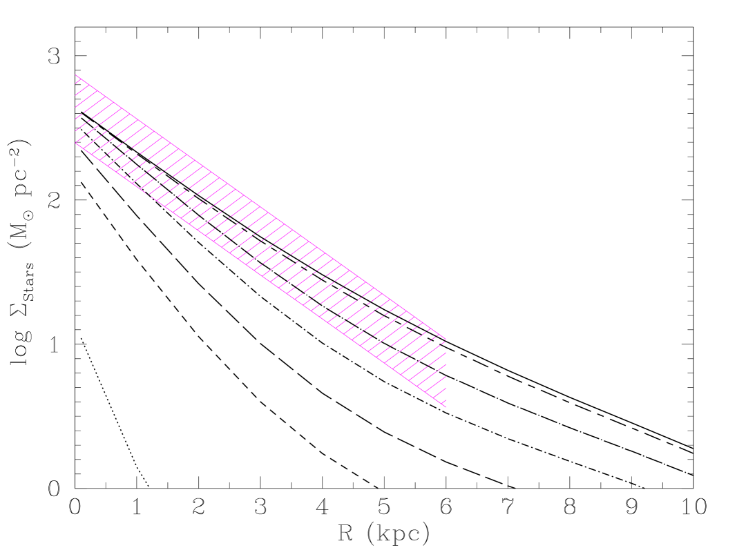
Figure 3: Time evolution of the stellar surface density (line types as in Fig. 2), compared with the stellar surface density determined by Corbelli (corbelli03 (2003), shaded region).

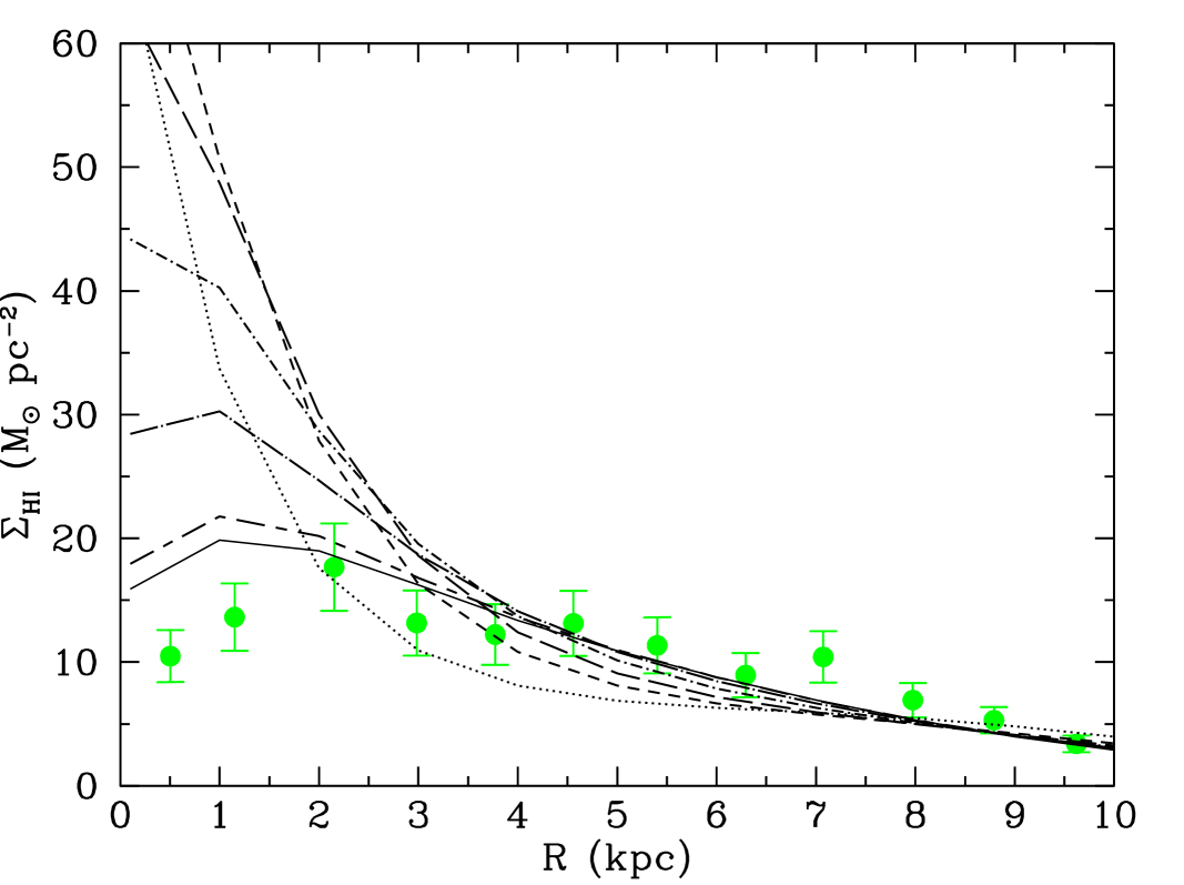
Figure 4: Time evolution of the surface density of diffuse gas (line types as in Fig. 2), compared with the observed surface density of atomic hydrogen (Corbelli corbelli03 (2003)).

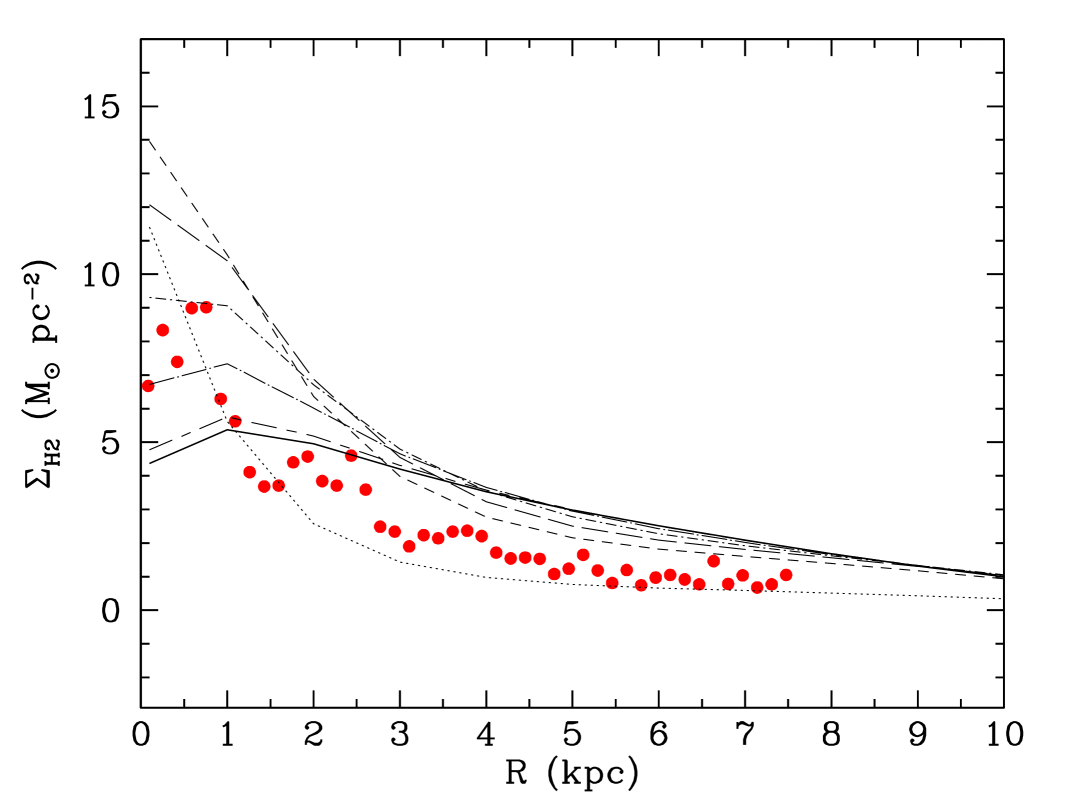
Figure 5: Time evolution of the surface density of clouds (line types as in Fig. 2), compared with the observed surface density of molecular hydrogen (Corbelli corbelli03 (2003)).

4.3 The metallicity gradients

We now examine the evolution of the abundance gradients of O, Ne, S, N, and Fe in M33. In this nearby galaxy is possible to separate the present-day metallicity gradient, outlined by abundances of HII regions, A-type and B-type supergiant, and Cepheids, from an older metallicity gradient, outlined by PNe and RGB stars. The PNe trace the chemical composition of the ISM over a range of galactic ages between $\sim 1$ to $\sim 8$ Gyr ago, at least for those elements not affected by stellar evolution in the mass range $M<$8 M_⊙, such as O, Ne (only as a first approximation, cf. Marigo marigo01 (2001); Magrini et al. 2005a ), and S. Abundances in RBG stars trace the metallicity gradient relative to an even distant past ($>$8 Gyr ago).

In order to avoid statistical effects due to the incompleteness of the various samples, in the rest of this Section we shall compare the model results with larger and homogeneous samples of chemical abundance determinations for each class of objects, namely Hii regions, young stars, and RGB stars. As discussed by e.g Vilchez et al. (vilchez88 (1988)), Urbaneja et al. (urbaneja05 (2005)), Magrini et al. (m07 (2007)), the gradient in M33 does not have not a constant slope, and it cannot be represented by a single power-law: studies undertaken for different radial ranges would produce different results. Inclusion of the innermost regions would result in a steeper gradient. On the contrary the gradient flattens out if only regions far from the center were considered. Thus, for each chemical element we compute the gradient considering all data from the literature within a given radial range, and we include also new abundance determinations by Magrini et al. (m07 (2007)). In Table 3 we list the slope of the gradients and the references for the data used to derive it.

	Model			Observations			References
	Present	5 Gyr ago	8 Gyr ago	Hii regions	young stars	PNe	RGB	Hii regions	young stars	PNe	RGB
				present time		1-8 Gyr ago	$>8$ Gyr
O/H	$-0.067$	$-0.078$	$-0.094$	$-0.07\pm 0.01$	$-0.07\pm 0.02$	$-0.11\pm 0.05$		a, b, c	g, h, k	j
								d, e
Ne/H	$-0.067$	$-0.077$	$-0.091$	$-0.06\pm 0.02$				f, d		j
S/H	$-0.072$	$-0.082$	$-0.095$	$-0.07\pm 0.05$		$-0.09\pm 0.04$		b, c, e
N/H	$-0.125$	$-0.137$	$-0.149$	$-0.10\pm 0.02$				a, b, c, e
Fe/H	$-0.062$	$-0.069$	$-0.080$				$-0.07\pm 0.01$				i, l, m
											n, o, p

Table 3: Metallicity gradients (dex kpc^-1) from 1 to 10 kpc. The observed gradients are computed from the data discussed in Sect. 2.5 using a weighted linear fit. Model gradients are approximated by linear fits. References: a, Smith (smith75 (1975)); b, Kwitter & Aller (kwitter81 (1981)); c, Vilchez et al. (vilchez88 (1988)); d, Crockett et al. (crockett06 (2006)); e, Magrini et al. (m07 (2007)); f, Willner & Nelson-Patel (willner02 (2002)); g, Monteverde et al. (monteverde97 (1997), monteverde00 (2000)); h, Urbaneja et al. (urbaneja05 (2005)); k, Beaulieu et al. (beaulieu06 (2006)); j, Magrini et al. (m04 (2004)); i, Barker et al. (barker06 (2006)); l, Stephens & Frogel (stephens02 (2002)); m, Kim et al. (kim02 (2002)); n, Galletti et al. (galletti04 (2004)); o, Tiede et al. (tiede04 (2004)); p, Brooks et al. (brooks04 (2004)).

4.3.1 The abundance of oxygen

In Fig. 6 we compare the time evolution of the O gradient with observations of Hii regions ($a$), stars ($b$) and PNe ($c$). The O/H gradient predicted by the model at present time is $-0.067$ dex kpc^-1 from 1 to 10 kpc in radius. This is in agreement with the gradient derived in the same radial range from a combined sample composed by abundances in Hii regions available in the literature and from recently acquired data presented in Magrini et al. (m07 (2007)). A linear fit of all H ii regions data, which references are quoted in Table 3, gives $-0.07\pm 0.01$ dex kpc^-1 over a range of radii from 1 to 10 kpc, even though the data show that the gradient flattens out going radially outwards. We stress the need to assemble a statistically significant sample in order to avoid the influence of intrinsic peculiarities of the observed sources and inhomogeneities associated to particular regions e.g. to spiral arms.

The correspondence between the predicted O/H gradient and that determined from absorption lines in young stars is also very good. Monteverde et al. (monteverde00 (2000)) find $-0.078\pm 0.06$ dex kpc^-1, and a similar value was also found by Urbaneja et al. (urbaneja05 (2005)), $-0.06\pm 0.02$ dex kpc^-1. The overall linear fit to O abundances from young stars, including A, B giant stars and Cepheids, (references quoted in Table 3), gives $-0.07\pm 0.02$ dex kpc^-1 (Pearson correlation factor $-0.6$), in agreement with the model result (see Table 3).

The O/H gradient of a sample of PNe reaches a lower absolute value of abundances at large radii and is steeper than the O/H gradient outlined by Hii regions and young stars. A weighted linear fit gives a slope $-0.10\pm 0.05$ dex kpc^-1 (with Pearson correlation factor $-0.7$). This behaviour is expected in a scenario where metallicity gradients flatten with time because chemical abundances at large radii increase gradually with time while the enrichment process is very fast in the central regions. The O/H gradient from PNe is representative of the metallicity in the disk of M33 about 1–8 Gyr ago. The same is shown by our model (compare the long-short dashed curve and the short dash-dotted line in Fig.6$c$). More quantitatively, the slopes of the O/H gradients predicted by our model are $-0.078$ dex kpc^-1 and $-0.094$ dex kpc^-1, 5 and 8 Gyr ago respectively (see Table 3).

Our sample includes some of the brightest PNe of M33, probably representative of a younger population than the average sample (Richer et al. richer98 (1998)). Five PNe show an O abundance in agreement with the model predictions, four are marginally consistent, and two are over-abundant in O (PN 75 and 91, see Magrini et al. m04 (2004)). A possible explanation for the O over-abundance in some PNe is the occurrence of hot bottom burning and third dredge-up processes during the post-AGB phases, with a consequent O enrichment in the nebula (Marigo marigo01 (2001), Herwig herwig04 (2004)). These processes are generally associated with massive progenitors and therefore with N enrichment as well. We have therefore excluded the two PNe over-abundant in O from the weighted linear fit shown in Table 3.

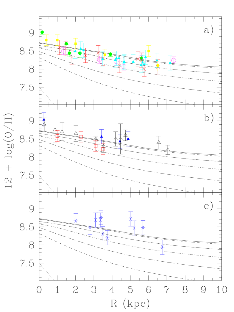
Figure 6: The time evolution of the O gradient (line types as in Fig. 2) compared with: a) Hii region determinations: Smith (smith75 (1975), filled squares); Kwitter & Aller (kwitter81 (1981), crosses); Vilchez et al. (vilchez88 (1988), filled circles); Crockett et al. (crockett06 (2006), empty circles); Magrini et al. (m07 (2007), filled triangles); b) B supergiant stars: Monteverde et al. (monteverde97 (1997), monteverde00 (2000), filled triangles); Urbaneja et al. (urbaneja05 (2005), empty triangles); Cepheids: Beaulieu et al. (beaulieu06 (2006), empty squares); c) PNe abundances: Magrini et al. (m04 (2004), crosses).

4.3.2 The abundance of neon

O and Ne are both produced mainly by short-lived, massive stars ($M>10$ $M_{\odot}$). Stellar nucleosynthesis models (e.g. Chieffi & Limongi chieffi04 (2004), Hirschi et al. hirschi05 (2005)), predict that the abundances of these two elements should be closely correlated. This prediction is supported by abundance measurements in Galactic and extragalactic PNe (Henry henry90 (1990)), showing that Ne/O is constant over a wide range of [O/H] values. Fig.6 and 7, show indeed that the slopes of the two gradients predicted by our model are indistinguishable and equal to $-0.067$ dex kpc^-1.

Willner & Nelson-Patel (willner02 (2002)) derived the Ne abundance for 25 Hii regions in M33 from infrared spectroscopy. They find an inconsistency with the O gradient measured by Vilchez et al. (vilchez88 (1988), $-0.12\pm 0.01$ dex kpc^-1. Excluding the inner two and the outer three regions of their sample they found a best-fit slope of $-0.07\pm 0.02$ dex kpc^-1, in agreement with our predictions. An even shallower slope for the [Ne/H] gradient is found by Crockett et al. (crockett06 (2006)), $-0.016$ dex kpc^-1. Both sets of observations are plotted in Fig.7 for a comparison with our predicted gradient. Although there is some dispersion in the data in the central and outer regions, the overall slope of the observed Ne/H gradient is $-0.06\pm 0.02$ dex kpc^-1 (with Pearson correlation factor $-0.7$). This has been computed using data available in references given in Table 3, and is in agreement with the gradient of $-0.067$ dex kpc^-1 predicted by our model.

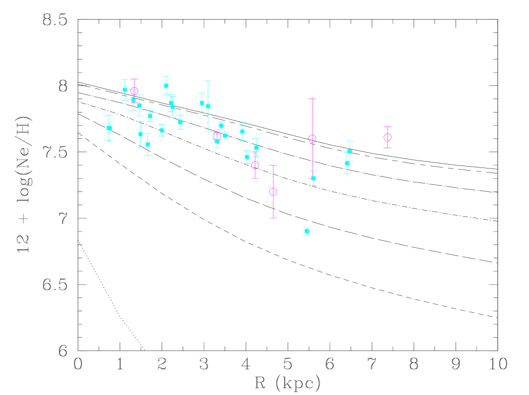
Figure 7: The time evolution of the Ne gradient (line types as in Fig.2). Comparison with the observations: Hii regions infrared spectra, Willner & Nelson-Patel (willner02 (2002), filled squares) and optical spectra, Crockett et al. (crockett06 (2006), empty circles).

4.3.3 The abundance of sulfur

The abundance of S in PNe is expected to be a better tracer of the chemical composition of the ISM at the time of formation of PNe progenitors than the abundance of O and Ne (Henry et al. henry04 (2004)). For this reason, the S/H gradient in PNe has been used in our Galaxy to determine the temporal behaviour of the metallicity gradient (Maciel et al. maciel05 (2005), maciel06 (2006)). We recall however the possible sulfur “anomaly” seen in some Galactic PNe (Henry et al. henry04 (2004)): when compared with similar data for stars and Hii regions, some Galactic PNe have much lower S abundance than expected on the basis of their O abundance. This anomaly is not dominant in the sample of PNe by Magrini et al. (m04 (2004)). The average $\log({\rm S/O})=-1.92$ is consistent with Galactic studies of both PNe and Hii regions (cf. $-1.91\pm 0.24$, Henry et al. henry04 (2004)). It might be present at most in two PNe (PN93 and PN96) with very low S/O ratio.

In Fig.8a and b we show the S abundance of Hii regions and PNe, respectively. Notice the good agreement of the present-day S gradient predicted by our model ($-0.07$ dex kpc^-1), with the S abundances gradient for Hii regions ($-0.07\pm 0.05$ dex kpc^-1, Pearson correlation factor of $-0.6$). A best-fit to the PN sample gives an S gradient of $-0.09\pm 0.04$ dex kpc^-1 (with a Pearson correlation factor $-0.8$) consistent with the value $-0.082$ dex kpc^-1 predicted by our model 5 Gyr ago. We have excluded the two PNe possibly affected by the sulfur “anomaly”. These do not correspond to the two PNe excluded from the oxygen gradient, since the two phenomena, sulfur “anomaly” and oxygen overabundance, are not necessarily linked.

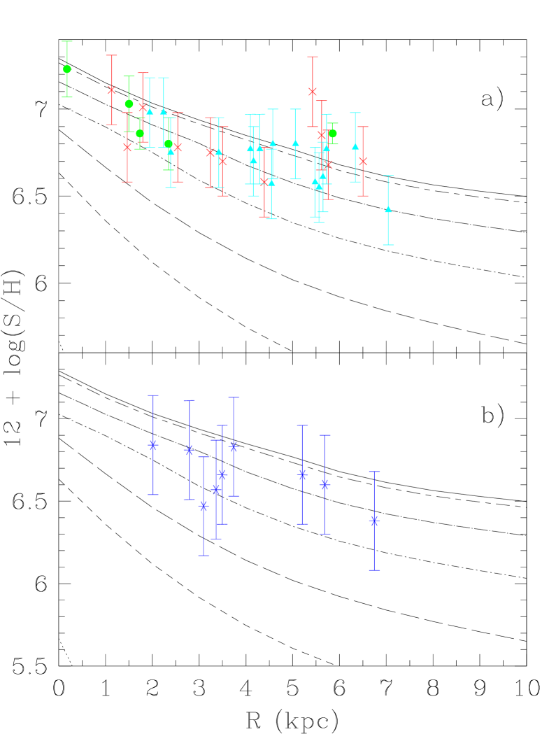
Figure 8: The time evolution of the S gradients (line types as in Fig.2) compared with the observations of: a) Hii regions: Kwitter & Aller (kwitter81 (1981), crosses); Vilchez et al. (vilchez88 (1988), filled circles); Magrini et al. (m07 (2007), filled triangles); b) PNe: Magrini et al. (m04 (2004), crosses).

4.3.4 The abundance of nitrogen

Unlike O, Ne and S, nitrogen is mainly produced by intermediate mass stars. Therefore, the N abundance of B stars (Urbaneja et al. urbaneja05 (2005)) and PNe (Magrini et al. m04 (2004)) is affected by nucleosynthesis processes, and cannot be used to infer the original chemical composition of the ISM. In Fig.9 we show the model evolution of the N/H gradient and the abundances observed in Hii regions. The predicted slope of the present-day N gradient, $-0.125$ dex kpc^-1, is in good agreement with Hii regions data ($-0.10\pm 0.02$ dex kpc^-1, with a Pearson correlation factor $-0.8$).

The general agreement of the observed gradients of chemical elements produced by stars in different mass ranges with the model supports the reliability of the adopted IMF. Any choice of the IMF that predicts the correct number of massive stars, but not of low- and intermediate mass stars, would reproduce equally well the O/H, S/H and Ne/H gradients, but would fail in predicting the N radial distribution.

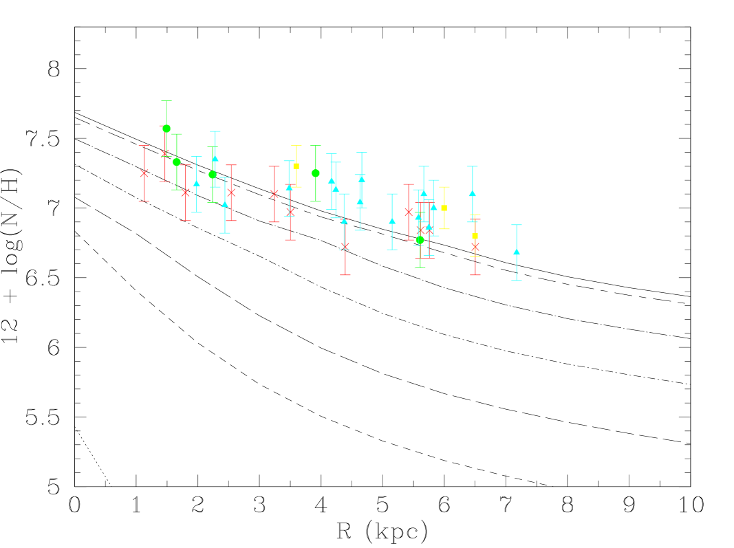
Figure 9: The time evolution of the N/H gradient according to our model (line types as in Fig. 2), compared with measurements of N in Hii regions: Smith (smith75 (1975), filled squares); Kwitter & Aller (kwitter81 (1981), crosses); Vilchez et al. (vilchez88 (1988), filled circles); Magrini et al. (m07 (2007), triangles).

4.3.5 The abundance of iron

Barker et al. (barker06 (2006)) analyzed [Fe/H] abundances in RGB stars of M33 from new observations and from previous works by Stephens & Frogel (stephens02 (2002)), Kim et al. (kim02 (2002)), Galletti et al. (galletti04 (2004)), Tiede et al. (tiede04 (2004)), Brooks et al. (brooks04 (2004)). Using these data, they found a well defined gradient $[{\rm Fe/H}]=-0.07R-0.49$ extending up to $R\approx 12$ kpc. Fig.10, shows the good agreement between the time evolution of Fe/H predicted by our model and the RGB abundances of Barker et al. (barker06 (2006)). The epoch of formation of RGB stars is $>$8 Gyr ago, when the slope of the Fe/H gradient according to our model is $-0.08$ dex kpc^-1. Note however that the linear fit is a very rough approximation to the effective model gradient.

The metallicity gradient of Cepheids determined by Beaulieu et al. beaulieu06 (2006), -0.2 dex kpc^-1, can also be compared with the predicted gradient at present time. However, the five observed Cepheids are located in the radial region from $\sim$1 to 4 kpc, whereas our computed gradient extends out to 10 kpc. In the inner region of M33, the [Fe/H] gradient predicted by our accretion and collapse models model are $-0.11$ dex kpc^-1 and $-0.14$ dex kpc^-1, respectively. We must keep in mind however that the gradient quoted by Beaulieu et al. (beaulieu06 (2006)) refers to the total metallicity, not to the Fe/H gradient.

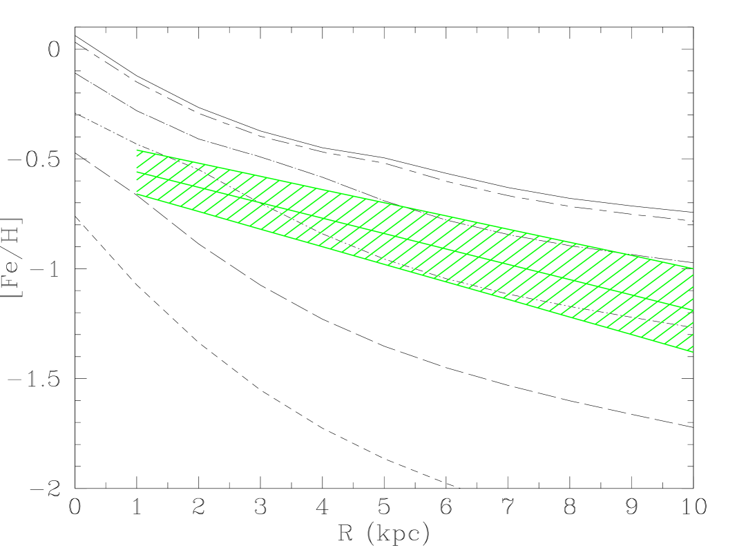
Figure 10: The time evolution of the [Fe/H] gradient according to our model (line types as in Fig.2), compared with the [Fe/H] gradient of RGB stars (Barker et al. barker06 (2006), shaded area).

4.4 Comparison with previous models

Specific models for the chemical evolution of M33 have been previously developed by Diaz & Tosi (diaz84 (1984)), Mollá et al. (molla96 (1996), molla97 (1997)), and by Mollá & Diaz (molla05 (2005)). Our approach is very similar to that of Mollá et al. (molla96 (1996), molla97 (1997)), and the predicted H I and H₂ radial distributions are indeed similar. The chemical gradients predicted by the model of Mollá et al. (molla96 (1996), molla97 (1997)) are however steeper (e.g. d(O/H)/dR $\sim$ -0.21 dex/kpc, d(N/H)/dR $\sim$ -0.34 dex/kpc) than what the most recent abundance determinations suggest. This is probably a consequence of the assumed IMF, heavily weighted towards massive stars in the parametrization adopted by Mollá et al. (molla96 (1996), molla97 (1997)). The time evolution of the metallicity gradients discussed in detail in Mollá et al. (molla97 (1997)), shows the same behaviour as in the present work, i.e. a flattening with time. Metallicity gradients resulting from the most recent models by Mollá & Diaz (molla05 (2005)), not computed specifically for M 33 but applied to the M 33 case, are also steeper than what the collection of observations presented here seem to show. Mollá & Diaz (molla05 (2005)) assume a slightly higher infall rate than Mollá et al. (molla96 (1996), molla97 (1997)), resulting in significantly higher surface density of H I and H₂, which are marginally consistent with the data. In particular their model predicts a strong decrease of the H I surface density towards the center, a large central H I hole, and a slight decrease of the H₂ surface density in the same region, which are not observed in this galaxy.

5 The time evolution of metallicity gradients

Both models we consider predict abundance gradients which flatten with time. The main difference between the two model is the resulting value of the slope of the gradients, that are much steeper at all times in the collapse model than in the accretion model. This is due to the different nature of the infall: the collapse model predicts a much shorter time scale for the formation of the disk, due to a rapid collapse of the halo, while the accretion model predicts a continuous infall of material from the intergalactic medium.

In the case of M33, the best fit to the whole set of observations is obtained with our accretion model, or, in the terminology by Mollá et al. molla93 (1993), with a model which has a self consistent SFR and a continuous gas infall. This model does not exclude an early collapse phase of a galactic halo, but considers its effects less important at the present time than the accumulation of matter from the intergalactic medium. This is supported by recent observations (see Sect. 2.4) and by numerical simulation of galaxy formation. As discusses in Sect. 3.1 the intergalactic supply is important, especially in low mass halos, and, in the case of M33. The continuous supply of gas is necessary to reproduce the high SFR observed at present time (see Fig. 2).

In Fig. 11 we compare the time evolution of the slope of the gradient of O/H and S/H (panel a, accretion model; panel b, collapse model) with the gradient measured in young stars, Hii regions and PNe. To derive the gradient, both the model predictions and the observational data have been linearly fitted in the $\log[M/H]$–$\log R$ plane, in the range of galactic radii 1–10 kpc. The flattening of the metallicity gradient predicted by the accretion model over the entire lifetime of the disk of M33 is quite modest because of the slow process of formation of the disk, which is still taking place at the present time. On the other hand, the collapse model predicts steeper gradients at all times, especially in the past, because of the rapid initial collapse phase that forms the disk in a few Gyr. This behaviour is in conflict with the observations, especially with the Fe/H gradient of RGB stars (see Sect. 4.3.5) determined by Barker et al (barker06 (2006)), as shown in Fig. 11c.

The comparison of the abundances in PNe with that in Hii regions presented in Sect. 4.3, represents the first evidence for a flattening of the abundance gradients with time in an external galaxy. A similar result has been found in the MW by Maciel et al. (maciel06 (2006)). The flattening in M33 is particularly evident for O and S abundances, as shown by Fig. 6 and Fig. 8. Another feature of particular interest in the case of M33 is the overall increase of metallicity with time at all radii. The steady infall rate, that increases the gas content of the disk with time, fuels star formation at all radii. The flattening of the gradient with time is due to the combination of the weak radial dependence of the infall rate and to the star formation efficiency which decreases more rapidly with time in the central regions.

Figure 11: The time evolution of the [O/H] (a), [S/H] (b), and [Fe/H](c) gradients according to our accretion (continuous line) and collapse (dotted line) models, compared with gradient slopes of sulfur (filled triangle) and oxygen (filled square) of PNe, of sulfur (empty triangle) and oxygen (empty square) of Hii regions and of young giant stars (star), and of iron of RGB stars (cross). The vertical dashed line marks the present age of the galaxy, 13.6 Gyr.

6 Conclusions

We have analyzed a large sample of observations for the LG spiral galaxy M33, including gas and stellar radial distributions, metallicity gradients, and star formation rate, and we have interpreted them using GCE models for this galaxy. We summarize here our main results:

• Our accretion model (where the infall rate on the disk is almost constant in time) reproduces the data better than our collapse model (where the accretion rate decreases rapidly to simulate the early collapse phase of a baryonic halo). Whereas both models can account (within the errors) for the observed distribution of stars, atomic and molecular gas, the abundance gradients, outlined by a large number of abundance determinations, and the high value of the present-day SFR allow one to discriminate between different accretion and SFR histories for this galaxy.

• The ability of our accretion model to reproduce the observed constraints suggests the existence of an extended phase for the formation of the disk of M33. The continuous accretion of material from the intergalactic medium, is also supported by deep observations at 21-cm in the proximity of M33 and by numerical simulation of galaxy formation and evolution. The continuous infall of gas into the disk is necessary to maintain a high SFR, declining very slowly with time.

• Chemical abundances determined in young stars, Hii regions, PNe, and RBG stars, all indicate a relatively flat radial distribution of elements, suggesting a slow, continuous rate of star formation in the disk of M33. The magnitude and evolution of the gradients of O/H, Ne/H, N/H, S/H, [Fe/H] computed with our accretion model are in good agreement with these observations. In particular, S/H and O/H gradients of PNe when compared with the same elemental abundance gradients of HII, and the [Fe/H] gradient of RGB stars, give independent observational evidence that the metallicity gradient has flattened over the last $\sim 8$ Gyr, in agreement with our model results. A similar behaviour has been recently found in the MW (Maciel et al. maciel06 (2006)) and may represent a general feature of the evolution of disk galaxies, even though galaxies of different masses, such as the MW and M33, might have followed different evolutionary histories.

Appendix A Chemical abundances in M33

We present here the collection of chemical abundance measurements used in the present work.

Table 4: Chemical abundances used to constrain the present chemical evolution model of M 33 from H II regions (S75, Smith smith75 (1975); KW81, Kwitter & Aller kwitter81 (1981); V88, Vilchez et al. vilchez88 (1988); C06, Crockett et al. crockett06 (2006); M07, Magrini et al. m07 (2007)), young stars (M97, Monteverde et al. monteverde97 (1997); U05, Urbaneja et al. urbaneja05 (2005); B06, Beaulieu et al. beaulieu06 (2006)), PNe (M04, Magrini et al. m04 (2004)). Chemical abundance marked with * are from recompilation by Garnett et al. (garnett97 (1997)) and those marked with : are derived without the electron temperature measurement. We adopted typical errors of 0.2 dex when they are not quoted.

Type	Name	RA	Dec	O/H	N/H	Ne/H	S/H	Ref.
		J2000.0
H II	BCLMP 93 (CC93)	1 33 52.3	+30 39 18	8.85*	-	-	-	S75 :
	BCLMP 87 (CC87)	1 34 01.0	+30 38 56	8.80*	-	-	-	S75 :
	NGC 595	1 33 35.50	+30 41 52.0	8.70*	-	-	-	S75 :
	NGC 604	1 34 33.19	+30 47 05.6	8.35*	7.30*	-	-	S75
	NGC 588	1 32 45.2	+30 38 54.0	8.45*	7.00*	-	-	S75
	IC 132	1 33 15.8	+30 56 45.0	8.05*	6.75*	-	-	S75
	BCLMP 85 (MA11)	1 34 07.0	+30 39 23	8.70*	7.35*	-	7.11	KW81 :
	IC 142	1 33 55.1	+30 45 22	8.72*	7.50*	7.42	6.78	KW81 :
	NGC 595	1 33 35.50	+30 41 52	8.22*	7.00*	7.75	7.01	KW81 :
	BCLMP 88 (MA 2)	1 34 15.5	+30 37 11	8.75*	7.50*	-	6.78	KW81 :
	MA 3	1 34 01	+30 52.1	8.45	7.10	7.63	6.75	KW81
	NGC 604	1 34 33.19	+30 47 05.6	8.30	6.97	7.49	6.70	KW81
	IC 131	1 33 15.0	+30 45 09	8.05	6.72	7.09	6.60	KW81
	BCLMP 650 (MA 9a)	1 34 33.64	+31 00 21.2	8.50*	7.2*	7.33	7.10	KW81 :
	IC 133	1 33 15.9	+30 53 02	8.25*	6.9*	7.55	6.95	KW81 :
	NGC 588	1 32 45.2	+30 38 54.0	8.00	6.84	7.30	6.68	KW81
	IC 132	1 33 15.8	+30 56 45.0	8.06	6.72	7.39	6.70	KW81
	BCLMP 93 (CC93)	1 33 52.3	+30 39 18	9.02$\pm$0.16	7.92	-	7.23$\pm$0.06	V88:
	IC 142	1 33 55.1	+30 45 22	8.70$\pm$0.16	7.57	-	7.03$\pm$0.05	V88
	NGC 595	1 33 35.50	+30 41 52	8.44$\pm$0.09	7.33	-	6.86$\pm$0.08	V88
	BCLMP 88 (MA 2)	1 34 15.5	+30 37 11	8.44$\pm$0.15	7.24	-	6.8$\pm$0.1	V88
	NGC 604	1 34 33.19	+30 47 05.6	8.51$\pm$0.03	7.35	-	6.95$\pm$0.03	V88
	IC 131	1 33 15.0	+30 45 09	8.41$\pm$0.06	7.25	-	-	V88
	NGC 588	1 32 45.2	+30 38 54.0	8.30$\pm$0.06	6.77	-	6.86$\pm$0.06	V88
	BCLMP 027	1 33 45.5	30 36 51	-	-	7.68$\pm$0.09	-	W03
	BCLMP 079	1 34 0.2	30 40 49	-	-	7.68$\pm$0.04	-	W03
	BCLMP 087E	1 34 2.5	30 38 41	-	-	7.96$\pm$0.08	-	W03
	BCLMP 042	1 33 5.5	30 39 30	-	-	7.89$\pm$0.10	-	W03
	BCLMP 301	1 33 5.3	30 45 22	-	-	7.63$\pm$0.08	-	W03
	BCLMP 004	1 33 9.3	30 35 49	-	-	7.85$\pm$0.08	-	W03
	BCLMP 062	1 33 4.5	30 44 38	-	-	7.55$\pm$0.08	-	W03
	BCLMP 049	1 33 3.9	30 41 28	-	-	7.77$\pm$0.04	-	W03
	BCLMP 045	1 33 8.8	30 40 25	-	-	7.66$\pm$0.04	-	W03
	BCLMP 302	1 34 6.9	30 47 26	-	-	8.00$\pm$0.04	-	W03
	BCLMP 214	1 33 30	30 31 47	-	-	7.84$\pm$0.08	-	W03
	BCLMP 095	1 34 0.9	30 36 18	-	-	7.87$\pm$0.08	-	W03
	BCLMP 088W	1 34 5.5	30 37 12	-	-	7.72$\pm$0.05	-	W03
	BCLMP 710	1 34 3.6	30 33 42	-	-	7.87$\pm$0.07	-	W03
	BCLMP 702	1 34 10	30 31 57	-	-	7.84$\pm$0.08	-	W03
	BCLMP 691	1 34 6.4	30 51 55	-	-	7.58$\pm$0.04	-	W03
	BCLMP 680C	1 34 2.1	30 47 0	-	-	7.70$\pm$0.03	-	W03
	BCLMP 680B	1 34 3.5	30 46 50	-	-	7.62$\pm$0.03	-	W03
	BCLMP 221	1 33 9.8	30 27 25	-	-	7.65$\pm$0.07	-	W03
	BCLMP 740W	1 34 9.6	30 41 52	-	-	7.46$\pm$0.05	-	W03
	CPDSP 194	1 33 1.1	30 45 16	-	-	7.53$\pm$0.07	-	W03
	BCLMP 251	1 3336.6	30 20 13	-	-	6.00$\pm$0.10	-	W03
	BCLMP 623	1 3316.5	30 52 50	-	-	6.90$\pm$0.03	-	W03
	BCLMP 280	1 3245.2	30 38 54	-	-	7.30$\pm$0.06	-	W03
	BCLMP 638E	1 3316.3	30 56 44	-	-	7.41$\pm$0.08	-	W03
	BCLMP 638N	1 3315.6	30 56 49	-	-	7.50$\pm$0.08	-	W03
	BCLMP 090	1 34 04.2	+30 38 09.2	8.50$\pm$0.06	-	7.96$\pm$0.09	-	C06
	BCLMP 691	1 34 16.6	+30 51 54.0	8.26$\pm$0.02	-	7.62$\pm$0.03	-	C06
	BCLMP 745	1 34 37.6	+30 34 55.0	8.07$\pm$0.10	-	7.2$\pm$0.2	-	C06
	BCLMP 706	1 34 42.2	+30 31 42.3	8.32$\pm$0.12	-	7.6$\pm$0.3	-	C06
	BCLMP 290	1 33 11.4	+30 45 15.1	8.21$\pm$0.06	-	7.4$\pm$0.1	-	C06
	MA1	1 33 03.4	+30 11 18.7	8.24$\pm$0.06	-	7.61$\pm$0.08	-	C06
	LGC HII 2	1 32 43.0	30 19 31.2	8.25 $\pm$0.06	7.17$\pm$0.25	-	6.75$\pm$0.18	M07
	LGC HII 3	1 32 45.9	30 41 35.5	8.24$\pm$0.05	6.94$\pm$0.17	-	6.62$\pm$0.11	M07
	BCLMP289	1 32 58.5	30 44 28.6	8.25$\pm$0.13	6.90$\pm$0.50	-	6.85$\pm$0.3	M07
	BCLMP218	1 33 00.3	30 30 47.3	8.25$\pm$0.05	7.19$\pm$0.14	-	6.77$\pm$0.15	M07
	MCM00Em24	1 33 10.8	30 18 08.5	8.18$\pm$0.25	7.10$\pm$0.30	-	6.55$\pm$0.3	M07
	CPSDP194	1 33 11.1	30 27 34.2	8.27$\pm$0.06	7.12$\pm$0.20	-	6.67$\pm$0.17	M07
	BCLMP626	1 33 16.4	30 54 04.8	8.13$\pm$0.07	6.86$\pm$0.30	-	6.61$\pm$0.28	M07
	BCLMP45	1 33 29.0	30 40 24.8	8.49$\pm$0.04	7.17$\pm$0.15	-	6.92$\pm$0.17	M07
	BCLMP637	1 33 50.6	30 56 33.3	8.34$\pm$0.05	7.30$\pm$0.40	-	6.90$\pm$0.40	M07
	GDK99 128	1 33 59.9	30 32 44.3	8.47$\pm$0.06	7.31$\pm$0.21	-	6.98$\pm$0.21	M07
	BCLMP670	1 34 03.3	30 53 09.3	8.28$\pm$0.07	7.14$\pm$0.30	-	6.75$\pm$0.18	M07
	VGHC 2-84	1 34 06.7	30 48 56.4	8.35$\pm$0.04	6.95$\pm$0.18	-	6.56$\pm$0.12	M07
	BCLMP717b	1 34 37.4	30 34 54.3	8.18$\pm$0.07	7.04$\pm$0.28	-	6.57$\pm$0.24	M07
	LGC HII 11	1 34 42.2	30 24 00.5	8.17$\pm$0.06	6.68$\pm$0.26	-	6.42$\pm$0.40	M07
giant stars	M33 1054	1 33 50.61	30 38 36.70	9.03	-	-	-	M97
	M33 1345	1 33 59.676	30 23 00.44	8.50	-	-	-	M97
	M33 B133	1 33 28.848	30 47 46.32	8.56	-	-	-	M97
	M33 110A	1 33 41.023	30 22 36.97	8.43	-	-	-	M97
	10900	1 33 44.90	+30 36 16.70	8.30$\pm$0.40	8.75$\pm$0.36	-	-	U05
	1110A	1 33 41.00	+30 22 37.00	8.40$\pm$0.40	8.50$\pm$0.42	-	-	U05
	1B38	1 33 00.83	+30 35 05.10	8.15$\pm$0.29	8.50$\pm$0.20	-	-	U05
	1B133	1 33 29.00	+30 47 44.00	8.10$\pm$0.16	8.30$\pm$0.17	-	-	U05
	11054	1 33 50.83	+30 38 34.50	8.10$\pm$0.15	8.90$\pm$0.18	-	-	U05
	11137	1 33 53.23	+30 35 26.10	8.50$\pm$0.30	8.70$\pm$0.25	-	-	U05
	1OB11241	1 33 42.02	+30 21 42.30	8.00$\pm$0.20	8.60$\pm$0.15	-	-	U05
	1UIT103	1 33 27.29	+31 00 56.70	7.90$\pm$0.10	8.20$\pm$0.13	-	-	U05
	1UIT122	1 33 33.70	+30 47 20.20	8.10$\pm$0.12	8.50$\pm$0.06	-	-	U05
	1UIT136	1 33 35.73	+31 00 47.00	7.70$\pm$0.19	8.40$\pm$0.18	-	-	U05
	1OB10-10	1 33 44.22	+30 31 48.20	8.55$\pm$0.21	8.65$\pm$0.22	-	-	U05
Cepheids	A121,029	1 34 59.72	30 52 25.2	8.22	-	-	-	B06
	B160,520	1 32 56.82	30 41 33.8	8.30	-	-	-	B06
	C133,449	1 34 33.43	30 51 15.6	8.56	-	-	-	B06
	D234,922	1 33 54.63	30 35 19.8	8.57	-	-	-	B06
	E237,367	1 34 03.97	30 38 08.4	8.58	-	-	-	B06
PNe	PN8	1 32 28.66	30 25 53.2	7.94	7.07	-	6.38	M04
	PN18	1 33 06.11	30 31 04.5	8.20	7.48	-	6.83	M04
	PN28	1 33 19.25	30 29 40.4	8.69	6.98	-	6.47	M04
	PN60	1 33 46.42	30 26 55.3	8.69	7.67	-	6.57	M04
	PN65	1 33 49.37	30 32 06.3	8.67	7.61	-	6.84	M04
	PN75	1 34 01.14	30 50 27.1	8.49	8.03	-	6.81	M04
	PN91	1 34 13.97	30 22 36.4	8.48	8.07	-	6.60	M04
	PN93	1 34 15.88	30 24 54.6	8.47	7.75	-	6.66	M04
	PN96	1 34 15.44	30 32 20.2	8.76	7.43	-	6.44	M04
	PN101	1 34 24.25	30 27 54.3	8.72	7.33	-	6.18	M04
	PN125	1 34 32.85	30 41 10.5	8.31	7.53	-	6.66	M04

Table 4: continued.