The Ionization Fraction of Barnard 68: Implications for Star and Planet Formation

Abstract

We present a detailed study of the ionization fraction of the Barnard 68 pre-stellar core, using millimeter $\mathrm{H^{13}CO^{+}}$ and $\mathrm{DCO^{+}}$ lines observations. These observations are compared to the predictions of a radiative transfer model coupled to a chemical network that includes depletion on grains and gas phase deuterium fractionation. Together with previous observations and modelling of CO and isotopologues, our $\mathrm{H^{13}CO^{+}}$ and $\mathrm{DCO^{+}}$ observations and modelling allow to place constraints on the metal abundance and the cosmic ionization rate. The $\mathrm{H^{13}CO^{+}}$ emission is well reproduced for metals abundances lower than $3\times 10^{-9}$ and a standard cosmic ray ionization rate. However, the observations are also consistent with a complete depletion of metals, i.e. with cosmic rays as the only source of ionization at visual extinctions greater than a few $A_{v}$. The $\mathrm{DCO^{+}}$ emission is found to be dependent of the ortho to para H₂ ratio, and indicates a ratio of $\sim 10^{-2}$. The derived ionization fraction is about $5\times 10^{-9}$ with respect to H nuclei, which is about an order of magnitude lower than the one observed in the L1544 core. The corresponding ambipolar diffusion timescale is found to be an order of magnitude larger than the free fall timescale at the center of the core. The inferred metal abundance suggests that magnetically inactive regions (dead zones) are present in protostellar disks.

1 Introduction

The ionization fraction (or the electron abundance) plays an important role in the chemistry and the dynamics of prestellar cores. Because of the low temperature, the chemistry is dominated by ion neutral reactions (Herbst & Klemperer, 1973), and electronic recombination is one of the major destruction pathways for molecular ions. Furthermore, the ionization fraction sets the coupling of the gas with the magnetic field (Shu et al., 1987).

Several attempts have been made to estimate the electron fraction in dense clouds and prestellar cores (Guélin et al., 1982; Wootten et al., 1982; de Boisanger et al., 1996; Williams et al., 1998; Caselli et al., 1998). These studies rely on measurements of the degree of deuterium fractionation (though the $\mathrm{DCO^{+}}$ over $\mathrm{HCO^{+}}$ abundance ratio for example), which has been found to be roughly inversely proportional to the electron abundance (Langer, 1985). However, this simple approach has caveats (Caselli, 2002) as it does not consider line-of-sight variations of the electron fraction. Large density gradients exist in prestellar cores, and therefore one may anticipate similar variations in the electron abundance. In addition, the freeze-out of molecules onto the grain surfaces (e.g.  Tafalla et al., 2002; Bergin et al., 2002) influence the degree of deuterium fractionation independently of the electron fraction (Caselli et al., 1998). Finally, these studies usually consider simple chemical networks that may neglect important ingredients for the electron fraction.

In this paper, we study the ionization fraction in the Barnard 68 core, using $\mathrm{H^{13}CO^{+}}$ and $\mathrm{DCO^{+}}$ line observations. These observations are interpreted with a chemical network including gas-grain interactions that is coupled to a radiative transfer model. This technique allows us to infer the electron abundance along the line-of-sight, and to place constraints on the abundance of metals, the cosmic ray ionization rate, and the ionization state of material that is provided by infall to the forming proto-planetary disk.

The paper is organized as follows: in Section 2, we present the observations. The model used to interpret these observations is detailed in Section 3. Implications of our findings are discussed in Section 5, and Section 6 concludes this paper.

2 Observations

The H¹³CO⁺ (1-0) ($\nu=86.754288$ GHz), and the DCO⁺ (2-1) ($\nu=144.077319$ GHz) transitions were observed towards B68 ($\alpha=17^{\mathrm{h}}22^{\mathrm{m}}38.2^{\mathrm{s}}$ and $\delta=-23\arcdeg 49\arcmin 34.0\arcsec$; J2000) in April 2002 and September 2002 using the IRAM-30m telescope. The core was mapped with a spatial sampling of 12″. The half power beam size of the telescope is $29\arcsec$ at 87 GHz and $17\arcsec$ at 144 GHz. System temperature were typically $\sim 110-150$ K at 3 mm and $\sim 160-350$ K at 2 mm. Pointing was regularly checked using planets and was found to be better than $\sim 2\arcsec$. The data were calibrated in antenna temperature ($T_{\mathrm{a}}^{*}$) units using the chopper wheel method, and were converted to the main beam temperature scale ($T_{\mathrm{mb}}$), using the telescope efficiencies from the IRAM website. All observations were carried out in frequency switching mode. The H¹³CO⁺ (1-0) data were also presented in Maret et al. (2006).

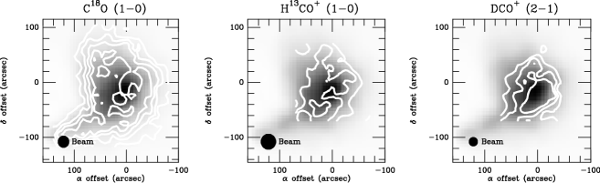
Figure 1: Comparison between integrated intensity maps (contours) of C¹⁸O (1-0) (left, from Bergin et al. 2002), H¹³CO⁺ (1-0) (center) and DCO⁺ (2-1) (right) superposed on the map of visual extinction obtained by Alves et al. (2001). C¹⁸O (1-0) contours start at 0.2 K km s^-1 and step by 0.2 K km s^-1. H¹³O (1-0) contours start at 0.15 K km s^-1 and step by 0.15 K km s^-1. DCO⁺ (1-0) contours start at 0.1 K km s^-1 and step by 0.1 K km s^-1. The $A_{V}$ image range from 0 to 27 mag.

Fig. 1 shows a comparison between the integrated line intensity maps of DCO⁺ (2-1) and H¹³CO⁺ (1-0) with the visual extinction map obtained by Alves et al. (2001). The C¹⁸O (1-0) map from Bergin et al. (2002) is also shown. On this figure, we see that the peak of H¹³CO⁺ (1-0) line emission does not correspond to the maximum visual extinction in the core. The C¹⁸O (1-0) line emission shows a similar behavior: it peaks in a shell-like structure with a radius of $\sim 50\arcsec$ around the maximum visual extinction. The DCO⁺ (2-1) line emission, on the other hand, seems to correlate well with the visual extinction. These differences are likely a consequence of chemical effects. Because of the freeze-out on grain mantles, the abundance of CO and its isotopologues decrease by about two orders of magnitude towards the center of the core (Bergin et al., 2002). Since H¹³CO⁺ is mainly formed from the reaction of ¹³CO with H${}_{3}^{+}$, its abundance is also expected to decrease towards the core center. DCO⁺ should also be affected by the depletion of CO. However, the deuterium fractionation increases as CO is removed from the gas phase. Thus the disappearance of CO might be compensated by the increased deuterium fractionation. In the following, we interpret the emission of these species using a chemical model coupled with Monte-Carlo radiative transfer model, in order to derive precisely their abundance profiles.

3 Analysis

We have used a technique that combines the predictions of a chemical network with a Monte-Carlo radiative transfer (Bergin et al., 2002, 2006; Maret et al., 2006). The outline of this technique is the following. Chemical abundances are computed as a function of the visual extinction in the core. Using these abundance profiles, the line emission is computed with a Monte Carlo radiative transfer code. The resulting map is convolved to the resolution of the telescope, and is compared to the observations. Free parameters of the chemical model (e.g. cosmic ionization rate, metal abundances, etc.) are adjusted until a good agreement is obtained between the model and the observations. Thus, this technique allows for a direct comparison between the predictions of the chemical network and the observations.

We have used the chemical network of Bergin et al. (1995). This network is contains about 150 species (including isotopologues, see below), and focuses on the formation of simple molecules and ions (e.g. CO and HCO⁺). The network includes the effect of depletion on grains, and the desorption by thermal evaporation, UV photons, and cosmic rays (Hasegawa & Herbst, 1993; Bringa & Johnson, 2004). It also includes the effect of fractionation of ¹³C and ¹⁸O, using the formalism described by Langer & Penzias (1993). We have extended this network to include the effect of deuterium fractionation, following the approach used by Millar et al. (1989). Because of the importance of multiply deuterated species in the deuterium fractionation process, these species were also included in the network, following Roberts et al. (2004). It also include neutralization reactions of ions on negatively charged grains. The predictions of our network were checked against the UMIST network (Millar et al., 1997) for consistency.

We adopt the density profile determined by Alves et al. (2001), from observations of near infrared extinction from background stars. This profile is assumed to be constant as a function of time. The dust temperature profile was computed using the analytical formulae from Zucconi et al. (2001). For the gas temperature we have adopted the profile determined by Bergin et al. (2006) from observations and modelling of CO and its isotopologues. The gas temperature is relatively low (7-8 K), and increases sightly (10-11 K) at the center of the core as indicated by ammonia lines observations (Lai et al., 2003). This increase in the temperature is a result of grain coagulation at the center of the core, which produces a thermal decoupling between the gas and the cooler dust.

The cloud is supposed to have the initial composition summarized in Table 1. In our model, we assume that the density profile of the core does not evolve with time. Therefore, we also assume that the chemistry has already evolved to a point where hydrogen is fully molecular, and all the carbon is locked into CO. Our treatment of the initial atomic oxygen pool deserves special mention. Bergin & Snell (2002) examined this question in the context of the non-detection of water vapor emission in B68 by SWAS. They found that if atomic oxygen were present in the gas phase in the dense core center, then the well studied reaction chain that forms $\mathrm{H_{2}O}$ (via $\mathrm{H_{3}O^{+}}$) would have yielded detectable water vapor emission. The simplest way to stop this reaction chain is to remove the fuel for the gas-phase chemistry: atomic oxygen. This happens when oxygen is trapped on grain surfaces in the form of water ice (e.g.  Bergin et al., 2000). Thus we have assumed initial conditions in which all non-refractory oxygen is in the form of water ice and CO gas with no atomic oxygen left. In this fashion our initial abundances assume the core formed out of gas that reached at $A_{v}\sim 2$ – where $\mathrm{H_{2}}$ and CO have formed and water ice mantles are observed. On the other hand, nitrogen is assumed to be mostly in atomic form (Maret et al., 2006).

A grain size of 0.1 $\mu m$ is assumed. The cosmic ray ionization rate and the abundance of low ionization potentials metals ($<$ 13.6 eV) are free parameters of our study (see §4.1 and §4.2). In our models we combine all metals (e.g. Fe⁺, Mg⁺, …) into one species, labeled as M⁺ with the Fe⁺ recombination rate of $\alpha(\mathrm{M}^{+})=3.7\times 10^{-12}(T/300\,\mathrm{K})^{-0.65}\,\mathrm{cm^{3}\,s^{-1}}$. Due the low ionization potential these metals are assumed to be fully ionized at the start of the calculation. The network also includes the neutralization of ions of negatively charged grains with one electron per grain.

The core is assumed to be bathed in a UV field of 0.2 (in Habing units; 1968), as determined by Bergin et al. (2006). The chemical abundances are computed as a function of time by solving the rate equations using the DVODE algorithm (Brown et al., 1989). This is done until a time of $10^{5}\ \mathrm{yr}$ is reached. This corresponds to the “best-fit” model of Bergin et al. (2006). However, as discussed by Bergin et al., this time is a lower limit of the real age of the cloud, since the CO is assumed to be pre-existing at $t=0$ in these models.

Modeling the line emission requires the knowledge of velocity profile in the core. As a first approach, we have neglected systematic motions (see Lada et al., 2003; Redman et al., 2006), and we have used the turbulent velocity profile determined by Bergin et al. (2006) from $\mathrm{C^{18}O}$ and $\mathrm{{}^{13}CO}$ lines. The turbulent velocity is $\sim 0.3$ km/s at the edge of the cloud, and decreases significantly ($\sim 0.15$ km/s) towards the center of the core.

4 Results

4.1 Metals depletion

Metals ions (e.g. Fe⁺ and Mg⁺) play an important role in in setting the electron abundance in pre-stellar cores, because they are destroyed relatively slowly by radiative recombination. For example, the recombination rate of H${}_{3}^{+}$ is four order of magnitude higher than the rate for Fe⁺.

Guélin et al. (1982) measured the electron abundance in a sample of dense molecular clouds using HCO⁺ and DCO⁺ line observations, and obtained values comprised between 10^-8 and 10^-7. The authors concluded that the metal abundance is lower than 10^-7 in these clouds. Caselli et al. (1998) determined the electron abundance in a sample of twenty four low-mass isolated cores (with embedded stars and starless – similar in properties to B68) from CO, HCO⁺ and DCO⁺ observations, and obtained values in the range 10^-8-10^-6. Caselli et al. argued that the differences between cores are due to changes in metal abundance and a variable cosmic ionization rate ($\zeta$). The best fit between their chemical model predictions and the observations indicates metal abundances in the range $2\times 10^{-9}-3\times 10^{-7}$. Williams et al. (1998) determined the electron abundance in a similar sample of low mass cores using a slightly different approach, and obtained metal abundances comprised between $5\times 10^{-9}$ and $4\times 10^{-8}$ (assuming a constant $\zeta$). All these studies indicate low metal abundances with respect to their solar values.. Indeed, observations of FUV FeII absorption lines, and other metal lines, towards diffuse clouds find depletion factors of over two order of magnitude with respect to solar values (Savage & Bohlin, 1979; Jenkins et al., 1986; Snow et al., 2002).

Our $\mathrm{H^{13}CO^{+}}\ (1-0)$ observations can be used to set limits on the metal ion abundance in B68. $\mathrm{H^{13}CO^{+}}$ is sensitive to the electron abundance inside the core, because it is mainly destroyed by electronic recombination. It is also sensitive to the $\mathrm{H_{3}^{+}}$ and $\mathrm{{}^{13}CO}$ abundances, since it is formed from the reaction between these two species. $\mathrm{H_{3}^{+}}$ itself is mainly formed from $\mathrm{H_{2}}$ ionization by cosmic rays. The remaining parameter in determining the chemical abundance profile is the time dependence of the chemistry. In this case, our analysis is simplified because Bergin et al. (2006) used multiple transitions of ¹³CO and C¹⁸O and a similar modeling technique to derive the ¹³CO abundance and constrain the “chemical age” of Barnard 68 to $t=10^{5}\,\mathrm{yr}$. Thus, the only free parameters for our modeling of the $\mathrm{H^{13}CO^{+}}$ emission are the cosmic ionization rate $\zeta$ and the metal ion abundance. These two parameters are difficult to constrain simultaneously. In Maret et al. (2006), we found that the $\mathrm{H^{13}CO^{+}}\ (1-0)$ line emission in B68 is well reproduced by our chemical network if one assume a metal abundance of $3\times 10^{-9}$ with respect to H nuclei and a standard cosmic ionization rate ($\zeta=3\times 10^{-17}\ \rm{s}^{-1}$, see next section). In the following, we explore the parameter space into more details to place constrains on the metal abundance in the core.

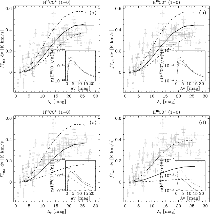
Figure 2: Comparison between the observations and the model predictions of the $\mathrm{H^{13}CO^{+}}$ (1-0) line for different cosmic ionization rates ($\zeta$) and metal abundances. Blue points with error bars (1 $\sigma$) represent the observed integrated line intensity as a function of the visual extinction in the core ($A_{v}$). Dashed, solid and dash-dotted lines represent the model predictions for $\zeta=3\times 10^{-18}$, $3\times 10^{-17}$ and $3\times 10^{-16}\,\mathrm{s^{-1}}$ respectively. In panel (a) a complete depletion of metals is assumed. In panels (b), (c), and (d), a metals abundance of respectively $3\times 10^{-10}$, $3\times 10^{-9}$ and $3\times 10^{-8}$ is assumed.

On Fig. 2, we show the predicted intensity of the $\mathrm{H^{13}CO^{+}}$ (1-0) line for different metal ion abundances and cosmic ionization rates. In these models, metals are assumed to be initially fully ionized. In Fig. 2, we see that for $\zeta=3\times 10^{-17}\ \rm{s}^{-1}$, our model predicts the same intensities for $x(\mathrm{M}^{+})$ = 0 and $x(\mathrm{M}^{+})=3\times 10^{-10}$. The predicted emission is in fairly good agreement with the observations. On the other hand, for a higher metal abundance ($x(\mathrm{M}^{+})=3\times 10^{-9}$) the model predicts a intensity slightly lower than the observed, but is in better agreement with the observations at the center of the core. A metal abundance of $3\times 10^{-8}$ is clearly ruled out by the model and observation comparison. We conclude that $x(\mathrm{M}^{+})\leq 3\times 10^{-9}$. This value is at the low end of the one obtained by Caselli et al. (1998) and Williams et al. (1998). Compared to the abundance of metals in the solar photosphere ($x(\mathrm{M})\sim 8.5\times 10^{-5}$; Anders & Grevesse, 1989), this represent a depletion factor of more than four orders of magnitude. Indeed, our observations are also fully consistent with a complete depletion of metals in the core, i.e. with cosmic rays as the only source of ionization at $A_{v}$ greater than a few magnitudes (see Fig. 2). It should be noted, however, that result depends on the value of $\zeta$ adopted. For example, our observations are fully consistent with a cosmic ionization rate of $3\times 10^{-16}\ \rm{s}^{-1}$ and $x(\mathrm{M}^{+})=3\times 10^{-8}$. The effects of varying $\zeta$ are discussed in the next section.

4.2 Cosmic Ray Ionization Rate

Cosmic rays play a crucial role in the chemistry of pre-stellar cores, because they set the abundance of the pivotal H${}_{3}^{+}$ ion, and are the only source of ionization at $A_{v}$ greater than a few magnitudes. Despite of its importance, the cosmic ray ionization rate is difficult to constrain (see Le Petit et al. 2004, van der Tak et al. 2006 and Dalgarno 2006 for recent reviews). Early estimates in diffuse clouds from HD and OD observations indicate $\zeta=7\times 10^{-17}\,\mathrm{s}^{-1}$ (van Dishoeck & Black, 1986), a value in agreement with the lower limit of $3\times 10^{-17}\,\mathrm{s}^{-1}$ measured by the Voyager and Pioneer satellites (Webber, 1998). $\mathrm{H_{3}^{+}}$ observations towards $\zeta$ Persei cloud suggest a significantly higher rate ($\zeta=1.2\times 10^{-15}\,\mathrm{s}^{-1}$; McCall et al., 2003). However, Le Petit et al. (2004) argued that a value of $\zeta=2.5\times 10^{-16}\,\mathrm{s}^{-1}$ is more consistent with both $\mathrm{H_{3}^{+}}$ and HD observations. In denser regions, $\mathrm{HCO^{+}}$ observations indicates a lower ionization rate than in diffuse clouds: van der Tak & van Dishoeck (2000) obtained $\zeta=(2.6\pm 1.8)\times 10^{-17}\,\mathrm{s}^{-1}$ from $\mathrm{HCO^{+}}$ line observations towards massive protostars. In pre-stellar cores, Caselli et al. (1998) inferred a value comprised between $10^{-18}$ and $10^{-16}\,\mathrm{s}^{-1}$. The difference in the cosmic ray ionization rate between diffuse and dense clouds could be due to the scattering of cosmic rays (Padoan & Scalo, 2005). In addition, large variations are inferred as a function of the Galactic Center distance (Oka et al., 2005; van der Tak et al., 2006).

Cosmic rays are also heating agents of the gas. Bergin et al. (2006) examined the value of $\zeta$ in B68 by comparing the predictions of a chemical and thermal model to observations of CO and its isotopologues. Bergin et al. found that their model provide reasonable fits to the data for $\zeta=1-6\times 10^{-17}\ \mathrm{s}^{-1}$. Their “best fit” model has $\zeta=1.5-3\times 10^{-17}\ \mathrm{s}^{-1}$. Here we examine the constraints placed by our $\mathrm{H^{13}CO^{+}}$ observations. On Fig. 2, we see that our model produces a good fit to the data for $\zeta=3\times 10^{-17}\ \mathrm{s}^{-1}$, except for $x(\mathrm{M}^{+})=3\times 10^{-8}$, where the model predictions underestimate the observation by a factor two. Models with $\zeta=3\times 10^{-18}\ \mathrm{s}^{-1}$, consistently underestimate the observations. Conversely models with $\zeta=3\times 10^{-16}\ \mathrm{s}^{-1}$ overestimate the model, except the one with $x(\mathrm{M}^{+})\leq 3\times 10^{-8}$. This in agreement with Bergin et al. (2006), who found that their observations are not reproduced by models with $\zeta=6\times 10^{-16}\ \mathrm{s}^{-1}$.

To summarize our conclusions regarding the metals abundances and the cosmic ionization rate, models with $x(\mathrm{M}^{+})\leq 3\times 10^{-9}$ provide a good agreement with the data, although the model with $x(\mathrm{M}^{+})=3\times 10^{-8}$ and $\zeta=3\times 10^{-16}\ \mathrm{s}^{-1}$ is also consistent with our data. However values of $\zeta$ greater that $6\times 10^{-17}{s}^{-1}$ are ruled out by Bergin et al. (2006) based on core thermal balance. On the other hand, models with $\zeta=3\times 10^{-18}\ \mathrm{s}^{-1}$ always underestimate our observations. We conclude that $\zeta=1-6\times 10^{-17}\ \mathrm{s}^{-1}$, and $x(\mathrm{M}^{+})\leq 3\times 10^{-9}$ in B68. This implies that the abundance of ionized metals is reduced in the center of B68. Charge transfer from molecular ions (e.g. H${}_{3}^{+}$, HCO⁺) to metals can be important and a reduction in the abundance of ionized metals also requires lowering the neutral metal abundance. In the case of Fe a potential reservoir is FeS (Keller et al., 2002), or organometallic molecules (Serra et al., 1992). An other possility is that Fe is incorporated into grain cores.

4.3 Ortho to para H₂ ratio

The ortho to para H₂ ratio influences the degree of ion and molecule deuteration in prestellar cores (Pineau des Forets et al., 1991; Flower et al., 2006b). In the gas phase, deuterium fractionation is mainly due to the following reaction (see Roberts et al., 2004, and references therein):

$$\mathrm{H_{3}^{+}+HD\rightleftharpoons H_{2}D^{+}+H_{2}}$$ (1)

The reverse reaction has an activation barrier of $\sim 232\ \mathrm{K}$ and therefore the reaction becomes essentially irreversible at low temperature. Gerlich et al. (2002) measured the forward and reverse rates of the above reaction at 10 K, and found them to be very different than commonly adopted values. The forward reaction rate was found to be about five times higher than previous estimates (Sidhu et al., 1992), while the reverse reaction rate was found to be five orders of magnitude larger than previously used (e.g.  Caselli et al., 1998). In addition, Gerlich et al. (2002) determined via a laboratory measurement that the reverse reaction rate is very sensitive to the ratio of ortho to para molecular hydrogen. This is because o-H₂, in its ground rotational level ($J=1$) has an higher energy ($\Delta E\sim 170.5\ \mathrm{K}$) when compared to the ground state of p-H₂ ($J=0$). Consequently, o-H₂ can more easily cross the energy barrier than p-H₂, and the rate of the reverse reaction increases with the ortho to para H₂ ratio.

Our $\mathrm{DCO^{+}}$ observations can be used to estimate the $\mathrm{H_{2}D^{+}}$ abundance, and thus the efficiency of the deuterium fractionation process. $\mathrm{DCO^{+}}$ is mainly formed by the following reaction:

$$\mathrm{H_{2}D^{+}+CO\rightarrow DCO^{+}+H_{2}}$$ (2)

and is mainly destroyed by electronic recombination. Thus the $\mathrm{DCO^{+}}$ emission depends on both the CO and $\mathrm{H_{2}D^{+}}$ abundances, the electron fraction (induced by cosmic-rays and by pre-existing metal ions), the ortho to para H₂ ratio, and on time. Here we benefit from our previous analysis of CO which constrained the CO abundance and “chemical age” and our analysis of $\mathrm{H^{13}CO^{+}}$ which limit the metal ion abundance and cosmic ray ionization rate. Thus the primary free parameter is the ortho to para $\mathrm{H_{2}}$ ratio ($o/p$) when we adopt our best fit parameters of $x(M^{+})=3\times 10^{-9}$ and $\zeta=3\times 10^{-17}\,\mathrm{s^{-1}}$.

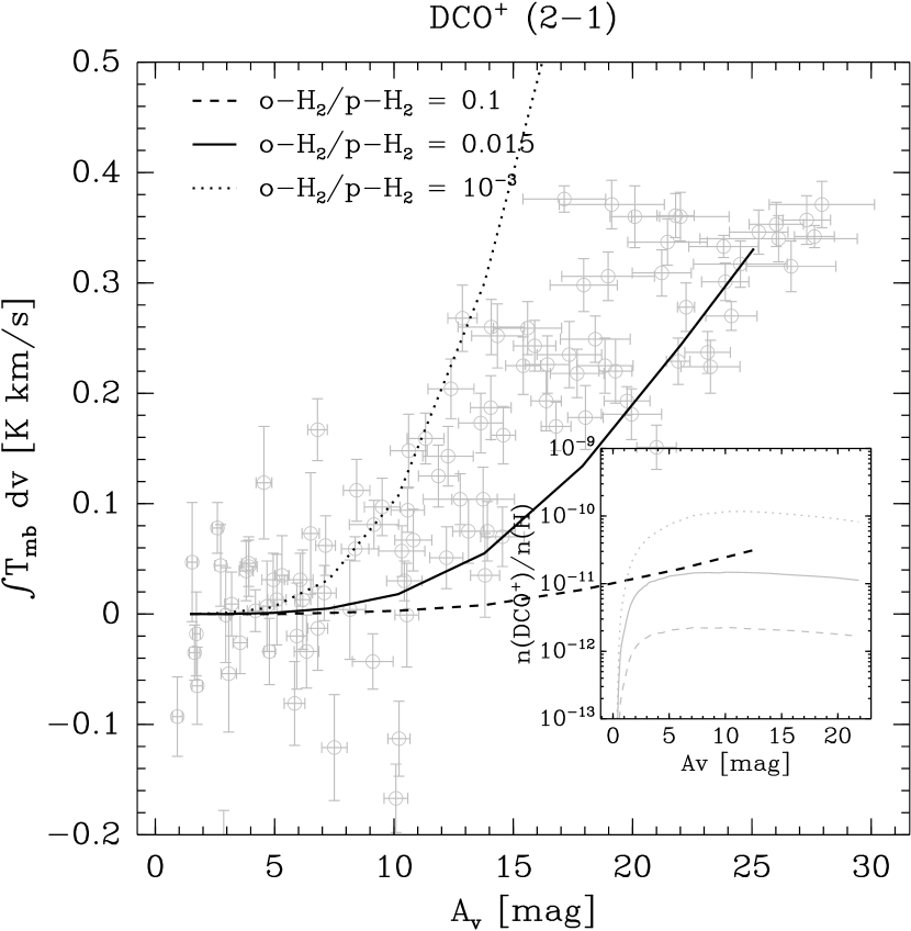
Figure 3: Comparison between the observations and the model predictions of the $\mathrm{DCO^{+}}$ (2-1) line for different ortho to para $\mathrm{H_{2}}$ ratios. Blue points with error bars (1 $\sigma$) represent the observed integrated line intensity as a function of the visual extinction in the core ($A_{v}$). The dashed, dotted and solid black lines show the predicted line intensity for different ortho to para $\mathrm{H_{2}}$ ratios. The inset show the corresponding abundances of $\mathrm{DCO^{+}}$.

On Fig. 3, we compare the observed $\mathrm{DCO^{+}}$ (1-0) line emission as a function of $A_{v}$, with the predictions of our model for different ortho to para H₂ ratio. Note that in these models, no $o/p$ conversion is considered: the ortho to para H₂ ratio is assumed to be constant. The best agreement between the observations and the model is obtained for an $o/p$ ratio of $\sim 1.5\times 10^{-2}$, well above the Boltzmann equilibrium value at 10 K ($3.5\times 10^{-7}$). Fig. 3 also show the derived $\mathrm{DCO^{+}}$ abundance inside the core. The abundance peaks at an $A_{v}$ of $\sim 5$, and decreases slightly towards the core center, as a consequence of CO depletion (see Section 5.1).

It is interesting to compare the $o/p$ H₂ ratio we obtain with the predictions of other models. Walmsley et al. (2004) modeled the $o/p$ H₂ ratio in prestellar cores, assuming a complete depletion of heavy elements. In their model, an initial o/p H₂ ratio of $3.5\times 10^{-7}$ is assumed. For a density of $10^{6}\ \mathrm{cm}^{-3}$, steady-state is reached in $10^{5}$ yr, a time comparable to the age of B68 inferred from CO depletion observation and modeling (Bergin et al., 2006). At steady state, the o/p H₂ ratio obtained is $6\times 10^{-5}$, i.e. about two orders of magnitude lower than the value determined in this work. However, as noted by Flower et al. (2006a), the ortho to para H₂ ratio conversion reactions are very slow, and it is not clear if the steady state equilibrium is reached in molecular clouds prior to the formation of dense cores. Using a initial ortho to para ratio of 3 (a value appropriate for H₂ formation on grains), Flower et al. (2006b) obtain a steady state ratio of $3\times 10^{-3}$. This value, although still about a factor 5 lower, is in better agreement with our estimate. We note that for $o/p=3\times 10^{-3}$, our model predicts an DCO⁺ (1-0) emission about 2 times higher than the observations (see Fig. 3).

5 Discussion

5.1 Electron abundance and main charge carriers

On Fig. 4, we show the derived electron and main ions abundances inside the core. The electron abundance is $\sim 5\times 10^{-9}$ with respect to H nuclei throughout most part of the core. At low $A_{v}$, the electron abundance increases as a result of photo-dissociation of CO. In this region, the most abundant ion is C⁺. At higher $A_{v}$, the most abundant ion is H${}_{3}^{+}$, which caries about $\sim 20\%$ of the electric charge. The remainder of the charge is shared between more complex ions. Deuterated ions do not contribute significantly to the ionization fraction. In the innermost region of the core, where the deuteration increases as a result of CO depletion, the main deuterated ion, D${}_{3}^{+}$, is about ten times less abundant than H${}_{3}^{+}$. H₂D⁺ and D₂H⁺ have similar abundances ($2\times 10^{-11}$ with respect to H). This is in agreement with recent observations (Vastel et al., 2004).

Recently, Hogerheijde et al. (2006) reported a probable detection of $\mathrm{o-H_{2}D^{+}}$ fundamental line towards B68 which can be compared to our model predictions. The measured flux is however quite uncertain, given the relatively low signal to noise ratio of this observation (2.7$\sigma$ and 5.2$\sigma$ on the peak and integrated intensity, respectively). Assuming a thermal excitation (10 K) and optically thin conditions, Hogerheijde et al. derive a $\mathrm{H_{2}D^{+}}$ column density of $1.5\times 10^{12}$ cm^-2. Assuming a H₂ column density of $3.6\times 10^{22}$ cm^-2 (Alves et al., 2001), this corresponds to an $\mathrm{H_{2}D^{+}}$ abundance of $2.1\times 10^{-11}$ with respect to H nuclei, averaged in the APEX beam (17″), with respect to H nuclei. This is in excellent agreement with our model, which predicts an H₂D⁺ abundance of $2\times 10^{-11}$, roughly constant across the envelope. Of course, if the excitation is non-thermal, the detection implies an higher abundance. Assuming a 5 K excitation temperature, Hogerheijde et al. derive a beam averaged abundance of $1.5\times 10^{-10}$ with respect to H nuclei. This is about an order of magnitude higher than our model predictions. Since no collisional rates exist in the literature for $\mathrm{H_{2}D^{+}}$, it is unclear whether or not the excitation of this line is thermal. Hogerheijde et al. estimate a critical density of $2\times 10^{6}$ cm^-3, which exceeds the density at the center of B68 ($3\times 10^{5}$ cm^-3) by about an order of magnitude. However, the collisional rate, and therefore the critical density, is uncertain by an order of magnitude (van der Tak et al., 2005; Hogerheijde et al., 2006). Our model predictions regarding the deuterium chemistry could be also tested via observations of the $\mathrm{D_{2}H^{+}}\ 1_{1,0}-1_{0,1}$ ($\nu$ = 691.66044 GHz). Assuming a excitation temperature of 10 K, we predict a line intensity of 10 mK. Unfortunately, this is too weak to be detected with current ground based telescopes.

We would like to compare the electron abundance profile we obtained with the one derived by Caselli et al. (2002) in L1544. In the Caselli et al. best fit model, the electron abundance at the center of L1544 is $5\times 10^{-10}$ (with respect to H), while we obtain an electron abundance an order of magnitude higher at the center of B68. These differences are probably a consequence of different central densities: the L1544 central density is about an order of magnitude higher than the one of B68, and the electron fraction is expected to scale as $n(\mathrm{H}_{2})^{-1/2}$ (McKee, 1989). Another important difference is the dominant ion: Caselli et al. (2002) predicts that the most abundant ion is $\mathrm{H_{3}O^{+}}$, while in our modeling main charge carrier is $\mathrm{H_{3}^{+}}$. These differences are due to different assumptions on the atomic oxygen abundance. Caselli et al. (2002) assumes that oxygen is initially mostly atomic. As a consequence, the $\mathrm{H_{3}O^{+}}$ abundance is relatively large, because atomic oxygen reacts with $\mathrm{H_{3}^{+}}$ to form $\mathrm{H_{3}O^{+}}$ (after successive protonations by H₂ followed by recombination). In our modeling, oxygen is assumed to be initially locked in water ices and gas phase CO (see Table 1), and the atomic oxygen gas phase abundance is relatively low.

Finally, we would like to comment on the effect of grain size evolution on the electron fraction in the core. Walmsley et al. (2004) computed the electron abundance and main charge carrier in a prestellar core for different grain sizes. For a grain size of 0.02 $\mu m$, the main charge carrier in their model is H${}_{3}^{+}$, while for larger grains (0.1 $\mu m$), the most abundant ion becomes H⁺. In their models, H⁺ recombines primarily on grains, while H${}_{3}^{+}$ recombines with free electrons. Since the recombination timescale on grains depends on the grain size, the H⁺ over H${}_{3}^{+}$ abundance ratio, and in turn the electron abundance, depends on the grain size as well. However, these models assume a complete depletion of heavy elements, which is not the case for B68. In B68 we do find evidence for strong molecular, but not complete, heavy element freeze-out, at the core center. The reaction with H⁺ with molecules containing these elements (e.g. NH₃, OH, …) can transfer the charge to molecular ions with faster recombination timescales. This would probably reduce the dependence of the electron abundance on the grain size.

5.2 Core stability

The electron abundance in the core is also important for its dynamical evolution, since its affects the efficiency of ambipolar diffusion. In a weakly ionized sub-critical core, the ions are supported against collapse by the magnetic field, but neutrals can slowly drift with respect to the ions (see Shu et al., 1987, for a review). The timescale for this phenomenon is given by Walmsley et al. (2004):

$$\tau_{\mathrm{ad}}=\frac{2}{\pi Gm_{n}^{2}}\sum_{i}\frac{n_{i}}{n_{n}}\frac{m_{i}m_{n}}{m_{i}+m_{n}}\langle\sigma v\rangle_{in}$$ (3)

where G is the gravitational constant, m_n and m_i are the masses of the neutrals and the ions respectively, n_n and n_i are the number densities, $\langle\sigma v\rangle_{in}$ is the rate coefficient for the momentum transfer, and the summation goes over all ions. At low temperature, the rate coefficient for momentum transfer is (Flower, 2000):

$$\langle\sigma v\rangle_{in}=2\pi e\left(\alpha\frac{m_{i}+m_{n}}{m_{i}m_{n}}\right)^{1/2}$$ (4)

where $\alpha$ is the polarizability of $\mathrm{H_{2}}$. Assuming that $\mathrm{H_{3}^{+}}$ is the dominant ion, we obtain:

$$\tau_{\mathrm{ad}}\sim 2\times 10^{14}\,x(e)\ \mathrm{yr}$$ (5)

where $x(e)$ is the electron abundance, with respect to H. Thus at the center at the core, the ambipolar diffusion timescale is $10^{6}$ yr. It is interesting to compare this to the free fall time scale, which is given by:

$$\tau_{\mathrm{ff}}=\left(\frac{3\pi}{32G\rho}\right)^{1/2}$$ (6)

where $\rho=n_{\mathrm{H_{2}}}m_{\mathrm{H_{2}}}$ is the mass density. When expressed as a function of $n_{\mathrm{H_{2}}}$, this gives:

$$\tau_{\mathrm{ff}}=3.6\times 10^{7}\,n_{\mathrm{H_{2}}}^{-1/2}\ \mathrm{yr}$$ (7)

At the center of B68 we obtain $\tau_{\mathrm{ff}}=7\times 10^{4}\ \mathrm{yr}$ which is about an order of magnitude faster than the ambipolar diffusion timescale. Thus, if present, the magnetic field may provide an important source of support.

The strength of the magnetic field that is needed to support the cloud can be obtained from the critical mass (Mouschovias & Spitzer, 1976):

$$M\sim\frac{0.13}{G^{1/2}}\phi_{B}$$ (8)

where $\phi_{B}=\pi R^{2}B$ is the magnetic flux, $R$ is the core radius, and $B$ is the magnetic field strength. The strength of the magnetic field that is needed to support the cloud is therefore:

$$B\sim\frac{G^{1/2}M}{0.13\ \pi R^{2}}$$ (9)

where $M$ is the mass the core. Using $R=12500\ \mathrm{AU}$ and $M=2.1\ \mathrm{M}_{\sun}$ (Alves et al., 2001), we obtain a critical magnetic field of 76 $\mu$G for B68. No magnetic field measurements for B68 exist in the literature, but we can compare this value to the one measured in other cores from dust sub-millimeter polarization. Ward-Thompson et al. (2000) and Crutcher et al. (2004) measured plane-of-the-sky magnetic field strengths of 80 $\mu$G in L183, 140 $\mu$G in L1544 and 160 $\mu$G in L43. Kirk et al. (2006) measured lower fields of 10 and 30 $\mu$G in the L1498 and L1517B cores. Therefore, if the magnetic field strength in B68 is at the lower end of the values measured in other cores, then it might be super-critical (i.e. the magnetic field is too weak to balance gravity). If it is higher, then the core is probably sub-critical. One may argue B68 has nearly round shape (albeit with an asymmetrical extension to the southeast), which potentially is indicative of a weak magnetic field.

5.3 Implications of the metals depletion for accretion in protostellar disks

One important conclusion of this study is the large metal depletion inferred for B68. Here we examine the implication of this findings for the mechanism of angular momentum transport in protostellar disks. The most favored theory for angular momentum transport in disks predicts that accretion occurs via magneto-rotational instability (MRI; Balbus & Hawley, 1991) which produces MHD turbulence. Since this is a magnetic process, the ion-neutral coupling is therefore important. Typically, the ionization fraction should be greater than 10^-12 for disks to be able to sustain MHD turbulence (see Ilgner & Nelson, 2006, and references therein). Gammie (1996) suggested a model wherein the accretion is layered. The electron abundance is high at the surface of the disk, because of the ionization of the gas by UV, X-rays and cosmic rays, but it decreases towards the mid-plane. Thus disks may have a magnetically active zones at high altitude, where the electron fraction is sufficient to maintain MHD turbulence, and dead zones, closer the mid plane of the disk, where the electron fraction is lower, and accretion cannot occur.

Our results have some import on this process because the chemical structure of the pre-stellar stage sets the initial chemical conditions of the gas that feeds the forming proto-planetary disk. Because of their influence on the ionization fraction, metal ions can have dramatic effects on the size of the dead zone, assuming that they are provided by infall to the disk (Fromang et al., 2002; Ilgner & Nelson, 2006). The latter authors computed the ionization fraction in a protostellar disk, and found that for $x(\mathrm{M}^{+})\leq 3\times 10^{-10}$, the dead zone extend between 0.5 and 2 AU, while it disappears completely for $x(\mathrm{M}^{+})\geq 10^{-8}$. In B68, we obtain a metal abundance of $x(\mathrm{M}^{+})\leq 3\times 10^{-9}$, which is below the threshold for a complete disappearance of the dead zone. Thus, if B68 is representative of the initial conditions for the formation of protostellar disks, and cosmic rays do not penetrate deeply to the midplane, dead zones should exist in those disks.

6 Conclusions

We have presented a detailed analysis of the electron abundance in the B68 prestellar core using $\mathrm{H^{13}CO^{+}}(1-0)$ and $\mathrm{DCO^{+}}(2-1)$ line observations. These observations were compared to the predictions of time dependent chemical model coupled with a Monte-Carlo radiative transfer code. This technique allows for a direct comparison between chemical model predictions and observed line intensities as a function of radius (or the visual extinction) of the core. Our main conclusions are:

1. The metal abundance is difficult to constrain independently from the cosmic ionization rate. However, accounting for thermal balance considerations and to reproduce $\mathrm{H^{13}CO^{+}}(1-0)$ emission we estimate that $x(\mathrm{M}^{+})\leq 3\times 10^{-9}$ and $\zeta=1-6\times 10^{-17}\ \mathrm{s}^{-1}$.

2. The $\mathrm{DCO^{+}}(2-1)$ line emission is sensitive to the ortho to para ratio. The emission is well reproduced by our model for an ortho to para ratio of $1.5\times 10^{-2}$, well below the equilibrium value, and in reasonable agreement with previous work.

3. The inferred electron abundance is $5\times 10^{-9}$ (with respect to H), and is roughly constant in the core at $A_{\mathrm{v}}>5$. It increases at lower $A_{\mathrm{v}}$ because of the photo-dissociation of CO and photo-ionization of C. In the dense part of the core, the dominant ion is H${}_{3}^{+}$. $\mathrm{H_{2}D^{+}}$ and $\mathrm{D_{2}H^{+}}$ have similar abundances and are about two of magnitude less abundant than H${}_{3}^{+}$. In the center of the core, our model predicts $\mathrm{D_{3}^{+}}$ to be the most abundant deuterated ion.

4. The inferred electron abundance implies an ambipolar diffusion timescale of $10^{6}$ yr at the center of the core, which is about an order of magnitude higher than the free fall timescale ($\tau_{\mathrm{ff}}=7\times 10^{4}$ yr).

5. The metal abundance we obtain is below the threshold for protostellar disk to be fully active. Consequently, if the chemical composition of B68 is reprentative of the initial conditions for the formation of a disk and cosmic rays do not penetrate to the disk mid-plane, then dead zones should exist in protostellar disks.

Figure 4: Derived abundances inside B68 for the electrons and main ions. Abundances are relative to H nuclei.

Table 1: Initial abundances.

Species	Abundance
$\mathrm{H_{2}}$	0.5
$\mathrm{He}$	0.14
$\mathrm{H_{2}O_{ices}}$	$2.2\times 10^{-4}$
$\mathrm{H_{2}^{18}O_{ices}}$	$4.4\times 10^{-7}$
$\mathrm{CO}$	$8.5\times 10^{-5}$
$\mathrm{{}^{13}CO}$	$9.5\times 10^{-7}$
$\mathrm{C^{18}O}$	$1.7\times 10^{-7}$
$\mathrm{N}$	$1.50\times 10^{-5}$
$\mathrm{N_{2}}$	$2.5\times 10^{-6}$
$\mathrm{HD}$	$1.6\times 10^{-5}$
$\mathrm{Grains}$	$10^{-12}$

References

- Alves et al. (2001) Alves, J. F., Lada, C. J., & Lada, E. A. 2001, Nature, 409, 159
- Anders & Grevesse (1989) Anders, E. & Grevesse, N. 1989, Geochim. Cosmochim. Acta, 53, 197
- Balbus & Hawley (1991) Balbus, S. A. & Hawley, J. F. 1991, ApJ, 376, 214
- Bergin et al. (2002) Bergin, E. A., Alves, J. ., Huard, T., & Lada, C. J. 2002, ApJ, 570, L101
- Bergin et al. (1995) Bergin, E. A., Langer, W. D., & Goldsmith, P. F. 1995, ApJ, 441, 222
- Bergin et al. (2006) Bergin, E. A., Maret, S., van der Tak, F. F. S., Alves, J., Carmody, S. M., & Lada, C. J. 2006, ApJ, 645, 369
- Bergin et al. (2000) Bergin, E. A., Melnick, G. J., Stauffer, J. R., Ashby, M. L. N., Chin, G., Erickson, N. R., Goldsmith, P. F., Harwit, M., Howe, J. E., Kleiner, S. C., Koch, D. G., Neufeld, D. A., Patten, B. M., Plume, R., Schieder, R., Snell, R. L., Tolls, V., Wang, Z., Winnewisser, G., & Zhang, Y. F. 2000, ApJ, 539, L129
- Bergin & Snell (2002) Bergin, E. A. & Snell, R. L. 2002, ApJ, 581, L105
- Bringa & Johnson (2004) Bringa, E. M. & Johnson, R. E. 2004, ApJ, 603, 159
- Brown et al. (1989) Brown, P. N., Byrne, G. D., & Hindmarsh, A. C. 1989, SIAM J. Sci. Stat. Comput., 10, 1038
- Caselli (2002) Caselli, P. 2002, Planet. Space Sci., 50, 1133
- Caselli et al. (1998) Caselli, P., Walmsley, C. M., Terzieva, R., & Herbst, E. 1998, ApJ, 499, 234
- Caselli et al. (2002) Caselli, P., Walmsley, C. M., Zucconi, A., Tafalla, M., Dore, L., & Myers, P. C. 2002, ApJ, 565, 344
- Crutcher et al. (2004) Crutcher, R. M., Nutter, D. J., Ward-Thompson, D., & Kirk, J. M. 2004, ApJ, 600, 279
- Dalgarno (2006) Dalgarno, A. 2006, Proceedings of the National Academy of Science, 103, 12269
- de Boisanger et al. (1996) de Boisanger, C., Helmich, F. P., & van Dishoeck, E. F. 1996, A&A, 310, 315
- Flower (2000) Flower, D. R. 2000, MNRAS, 313, L19
- Flower et al. (2006a) Flower, D. R., Pineau Des Forêts, G., & Walmsley, C. M. 2006a, A&A, 456, 215
- Flower et al. (2006b) —. 2006b, A&A, 449, 621
- Fromang et al. (2002) Fromang, S., Terquem, C., & Balbus, S. A. 2002, MNRAS, 329, 18
- Gammie (1996) Gammie, C. F. 1996, ApJ, 457, 355
- Gerlich et al. (2002) Gerlich, D., Herbst, E., & Roueff, E. 2002, Planet. Space Sci., 50, 1275
- Guélin et al. (1982) Guélin, M., Langer, W. D., & Wilson, R. W. 1982, A&A, 107, 107
- Habing (1968) Habing, H. J. 1968, Bull. Astron. Inst. Netherlands, 19, 421
- Hasegawa & Herbst (1993) Hasegawa, T. I. & Herbst, E. 1993, MNRAS, 261, 83
- Herbst & Klemperer (1973) Herbst, E. & Klemperer, W. 1973, ApJ, 185, 505
- Hogerheijde et al. (2006) Hogerheijde, M. R., Caselli, P., Emprechtinger, M., van der Tak, F. F. S., Alves, J., Belloche, A., Güsten, R., Lundgren, A. A., Nyman, L.-Å., Volgenau, N., & Wiedner, M. C. 2006, A&A, 454, L59
- Ilgner & Nelson (2006) Ilgner, M. & Nelson, R. P. 2006, A&A, 445, 223
- Jenkins et al. (1986) Jenkins, E. B., Savage, B. D., & Spitzer, Jr., L. 1986, ApJ, 301, 355
- Keller et al. (2002) Keller, L. P., Hony, S., Bradley, J. P., Molster, F. J., Waters, L. B. F. M., Bouwman, J., de Koter, A., Brownlee, D. E., Flynn, G. J., Henning, T., & Mutschke, H. 2002, Nature, 417, 148
- Kirk et al. (2006) Kirk, J. M., Ward-Thompson, D., & Crutcher, R. M. 2006, MNRAS, 369, 1445
- Lada et al. (2003) Lada, C. J., Bergin, E. A., Alves, J. F., & Huard, T. L. 2003, ApJ, 586, 286
- Lai et al. (2003) Lai, S.-P., Velusamy, T., Langer, W. D., & Kuiper, T. B. H. 2003, AJ, 126, 311
- Langer (1985) Langer, W. D. 1985, in Protostars and Planets II, ed. D. C. Black & M. S. Matthews, 650–667
- Langer & Penzias (1993) Langer, W. D. & Penzias, A. A. 1993, ApJ, 408, 539
- Le Petit et al. (2004) Le Petit, F., Roueff, E., & Herbst, E. 2004, A&A, 417, 993
- Maret et al. (2006) Maret, S., Bergin, E. A., & Lada, C. J. 2006, Nature, 442, 425
- McCall et al. (2003) McCall, B. J., Huneycutt, A. J., Saykally, R. J., Geballe, T. R., Djuric, N., Dunn, G. H., Semaniak, J., Novotny, O., Al-Khalili, A., Ehlerding, A., Hellberg, F., Kalhori, S., Neau, A., Thomas, R., Österdahl, F., & Larsson, M. 2003, Nature, 422, 500
- McKee (1989) McKee, C. F. 1989, ApJ, 345, 782
- Millar et al. (1989) Millar, T. J., Bennett, A., & Herbst, E. 1989, ApJ, 340, 906
- Millar et al. (1997) Millar, T. J., Farquhar, P. R. A., & Willacy, K. 1997, A&AS, 121, 139
- Mouschovias & Spitzer (1976) Mouschovias, T. C. & Spitzer, Jr., L. 1976, ApJ, 210, 326
- Oka et al. (2005) Oka, T., Geballe, T. R., Goto, M., Usuda, T., & McCall, B. J. 2005, ApJ, 632, 882
- Padoan & Scalo (2005) Padoan, P. & Scalo, J. 2005, ApJ, 624, L97
- Pineau des Forets et al. (1991) Pineau des Forets, G., Flower, D. R., & McCarroll, R. 1991, MNRAS, 248, 173
- Redman et al. (2006) Redman, M. P., Keto, E., & Rawlings, J. M. C. 2006, MNRAS, 370, L1
- Roberts et al. (2004) Roberts, H., Herbst, E., & Millar, T. J. 2004, A&A, 424, 905
- Savage & Bohlin (1979) Savage, B. D. & Bohlin, R. C. 1979, ApJ, 229, 136
- Serra et al. (1992) Serra, G., Chaudret, B., Saillard, Y., Le Beuze, A., Rabaa, H., Ristorcelli, I., & Klotz, A. 1992, A&A, 260, 489
- Shu et al. (1987) Shu, F. H., Adams, F. C., & Lizano, S. 1987, ARA&A, 25, 23
- Sidhu et al. (1992) Sidhu, K. S., Miller, S., & Tennyson, J. 1992, A&A, 255, 453
- Snow et al. (2002) Snow, T. P., Rachford, B. L., & Figoski, L. 2002, ApJ, 573, 662
- Tafalla et al. (2002) Tafalla, M., Myers, P. C., Caselli, P., Walmsley, C. M., & Comito, C. 2002, ApJ, 569, 815
- van der Tak et al. (2006) van der Tak, F. F. S., Belloche, A., Schilke, P., Güsten, R., Philipp, S., Comito, C., Bergman, P., & Nyman, L.-Å. 2006, A&A, 454, L99
- van der Tak et al. (2005) van der Tak, F. F. S., Caselli, P., & Ceccarelli, C. 2005, A&A, 439, 195
- van der Tak & van Dishoeck (2000) van der Tak, F. F. S. & van Dishoeck, E. F. 2000, A&A, 358, L79
- van Dishoeck & Black (1986) van Dishoeck, E. F. & Black, J. H. 1986, ApJS, 62, 109
- Vastel et al. (2004) Vastel, C., Phillips, T. G., & Yoshida, H. 2004, ApJ, 606, L127
- Walmsley et al. (2004) Walmsley, C. M., Flower, D. R., & Pineau des Forêts, G. 2004, A&A, 418, 1035
- Ward-Thompson et al. (2000) Ward-Thompson, D., Kirk, J. M., Crutcher, R. M., Greaves, J. S., Holland, W. S., & André, P. 2000, ApJ, 537, L135
- Webber (1998) Webber, W. R. 1998, ApJ, 506, 329
- Williams et al. (1998) Williams, J. P., Bergin, E. A., Caselli, P., Myers, P. C., & Plume, R. 1998, ApJ, 503, 689
- Wootten et al. (1982) Wootten, A., Loren, R. B., & Snell, R. L. 1982, ApJ, 255, 160
- Zucconi et al. (2001) Zucconi, A., Walmsley, C. M., & Galli, D. 2001, A&A, 376, 650