Dijet correlations at RHIC,
leading-order $k_{t}$-factorization approach
versus next-to-leading order collinear approach

Abstract

We compare results of $k_{t}$-factorization approach and next-to-leading order collinear-factorization approach for dijet correlations in proton-proton collisions at RHIC energies. We discuss correlations in azimuthal angle as well as correlations in two-dimensional space of transverse momenta of two jets. Some $k_{t}$-factorization subprocesses are included for the first time in the literature. Different unintegrated gluon/parton distributions are used in the $k_{t}$-factorization approach. The results depend on UGDF/UPDF used. For collinear NLO case the situation depends significantly on whether we consider correlations of any two jets or correlations of leading jets only. In the first case the $2\to 2$ contributions associated with soft radiations summed up in the $k_{t}$-factorization approach dominate at $\phi\sim\pi$ and at equal moduli of jet transverse momenta. The collinear NLO $2\to 3$ contributions dominate over $k_{t}$-factorization cross section at small relative azimuthal angles as well as for asymmetric transverse momentum configurations. In the second case the NLO contributions vanish at small relative azimuthal angles and/or large jet transverse-momentum disbalance due to simple kinematical constraints. There are no such limitations for the $k_{t}$-factorization approach. All this makes the two approaches rather complementary. The role of several cuts is discussed and quantified.

I Introduction

The subject of jet correlations is interesting in the context of recent detailed studies of hadron-hadron correlations in nucleus-nucleus RHIC_correlations_nucleus_nucleus and proton-proton RHIC_correlations_proton_proton collisions. Those studies provide interesting information on the dynamics of nuclear and elementary collisions. Effects of geometrical jet structure were discussed recently in Ref.Levai . No QCD calculation of parton radiation was performed up to now in this context. Before going into hadron-hadron correlations it seems indispensable to understand better correlations between jets due to the QCD radiation. In this paper we address the case of elementary hadronic collisions in order to avoid complicated and not yet well understood nuclear effects. Our analysis should be considered as a first step in order to understand the nuclear case in the future. We wish to address the problem how far one can simplify the calculation to be useful and handy in the nuclear case and yet realistic in the proton-proton case.

In leading-order collinear-factorization approach jets are produced back-to-back. These leading-order jets are therefore not included into correlation function, although they contribute a big ($\sim\frac{1}{2}$) fraction to the inclusive cross section. The truly internal momentum distribution of partons in hadrons due to Fermi motion (usually neglected in the literature) and/or any soft emission would lead to a decorrelation from the simple kinematical configuration. In the fixed-order collinear approach only next-to-leading order terms lead to nonvanishing cross sections at $\phi\neq\pi$ and/or $p_{1,t}\neq p_{2,t}$ (moduli of transverse momenta of outgoing partons). In the $k_{t}$-factorization approach, where transverse momenta of gluons entering the hard process are included explicitly, the decorrelations come naturally in a relatively easy to calculate way. In Fig.1 we show diagrams illustrating the physics situation. The soft emissions, not explicit in our calculation, are hidden in model unintegrated gluon distribution functions (UGDF). In our calculation the last objects are assumed to be given and are taken from the literature.

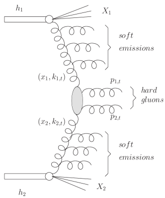
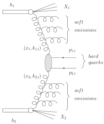
Figure 1: Typical diagrams for $k_{t}$-factorization approach to dijet production.

The $k_{t}$-factorization was originally proposed for heavy quark production original_kt_factorization . In recent years it was used to describe several high-energy processes, such as total cross section in virtual photon - proton scattering UGDF_HERA , heavy quark inclusive productionBS00 ; LSZ02 , heavy quark – heavy antiquark correlations LS04 ; LS06 , inclusive photon production LZ05_photon ; PS07 , inclusive pion production szczurek03 ; CS05 , Higgs boson Higgs or gauge boson KS04 production and dijet correlations in photoproduction SNSS01 and hadroproduction LO00 .

It is often claimed that the $k_{t}$-factorization approach includes implicitly some higher-order contributions of the standard collinear approach. This loose statement requires a better understanding and quantification.

Here we wish to address the problem of the relation between both approaches. We shall identify the regions of the phase space where the hard $2\to 3$ processes, not explicitly included in the leading-order $k_{t}$-factorization approach, dominate over the $2\to 2$ contributions calculated with UGDFs. We shall show how this depends on UGDFs used.

We shall concentrate on the region of relatively semi-hard jets, i.e. on the region related to the recently measured hadron-hadron correlations at RHIC. Here the resummation effects may be expected to be important. The resummation physics is addressed in our case through the $k_{t}$-factorization approach.

II Formalism

II.1 $2\to 2$ contributions with unintegrated parton distributions

It is known that at high energies, at midrapidities and not too large transverse momenta the jet production is dominated by (sub)processes initiated by gluons. In this paper we concentrate only on such processes. The region of forward/backward rapidities and/or processes with large rapidity gap between jets will be studied elsewhere. The cross section for the production of a pair of gluons or a pair of quark-antiquark can be written as

$$\frac{d\sigma(h_{1}h_{2}\rightarrow jj)}{d^{2}p_{1,t}d^{2}p_{2,t}} = \int dy_{1}dy_{2}\frac{d^{2}k_{1,t}}{\pi}\frac{d^{2}k_{2,t}}{\pi}\frac{1}{16\pi^{2}(x_{1}x_{2}s)^{2}}\overline{|{\cal M}(gg\rightarrow jj)|^{2}}$$ (1)

$$\cdot \delta^{2}(\overrightarrow{k}_{1,t}+\overrightarrow{k}_{2,t}-\overrightarrow{p}_{1,t}-\overrightarrow{p}_{2,t}){\cal F}(x_{1},k_{1,t}^{2}){\cal F}(x_{2},k_{2,t}^{2})\;,$$

where

$$x_{1}=\frac{m_{1,t}}{\sqrt{s}}\mathrm{e}^{+y_{1}}+\frac{m_{2,t}}{\sqrt{s}}\mathrm{e}^{+y_{2}}\;,$$ (2)

$$x_{2}=\frac{m_{1,t}}{\sqrt{s}}\mathrm{e}^{-y_{1}}+\frac{m_{2,t}}{\sqrt{s}}\mathrm{e}^{-y_{2}}\;.$$ (3)

The final partonic state is $jj=gg,q\bar{q}$. If one makes the following replacement

$${\cal F}_{1}(x_{1},k_{1,t}^{2})\rightarrow x_{1}g_{1}(x_{1})\delta(k_{1,t}^{2})$$ (4)

and

$${\cal F}_{2}(x_{2},k_{2,t}^{2})\rightarrow x_{2}g_{2}(x_{2})\delta(k_{2,t}^{2})$$ (5)

then one recovers the familiar standard collinear-factorization formula.

The inclusive invariant cross section for $g$ production can be written

$$\frac{d\sigma(h_{1}h_{2}\to j)}{dy_{1}d^{2}p_{1,t}}=2\int dy_{2}\frac{d^{2}k_{1,t}}{\pi}\frac{d^{2}k_{2,t}}{\pi}\left(...\right)|_{\vec{p}_{2,t}=\vec{k}_{1,t}+\vec{k}_{2,t}-\vec{p}_{1,t}}$$ (6)

and equivalently as

$$\frac{d\sigma(h_{1}h_{2}\to j)}{dy_{2}d^{2}p_{2,t}}=2\int dy_{1}\frac{d^{2}k_{1,t}}{\pi}\frac{d^{2}k_{2,t}}{\pi}\left(...\right)|_{\vec{p}_{1,t}=\vec{k}_{1,t}+\vec{k}_{2,t}-\vec{p}_{2,t}}\;.$$ (7)

Let us return to the coincidence cross section. The integration with the Dirac delta function in (1)

$$\int dy_{1}dy_{2}\frac{d^{2}k_{1,t}}{\pi}\frac{d^{2}k_{2,t}}{\pi}\left(...\right)\delta^{2}(...)\;.$$ (8)

can be performed by introducing the following new auxiliary variables:

$$\overrightarrow{Q}_{t} = \overrightarrow{k}_{1,t}+\overrightarrow{k}_{2,t}\;,$$

$$\overrightarrow{q}_{t} = \overrightarrow{k}_{1,t}-\overrightarrow{k}_{2,t}\;.$$ (9)

The jacobian of this transformation is:

$$\frac{\partial(\overrightarrow{Q}_{t},\overrightarrow{q}_{t})}{\partial(\overrightarrow{k}_{1,t},\overrightarrow{k}_{2,t})}=\begin{pmatrix}1&1\\ 1&-1\\ \end{pmatrix}\cdot\begin{pmatrix}1&1\\ 1&-1\\ \end{pmatrix}=2\cdot 2=4\;.$$ (10)

Then our initial cross section can be written as:

$$\frac{d\sigma(h_{1}h_{2}\rightarrow Q\bar{Q})}{d^{2}p_{1,t}d^{2}p_{2,t}}=\frac{1}{4}\int dy_{1}dy_{2}\;d^{2}Q_{t}d^{2}q_{t}\;(...)\;\delta^{2}(\overrightarrow{Q}_{t}-\overrightarrow{p}_{1,t}-\overrightarrow{p}_{2,t})$$ (11)

$$=\frac{1}{4}\int dy_{1}dy_{2}\;\underbrace{d^{2}q_{t}}\;\left(...\right)\;|_{\overrightarrow{Q}_{t}=\overrightarrow{P}_{t}}=$$ (12)

$$=\frac{1}{4}\int dy_{1}dy_{2}\;\overbrace{\underbrace{q_{t}dq_{t}}\;d\phi_{q_{t}}}\;\left(...\right)\;|_{\overrightarrow{Q}_{t}=\overrightarrow{P}_{t}}=$$ (13)

$$=\frac{1}{4}\int dy_{1}dy_{2}\;\overbrace{\frac{1}{2}dq_{t}^{2}\;d\phi_{q_{t}}}\;\left(...\right)\;|_{\overrightarrow{Q}_{t}=\overrightarrow{P}_{t}}\;.$$ (14)

Above $\vec{P}_{t}=\vec{p}_{1,t}+\vec{p}_{2,t}$. Different representations of the cross section are possible. If one is interested in the distribution of the sum of transverse momenta of the outgoing quarks, then it is convenient to write

$$d^{2}p_{1,t}\;d^{2}p_{2,t} = \frac{1}{4}d^{2}P_{t}d^{2}p_{t}=\frac{1}{4}d\phi_{P_{t}}P_{t}dP_{t}\;d\phi_{p_{t}}p_{t}dp_{t}$$ (15)

$$= \frac{1}{4}\;2\pi P_{t}dP_{t}\;d\phi_{p_{t}}p_{t}dp_{t}\;.$$

If one is interested in studying a two-dimensional map $p_{1,t}\times p_{2,t}$ then

$$d^{2}p_{1,t}\;d^{2}p_{2,t}=d\phi_{1}\;p_{1,t}dp_{1,t}\;d\phi_{2}\;p_{2,t}dp_{2,t}\;.$$ (16)

Then the two-dimensional map in jets transverse momenta can be written as

$$\frac{d\sigma(p_{1,t},p_{2,t})}{dp_{1,t}dp_{2,t}}=\int d\phi_{1}d\phi_{2}\;p_{1,t}p_{2,t}\;\int dy_{1}dy_{2}\;\frac{1}{4}q_{t}dq_{t}d\phi_{q_{t}}\left(...\right)\;.$$ (17)

The integral over $\phi_{1}$ and $\phi_{2}$ must be the most external one. The integral above is formally a 6-dimensional one. It is convenient to make the following transformation of variables

$$(\phi_{1},\phi_{2})\to\left(\phi_{+}=\phi_{1}+\phi_{2},\;\phi_{-}=\phi_{1}-\phi_{2}\right)\;,$$ (18)

where $\phi_{+}\in(0,4\pi)$ and $\phi_{-}\in(-2\pi,2\pi)$. Now the new domain $(\phi_{+},\phi_{-})$ is twice bigger than the original one $(\phi_{1},\phi_{2})$. The differential element

$$d\phi_{1}d\phi_{2}=\left(\frac{\partial\phi_{1}\partial\phi_{2}}{\partial\phi_{+}\partial\phi_{-}}\right)d\phi_{+}d\phi_{-}\;.$$ (19)

The transformation jacobian is:

$$\left(\frac{\partial\phi_{1}\partial\phi_{2}}{\partial\phi_{+}\partial\phi_{-}}\right)=\frac{1}{2}\;.$$ (20)

Then

$$d^{2}p_{1,t}\;d^{2}p_{2,t} = =p_{1,t}dp_{1,t}\;p_{2,t}dp_{2,t}{\frac{d\phi_{+}d\phi_{-}}{2}}$$ (21)

$$= p_{1,t}dp_{1,t}\;p_{2,t}dp_{2,t}\;2\pi d\phi_{-}\;.$$

The integrals in Eq.(17) can be written equivalently as

$$\frac{d\sigma(p_{1,t},p_{2,t})}{dp_{1,t}dp_{2,t}}=\frac{1}{2}\cdot\frac{1}{2}\int d\phi_{+}d\phi_{-}\;p_{1,t}p_{2,t}\;\int dy_{1}dy_{2}\;\frac{1}{4}q_{t}dq_{t}d\phi_{q_{t}}\left(...\right)\;.$$ (22)

The first factor of $\frac{1}{2}$ comes from the jacobian of the transformation and the second $\frac{1}{2}$ is due to the extra extension of the domain.

By symmetry, there is no dependence on $\phi_{+}$ and therefore the final result can be written as:

$$\frac{d\sigma(p_{1,t},p_{2,t})}{dp_{1,t}dp_{2,t}}=\frac{1}{2}\cdot\frac{1}{2}\cdot 4\pi\int d\phi_{-}\;p_{1,t}p_{2,t}\;\int dy_{1}dy_{2}\;\frac{1}{4}q_{t}dq_{t}d\phi_{q_{t}}\left(...\right)\;.$$ (23)

This 5-dimensional integral is now calculated for each point on the map $p_{1,t}\times p_{2,t}$. This formula can be also used to calculate a single particle spectrum of parton 1 and parton 2.

The matrix elements for 2 $\to$ 2 processes are discussed shortly in Appendix A. The analytical continuation of the standard on-shell matrix elements (see Appendix A) will be called in the following “on-shell approximation” for brevity. In Refs.LO00 ; O00 exact matrix elements for off-shell initial gluons were presented (see Appendix A). We have checked that the results obtained with the on-shell approximation and those obtained with the off-shell matrix elements are numerically almost identical. The deviations occur only for very virtual (large $k_{t}$) gluons where the contribution to the cross section is small for majority of UGDFs.

In the present calculation we shall include also components with gluon-quark and quark-gluon processes shown in Fig.2. In the next section we shall discuss how large are their contributions to the cross section.

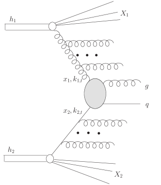
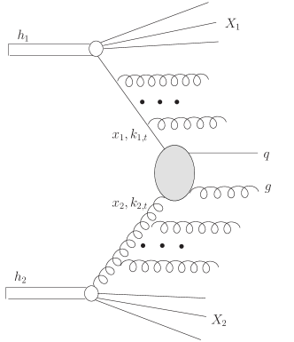
Figure 2: New $k_{t}$-factorization contributions included in the present paper

II.2 $2\to 3$ contributions in collinear-factorization approach

Up to now we have considered only processes with two explicit hard partons. In this section we shall discuss processes with three explicit hard partons. In Fig.3 we show a typical $2\to 3$ process. We also show kinematical variables needed in the description of the process. We select the particle 1 and 2 as those which correlations are studied. This is only formal as all possible combinations are considered in real calculations.

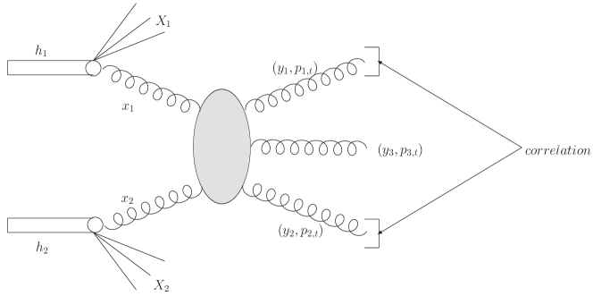
Figure 3: A typical diagram for $2\to 3$ contributions. The kinematical variables used are shown explicitly.

The cross section for $h_{1}h_{2}\to gggX$ can be calculated according to the standard parton model formula:

$$d\sigma(h_{1}h_{2}\to ggg)=\int dx_{1}dx_{2}\;g_{1}(x_{1},\mu^{2})g_{2}(x_{2},\mu^{2})\;d{\hat{\sigma}}(gg\to ggg)$$ (24)

The elementary cross section can be written as

$$d{\hat{\sigma}}(gg\to ggg)=\frac{1}{2{\hat{s}}}\overline{|{\cal M}_{gg\to ggg}|^{2}}dR_{3}\;.$$ (25)

The three-body phase space element is:

$$dR_{3}=\frac{d^{3}p_{1}}{2E_{1}(2\pi)^{3}}\frac{d^{3}p_{2}}{2E_{2}(2\pi)^{3}}\frac{d^{3}p_{3}}{2E_{3}(2\pi)^{3}}(2\pi)^{4}\delta^{4}(p_{a}+p_{b}-p_{1}-p_{2}-p_{3})\;,$$ (26)

It can be written in an equivalent way in terms of parton rapidities

$$dR_{3}=\frac{dy_{1}d^{2}p_{1,t}}{(4\pi)(2\pi)^{2}}\frac{dy_{2}d^{2}p_{2,t}}{(4\pi)(2\pi)^{2}}\frac{dy_{3}d^{2}p_{3,t}}{(4\pi)(2\pi)^{2}}(2\pi)^{4}\delta^{4}(p_{a}+p_{b}-p_{1}-p_{2}-p_{3})\;.$$ (27)

The last formula is useful for practical purposes. Now the cross section for hadronic collisions can be written in terms of $2\to 3$ matrix element as

$$d\sigma=dy_{1}d^{2}p_{1,t}dy_{2}d^{2}p_{2,t}dy_{3}\cdot\frac{1}{(4\pi)^{3}(2\pi)^{2}}\;\frac{1}{\hat{s}^{2}}\;x_{1}f_{1}(x_{1},\mu_{f}^{2})x_{2}f_{2}(x_{2},\mu_{f}^{2})\;\overline{|{\cal M}_{2\to 3}|^{2}}\;,$$ (28)

where the longitudinal momentum fractions are evaluated as

$$x_{1} = \frac{p_{1,t}}{\sqrt{s}}\exp(+y_{1})+\frac{p_{2,t}}{\sqrt{s}}\exp(+y_{2})+\frac{p_{3,t}}{\sqrt{s}}\exp(+y_{3})\;,$$

$$x_{2} = \frac{p_{1,t}}{\sqrt{s}}\exp(-y_{1})+\frac{p_{2,t}}{\sqrt{s}}\exp(-y_{2})+\frac{p_{3,t}}{\sqrt{s}}\exp(-y_{3})\;.$$ (29)

Repeating similar steps as for $2\to 2$ processes we get finally:

$$d\sigma=\frac{1}{64\pi^{4}\hat{s}^{2}}\;x_{1}f_{1}(x_{1},\mu_{f}^{2})x_{2}f_{2}(x_{2},\mu_{f}^{2})\;\overline{|{\cal M}_{2\to 3}|^{2}}p_{1,t}dp_{1,t}p_{2,t}dp_{2,t}d\phi_{-}dy_{1}dy_{2}dy_{3}\;,$$ (30)

where $\phi_{-}$ is restricted to the interval $(0,\pi)$. The last formula is very useful in calculating the cross section for particle 1 and particle 2 correlations.

II.3 Unintegrated gluon distributions

In general, there are no simple relations between unintegrated and integrated parton distributions. Some of UPDFs in the literature are obtained based on familiar collinear distributions, some are obtained by solving evolution equations, some are just modelled or some are even parametrized. A brief review of unintegrated gluon distributions (UGDFs) that will be used here can be found in Ref.LS06 . We shall not repeat all details concerning those UGDFs here. We shall discuss in more details only approaches which treat unintegrated quark/antiquark distributions.

In some of approaches one imposes the following relation between the standard collinear distributions and UPDFs:

$$a(x,\mu^{2})=\int_{0}^{\mu^{2}}f_{a}(x,{\mathrm{\bf k}}_{t}^{2},\mu^{2})\frac{d{\mathrm{\bf k}}_{t}^{2}}{{\mathrm{\bf k}}_{t}^{2}}\;,$$ (31)

where $a=xq$ or $a=xg$.

Since familiar collinear distributions satisfy sum rules, one can define and test analogous sum rules for UPDFs. We shall discuss this issue in more detail in a separate section.

Due to its simplicity the Gaussian smearing of initial transverse momenta is a good reference for other approaches. It allows to study phenomenologically the role of transverse momenta in several high-energy processes. We define a simple unintegrated parton distributions:

$${\cal F}_{i}^{Gauss}(x,k^{2},\mu_{F}^{2})=xp_{i}^{coll}(x,\mu_{F}^{2})\cdot f_{Gauss}(k^{2})\;,$$ (32)

where $p_{i}^{coll}(x,\mu_{F}^{2})$ are standard collinear (integrated) parton distribution ($i=g,q,\bar{q}$) and $f_{Gauss}(k^{2})$ is a Gaussian two-dimensional function:

$$f_{Gauss}(k^{2})=\frac{1}{2\pi\sigma_{0}^{2}}\exp\left(-k_{t}^{2}/2\sigma_{0}^{2}\right)\frac{1}{\pi}\;.$$ (33)

The UPDFs defined by Eq.(32) and (33) is normalized such that:

$$\int{\cal F}_{i}^{Gauss}(x,k^{2},\mu_{F}^{2})\;dk^{2}=xp_{i}^{coll}(x,\mu_{F}^{2})\;.$$ (34)

Kwieciński has shown that the evolution equations for unintegrated parton distributions takes a particularly simple form in the variable conjugated to the parton transverse momentum. In the impact-parameter space the Kwieciński equations takes the following relatively simple form

$$\begin{split}{\partial{\tilde{\cal F}_{NS}(x,b,\mu^{2})}\over\partial\mu^{2}}&={\alpha_{s}(\mu^{2})\over 2\pi\mu^{2}}\int_{0}^{1}dz\,P_{qq}(z)\bigg{[}\Theta(z-x)\,J_{0}((1-z)\mu b)\,{\tilde{\cal F}_{NS}\left({x\over z},b,\mu^{2}\right)}\\ &-{\tilde{\cal F}_{NS}(x,b,\mu^{2})}\bigg{]}\;,\\ {\partial{\tilde{\cal F}_{S}(x,b,\mu^{2})}\over\partial\mu^{2}}&={\alpha_{s}(\mu^{2})\over 2\pi\mu^{2}}\int_{0}^{1}dz\bigg{\{}\Theta(z-x)\,J_{0}((1-z)\mu b)\bigg{[}P_{qq}(z)\,{\tilde{\cal F}_{S}\left({x\over z},b,\mu^{2}\right)}\\ &+P_{qg}(z)\,{\tilde{\cal F}_{G}\left({x\over z},b,\mu^{2}\right)}\bigg{]}-[zP_{qq}(z)+zP_{gq}(z)]\,{\tilde{\cal F}_{S}(x,b,\mu^{2})}\bigg{\}}\;,\\ {\partial{\tilde{\cal F}_{G}(x,b,\mu^{2})}\over\partial\mu^{2}}&={\alpha_{s}(\mu^{2})\over 2\pi\mu^{2}}\int_{0}^{1}dz\bigg{\{}\Theta(z-x)\,J_{0}((1-z)\mu b)\bigg{[}P_{gq}(z)\,{\tilde{\cal F}_{S}\left({x\over z},b,\mu^{2}\right)}\\ &+P_{gg}(z)\,{\tilde{\cal F}_{G}\left({x\over z},b,\mu^{2}\right)}\bigg{]}-[zP_{gg}(z)+zP_{qg}(z)]\,{\tilde{\cal F}_{G}(x,b,\mu^{2})}\bigg{\}}\;.\end{split}$$ (35)

We have introduced here the short-hand notation

$$\begin{split}\tilde{\cal F}_{NS}&=\tilde{\cal F}_{u}-\tilde{\cal F}_{\bar{u}},\;\;\tilde{\cal F}_{d}-\tilde{\cal F}_{\bar{d}}\;,\\ \tilde{\cal F}_{S}&=\tilde{\cal F}_{u}+\tilde{\cal F}_{\bar{u}}+\tilde{\cal F}_{d}+\tilde{\cal F}_{\bar{d}}+\tilde{\cal F}_{s}+\tilde{\cal F}_{\bar{s}}\;.\end{split}$$ (36)

The unintegrated parton distributions in the impact factor representation are related to the familiar collinear distributions as follows

$$\tilde{\cal F}_{k}(x,b=0,\mu^{2})=\frac{x}{2}p_{k}(x,\mu^{2})\;.$$ (37)

On the other hand, the transverse momentum dependent UPDFs are related to the integrated parton distributions as

$$xp_{k}(x,\mu^{2})=\int_{0}^{\infty}dk_{t}^{2}\;{\cal F}_{k}(x,k_{t}^{2},\mu^{2})\;.$$ (38)

The two possible representations are interrelated via Fourier-Bessel transform

$$\begin{split}&{{\cal F}_{k}(x,k_{t}^{2},\mu^{2})}=\int_{0}^{\infty}db\;bJ_{0}(k_{t}b){{\tilde{\cal F}}_{k}(x,b,\mu^{2})}\;,\\ &{{\tilde{\cal F}}_{k}(x,b,\mu^{2})}=\int_{0}^{\infty}dk_{t}\;k_{t}J_{0}(k_{t}b){{\cal F}_{k}(x,k_{t}^{2},\mu^{2})}\;.\end{split}$$ (39)

The index k above numerates either gluons (k=0), quarks (k$>$ 0) or antiquarks (k$<$ 0).

While physically ${\cal F}_{k}(x,k_{t}^{2},\mu^{2})$ should be positive, there is no obvious reason for such a limitation for $\tilde{\cal F}_{k}(x,b,\mu^{2})$.

In the following we use leading-order parton distributions from Ref.GRV98 as the initial condition for QCD evolution. The set of integro-differential equations in b-space was solved by the method based on the discretisation made with the help of the Chebyshev polynomials (see kwiecinski ). Then the unintegrated parton distributions were put on a grid in $x$, $b$ and $\mu^{2}$ and the grid was used in practical applications for Chebyshev interpolation.

For the calculation of jet correlations here the parton distributions in momentum space are more useful. These calculation requires a time-consuming multi-dimensional integration. An explicit calculation of the Kwieciński UPDFs via Fourier transform for needed in the main calculation values of $(x_{1},k_{1,t}^{2})$ and $(x_{2},k_{2,t}^{2})$ (see next section) is not possible. Therefore auxiliary grids of the momentum-representation UPDFs are prepared before the actual calculation of the cross sections. These grids are then used via a two-dimensional interpolation in the spaces $(x_{1},k_{1,t}^{2})$ and $(x_{2},k_{2,t}^{2})$ associated with each of the two incoming partons.

III Results

Let us concentrate first on $2\to 2$ processes calculated with the inclusion of initial transverse momenta. We shall include the following four (sub)processes:

• gluon+gluon $\to$ gluon+gluon (called diagram $A_{1}$, see Fig.1a)

• gluon+gluon $\to$ quark+antiquark (called diagram $A_{2}$, see Fig.1b)

• gluon+(anti)quark $\to$ gluon+(anti)quark (called diagram $B_{1}$, see Fig.2a)

• (anti)quark+gluon $\to$ (anti)quark+gluon (called diagram $B_{2}$, see Fig.2b)

Only first two were included recently in the $k_{t}$-factorization approach LO00 ; Bartels . The papers in the literature have been concentrated on large energies, i.e. on such cases when only gluons come into game. We shall show that at present subasymptotic energies (RHIC, Tevatron) also the last two must be included, even at midrapidities. Similar conclusion was drawn recently for inclusive pion distributions at RHIC CS05 .

Figure 4: Two-dimensional distributions in $p_{1,t}$ and $p_{2,t}$ for different subprocesses $gg\to gg$ (left upper) $gg\to q\bar{q}$ (right upper), $gq\to gq$ (left lower) and $qg\to qg$ (right lower). In this calculation W = 200 GeV and Kwieciński UPDFs with exponential nonperturbative form factor ($b_{0}$ = 1 GeV^-1) and $\mu^{2}$ = 100 GeV² were used. Here integration over full range of parton rapidities was made.

In Fig.4 we show two-dimensional maps in $(p_{1,t},p_{2,t})$ for listed above subprocesses. Only very few approaches in the literature include both gluons and quarks and antiquarks. In the calculation above we have used Kwieciński UPDFs with exponential nonperturbative form factor ($b_{0}$ = 1 GeV^-1) and the factorization scale $\mu^{2}=(p_{t,min}+p_{t,max})^{2}/4$ = 100 GeV².

Figure 5: Two-dimensional distributions of fractional contributions of different subprocesses as a function of $y_{1}$ and $y_{2}$ for $gg\to gg$ (left upper) $gg\to q\bar{q}$ (right upper), $gq\to gq$ (left lower) and $qg\to qg$ (right lower). In this calculation W = 200 GeV and Kwieciński UPDFs with exponential nonperturbative form factor and $b_{0}$ = 1 GeV^-1 were used. The integration is made for jets from the transverse momentum interval: 5 GeV $<p_{1,t},p_{2,t}<$ 20 GeV.

In Fig.5 we show a fractional contributions (individual component to the sum of all four components) of the above four processes on the two-dimensional map $(y_{1},y_{2})$. One point here requires a better clarification. Experimentally it is not possible to distinguish gluon and quark/antiquark jets. Therefore in our calculation of the $(y_{1},y_{2})$ dependence one has to symmetrize the cross section (not the amplitude) with respect to gluon – quark/antiquark exchange ($y_{1}\to y_{2},y_{2}\to y_{1}$). This can be done technically by exchanging $\hat{t}$ and $\hat{u}$ variables in the matrix element squared. While at midrapidities the contribution of diagram $B_{1}$ + $B_{2}$ is comparable to the diagram $A_{1}$, at larger rapidities the contributions of diagrams of the type B dominate. The contribution of diagram $A_{2}$ is relatively small in the whole phase space. When calculating the contributions of the diagram $A_{1}$ and $A_{2}$ one has to be careful about collinear singularity which leads to a significant enhancement of the cross section at $\phi_{-}$=0 and $y_{1}=y_{2}$, i.e. in the one jet case. This is particularly important for the matrix elements obtained by the naive analytic continuation from the formula for on-shell initial partons. The effect can be, however, easily eliminated with the jet-cone separation algorithm discussed in Appendix D.

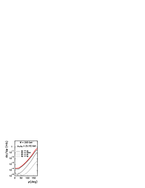
Figure 6: The angular correlations for all four components: $gg\to gg$ (solid), $gg\to q\bar{q}$ (dashed) and $gq\to gq$ = $qg\to qg$ (dash-dotted). The calculation is performed with the Kwieciński UPDFs and $b_{0}$ = 1 GeV^-1. The integration is made for jets from the transverse momentum interval: 5 GeV $<p_{1,t},p_{2,t}<$ 15 GeV and from the rapidity interval: -4 $<y_{1},y_{2}<$ 4.

For completeness in Fig.6 we show azimuthal angle dependence of the cross section for all four components. There is no sizeable difference in the shape of azimuthal distribution for different components.

The Kwieciński approach allows to separate the unknown perturbative effects incorporated via nonperturbative form factors and the genuine effects of QCD evolution. The Kwieciński distributions have two external parameters:

• the parameter $b_{0}$ responsible for nonperturbative effects, such as primordial distribution of partons in the nucleon,

• the evolution scale $\mu_{F}^{2}$ responsible for the soft resummation effects.

While the latter can be identified physically with characteristic kinematical quantities in the process $\mu_{F}^{2}\sim p_{1,t}^{2},p_{2,t}^{2}$, the first one is of nonperturbative origin and cannot be calculated from first principles. The shapes of distributions depends, however, strongly on the value of the parameter $b_{0}$. This is demonstrated in Fig.7 for the $gg\to gg$ subprocess. The smaller $b_{0}$ the bigger decorrelation in azimuthal angle can be observed. In Fig.7 we show also the role of the evolution scale in the Kwieciński distributions. The QCD evolution embedded in the Kwieciński evolution equations populate larger transverse momenta of partons entering the hard process. This significantly increases the initial (nonperturbative) decorrelation in azimuth. For transverse momenta of the order of $\sim$ 10 GeV the effect of evolution is of the same order of magnitude as the effect due to nonperturbative physics. For larger scales of the order of $\mu_{F}^{2}\sim$ 100 GeV², more adequate for jet production, the initial condition is of minor importance and the effect of decorrelation is dominated by the evolution. Asymptotically (infinite scales) there is no dependence on the initial condition provided reasonable initial conditions are taken.

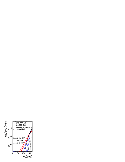
Figure 7: The azimuthal correlations for the $gg\to gg$ component obtained with the Kwieciński UGDFs for different values of the nonperturbative parameter $b_{0}$ and for different evolution scales $\mu^{2}$ = 10 (on line blue), 100 (on line red) GeV². The initial distributions (without evolution) are shown for reference by black lines.

In Fig.8 we show azimuthal-angle correlations for the dominant at midrapidity $gg\to gg$ component for different UGDFs from the literature. Rather different results are obtained for different UGDFs. In principle, experimental results could select the “best” UGDF. We do not need to mention that such measurements are not easy at RHIC and rather hadron correlations are studied instead of jet correlations.

Figure 8: The azimuthal correlations for the $gg\to gg$ component obtained for different UGDFs from the literature. The Kwieciński distribution is for $b_{0}$ = 1 GeV^-1 and $\mu^{2}$ = 100 GeV².

Figure 9: Two-jet correlations for a $2\to 3$ $gg\to ggg$ component for RHIC energy W = 200 GeV. The soft singularities are shown as ridges. The pQCD calculations are reliable outside of the regions of ridges.

Before we start presenting further more detailed results let us concentrate on NLO calculation . In Fig.9 we show the results of a naive calculation, on the $(p_{1,t},p_{2,t})$ plane where soft divergences are shown explicitly. One clearly sees 3 sharp ridges: along x and y axes as well as along the diagonal. While the ridges along x and y axis can be easily eliminated by imposing cuts on $p_{1,t}$ and $p_{2,t}$, i.e. on jets taken in the analysis of correlations. The elimination of the third ridge is more subtle and will be discussed somewhat later. Sometimes asymmetric cuts on jet transverse momenta are imposed in order to avoid technical problems.

Let us start from presenting the results on the plane $(p_{1,t},p_{2,t})$. In Fig.10 we show the maps for different choices of UGDFs and for $2\to 3$ processes in the broad range of transverse momenta 5 GeV $<p_{1,t},p_{2,t}<$ 20 GeV for the RHIC energy W = 200 GeV. In this calculation we have not imposed any particular cuts on rapidities. We have not imposed also any cut on the transverse momentum of the unobserved third jet in the case of $2\to 3$ calculation. The small transverse momenta of the third jet contribute to the sharp ridge along the diagonal $p_{1,t}=p_{2,t}$. Naturally this is therefore very difficult to distinguish these three-parton states from standard two jet events. In principle, the ridge can be eliminated by imposing a cut on the transverse momentum of the third (unobserved) parton. There are also other methods to eliminate the ridge and underlying soft processes which will be discussed somewhat later.

In Fig.8 we show corresponding distributions in azimuthal angle $\phi_{-}$. Very different azimuthal correlation functions are obtained for different UGDFs. The NLO azimuthal angle correlation function exceeds those obtained in the $k_{t}$-factorization approach for $\phi_{-}<$ 90^o.

When calculating dijet correlations in the standard NLO ($2\to 3$) approach we have taken all possible dijet combinations. This is different from what is usually taken in experiments D0_data , where correlation between leading jets are studied. In our notation this means $p_{3,t}<p_{1,t}$ and $p_{3,t}<p_{2,t}$. When imposing such extra condition on our NLO calculation we get the dash-dotted curve in Fig.8. In this case $d\sigma/d\phi_{-}=0$ for $\phi_{-}<\tfrac{2}{3}\pi$. This vanishing of the cross section is of purely kinematical origin. Since in the $k_{t}$-factorization calculation only two jets are explicit, there is no such an effect in this case. This means that the region of $\phi_{-}<\frac{2}{3}\pi$ should be useful to test models of UGDFs. For completeness in Fig.12 we show a two-dimensional plot $(p_{1,t},p_{2,t})$ with imposing the leading-jet condition. Surprisingly the leading-jet condition removes a big part of the two-dimensional space. In particular, regions with $p_{2,t}>2p_{1,t}$ (NLO-forbidden region1) and $p_{1,t}>2p_{2,t}$ (NLO-forbidden region2) cannot be populated via $2\to 3$ subprocess . There are no such limitations for $2\to 4$, $2\to 5$ and even higher-order processes. Therefore measurements in “NLO-forbidden” regions of the $(p_{1,t},p_{2,t})$ plane would test higher-order terms of the standard collinear pQCD. These are also regions where UGDFs can be tested, provided that not too big transverse momenta of jets taken into the correlation in order to assure the dominance of gluon-initiated processes (for larger transverse momenta and/or forward/backward rapidities one has to include also quark/antiquark initiated processes via unintegrated quark/antiquark distributions).

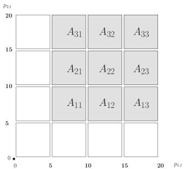
Figure 13: Definition of windows in $(p_{1,t},p_{2,t})$ plane for a further use.

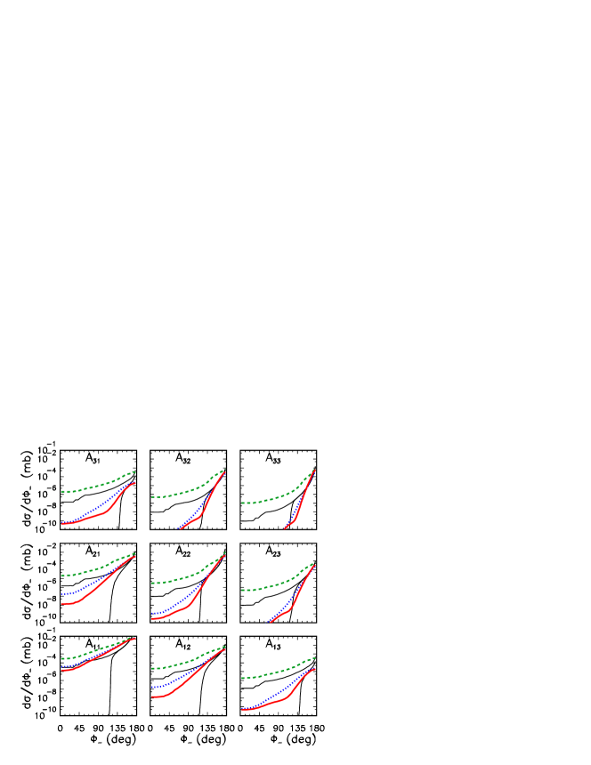
Figure 14: Dijet azimuthal correlations $d\sigma/d\phi_{-}$ for different windows in the $(p_{1,t},p_{2,t})$ plane as a function of relative azimuthal angle $\phi_{-}$ between outgoing jets for RHIC energy W = 200 GeV. The jet-cone radius $R_{12}$ = 1 was used here in addition to separate jets. The notation here is the same as in Fig.8.

Can we gain a new information correlating the space of azimuthal angle $(\phi_{-})$ and the space spanned by the lengths of transverse momenta $(p_{1,t},p_{2,t})$ ? In particular, it is interesting how the jet azimuthal correlations depend on a region of $(p_{1,t},p_{2,t})$. For this purpose in Fig.13 we define several regions in $(p_{1,t},p_{2,t})$, called windows, for easy reference in the following. They have been named $A_{ij}$ for future easy notation. In Fig.14 we show angular azimuthal correlations for each of these regions separately. While at small transverse momenta the cross section obtained with $2\to 2$ $k_{t}$-factorization and $2\to 3$ collinear-factorization approaches are of similar order, at larger transverse momenta and far from the diagonal $p_{1,t}=p_{2,t}$ the cross section is dominated by the genuine next-to-leading order processes. In these regions the standard higher-order collinear-factorization approach seems to be the best, and probably the only, method to study dijet azimuthal-angle correlations.

Cuts on $p_{1,t}$ and $p_{2,t}$ remove a big part of soft singularities, leaving only region of $p_{1,t}\approx p_{2,t}$. In order to eliminate the regions where the pQCD calculation does not apply we suggest to exclude the region shown in diagram 15 which is equivalent to including the following cuts on the lengths of transverse momenta of the jets taken into account in the correlations:

$$|p_{1,t}-p_{2,t}|>\Delta_{s}$$ (40)

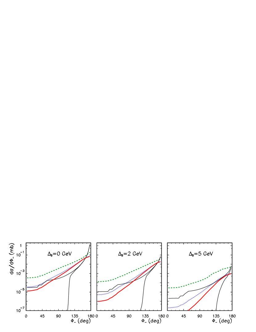
Figure 16: Azimuthal angular correlations for different values of the parameter $\Delta_{s}$ = 0, 2, 5 GeV. Different UGDF are used. The notation here is the same as previously. The jet-cone radius $R_{12}$ = 1 was used in addition to separate jets. The notation here is the same as in Fig.8.

In Fig.16 we show the distribution of the cross section in azimuthal angle for different (scalar) cuts $\Delta_{s}$ = 0,2,5 GeV. We have also tried another way to remove singularities:

$$|\vec{p}_{1,t}+\vec{p}_{2,t}|>\Delta_{v}$$ (41)

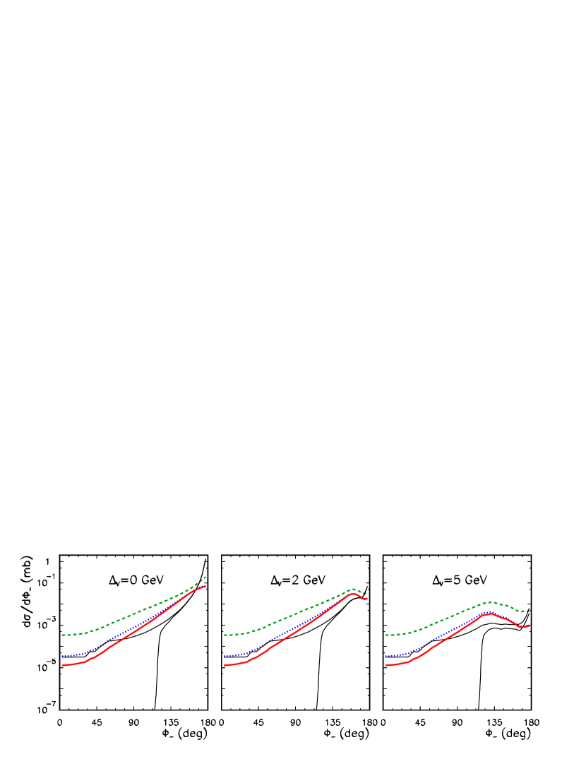
Figure 17: Azimuthal angular correlations for different values of the parameter $\Delta_{v}$ = 0, 2, 5 GeV. Different UGDF are used. The notation here is the same as previously. The jet-cone radius $R_{12}$ = 1 was used in addition to separate jets. The notation here is the same as in Fig.8.

In Fig.17 we show the distribution of the cross section in azimuthal angle for different (vector) cuts $\Delta_{v}$ = 0,2,5 GeV. These results are very similar to those obtained with scalar cuts.

Both scalar and vector cuts remove efficiently the singularity of the collinear 2$\to$3 contribution at $\phi_{-}=\pi$. If too big values of $\Delta_{s}$ or $\Delta_{v}$ are used the cross section of the $k_{t}$-factorization 2$\to$2 contribution is reduced considerably.

IV Discussion and Conclusions

Motivated by the recent experimental results of hadron-hadron correlations at RHIC we have discussed dijet correlations in proton-proton collisions. We have considered and compared results obtained with collinear next-to-leading order approach and leading-order $k_{t}$-factorization approach.

In comparison to recent works in the framework of $k_{t}$-factorization approach, we have included two new mechanisms based on $gq\to gq$ and $qg\to qg$ hard subprocesses. This was done based on the Kwieciński unintegrated parton distributions. We find that the new terms give significant contribution at RHIC energies. In general, the results of the $k_{t}$-factorization approach depend on UGDFs/UPDFs used, i.e. on approximation and assumptions made in their derivation.

An interesting observation has been made for azimuthal angle correlations. At relatively small transverse momenta ($p_{t}\sim$ 5–10 GeV) the $2\to 2$ subprocesses, not contributing to the correlation function in the collinear approach, dominate over $2\to 3$ components. The latter dominate only at larger transverse momenta, i.e. in the traditional jet region.

The results obtained in the standard NLO approach depend significantly whether we consider correlations of any jets or correlations of only leading jets. In the NLO approach one obtains $\frac{d\sigma}{d\phi_{-}}$ = 0 if $\phi_{-}<\tfrac{2}{3}\pi$ for leading jets as a result of a kinematical constraint. Similarly $\frac{d\sigma}{dp_{1,t}dp_{2,t}}$ = 0 if $p_{1,t}>2p_{2,t}$ or $p_{2,t}>2p_{1,t}$.

There is no such a constraint in the $k_{t}$-factorization approach which gives a nonvanishing cross section at small relative azimuthal angles between leading jets and transverse-momentum asymmetric configurations. We conclude that in these regions the $k_{t}$-factorization approach is a good and efficient tool for the description of leading-jet correlations. Rather different results are obtained with different UGDFs which opens a possibility to verify them experimentally. Alternatively, the NLO-forbidden configurations can be described only by higher-order (NNLO and higher-order) terms. We do not need to mention that this is a rather difficult and technically involved computation.

On the contrary, in the case of correlations of any unrestricted jets (all possible dijet combinations) the NLO cross section exceeds the cross section obtained in the $k_{t}$-factorization approach with different UGDFs. This is therefore a domain of the standard fixed-order pQCD. We recommend such an analysis as an alternative to study leading-jet correlations. In principle, such an analysis could be done for the already collected Tevatron data.

What are consequences for particle-particle correlations measured recently at RHIC requires a separate dedicated analysis. Here the so-called leading particles may come both from leading and non-leading jets. This requires taking into account the jet fragmentation process. We leave this analysis for a separate study.

V Appendices

V.1 Matrix elements for $2\to 2$ processes with initial off-shell gluons

In this paper we shall include the following $2\to 2$ processes with at least one gluon in the initial state:
(a) $gg\to gg$, (b) $gg\to q\bar{q}$, (c) $gq\to gq$, (d) $qg\to qg$, i.e. processes giving significant contributions for inclusive jet production at relatively small jet transverse momenta and midrapidities SB98 . The last two processes were not included in Refs.LO00 , Bartels . We shall show that at RHIC energies they give contributions similar (or even larger) to the contribution of the asymptotically dominant $gg\to gg$ subprocess.

The matrix elements for on-shell initial gluons/partons read (see e.g.BP_book )

$$\overline{|{\cal M}_{gg\to gg}|^{2}} = \frac{9}{2}g_{s}^{4}\left(3-\frac{\hat{t}\hat{u}}{\hat{s}^{2}}-\frac{\hat{s}\hat{u}}{\hat{t}^{2}}-\frac{\hat{s}\hat{t}}{\hat{u}^{2}}\right)\;,$$

$$\overline{|{\cal M}_{gg\to q\bar{q}}|^{2}} = \frac{1}{8}g_{s}^{4}\left(6\frac{\hat{t}\hat{u}}{\hat{s}^{2}}+\frac{4}{3}\frac{\hat{u}}{\hat{t}}+\frac{4}{3}\frac{\hat{t}}{\hat{u}}+3\frac{\hat{t}}{\hat{s}}+3\frac{\hat{u}}{\hat{s}}\right)\;,$$

$$\overline{|{\cal M}_{gq\to gq}|^{2}} = g_{s}^{4}\left(-\frac{4}{9}\frac{\hat{s}^{2}+\hat{u}^{2}}{\hat{s}\hat{u}}+\frac{\hat{u}^{2}+\hat{s}^{2}}{\hat{t}^{2}}\right)\;,$$

$$\overline{|{\cal M}_{qg\to qg}|^{2}} = g_{s}^{4}\left(-\frac{4}{9}\frac{\hat{s}^{2}+\hat{t}^{2}}{\hat{s}\hat{t}}+\frac{\hat{t}^{2}+\hat{s}^{2}}{\hat{u}^{2}}\right)\;.$$ (42)

For on-shell initial gluons (partons) $\hat{s}+\hat{t}+\hat{u}=0$.

The matrix elements for off-shell initial gluons are obtained by using the same formulas but with $\hat{s},\hat{t},\hat{u}$ calculated including off-shell initial kinematics. In this case $\hat{s}+\hat{t}+\hat{u}=k_{1}^{2}+k_{2}^{2}$, where $k_{1}^{2},k_{2}^{2}<$ 0 are virtualities of the initial gluons. Our prescription can be treated as a smooth analytic continuation of the on-shell formula off mass shell. With our choice of initial gluon four-momenta $k_{1}^{2}=-k_{1,t}^{2}$ and $k_{2}^{2}=-k_{2,t}^{2}$.

In Refs.LO00 ; O00 another formula which includes off-shellness of initial gluons was presented

$$\frac{d\sigma}{d^{2}p_{1,t}d^{2}p_{2,t}dy_{1}dy_{2}}=\int\frac{d^{2}k_{1,t}}{\pi}\frac{d^{2}k_{2,t}}{\pi}{\cal F}(x_{1},k_{1t}^{2})\frac{d\sigma}{d^{2}p_{1,t}d^{2}p_{2,t}}{\cal F}(x_{2},k_{2,t}^{2})\;,$$ (43)

where

$$\frac{d\sigma}{d^{2}p_{1,t}d^{2}p_{2,t}}=2\frac{N_{c}^{2}}{(N_{c}^{2}-1)}\;\alpha_{s}^{2}(\mu_{r})\;\frac{1}{k_{1,t}^{2}k_{2,t}^{2}}\;\delta^{2}(\vec{k}_{1,t}+\vec{k}_{2,t}-\vec{p}_{1,t}-\vec{p}_{2,t})\;{\cal A}\;.$$ (44)

The factor ${\cal A}$ is a function of momenta entering the hard process ${\cal A}={\cal A}(\hat{s},\hat{t},\hat{u},k_{1,t},k_{2,t})$ (see LO00 ). The factor A has been rederived recently in Ref. Bartels and the result of Leonidov and Ostrovsky was confirmed.

Please note a different convention of UGDF in our paper (${\cal F}$) with those in Refs.LO00 ; O00 ($f$). The UGDFs in the two conventions are related to each other as

$${\cal F}(x,k_{t}^{2})=f(x,k_{t}^{2})/k_{t}^{2}\;.$$ (45)

In order to eliminate the delta function in Eq.(44) we can use the same tricks as in the previous section.

The formula of Leonidov and Ostrovsky is equivalent to our formula if we define:

$$\overline{|{\cal M}|^{2}}_{off-shell}=16\pi^{2}(x_{1}x_{2}s)^{2}\frac{N_{c}^{2}-1}{2N_{c}^{2}}\alpha_{s}^{2}\frac{\cal A}{k_{1,t}^{2}k_{2,t}^{2}}\;.$$ (46)

V.2 Matrix elements for $2\to 3$ processes

In this subsection we list the squared matrix elements averaged and summed over initial and final spins and colors used to calculate the contribution of the $2\to 3$ partonic processes (For useful reference see e.g.berends ; BP_book ).

For the $gg\to ggg$ process ($k_{1}+k_{2}\to k_{3}+k_{4}+k_{5}$) the squared matrix element is

$$\begin{split}\overline{|{\cal M}|^{2}}&=\frac{1}{2}g_{s}^{6}\frac{N_{c}^{3}}{N_{c}^{2}-1}\\ \bigl{[}&(12345)+(12354)+(12435)+(12453)+(12534)+(12543)+\\ &(13245)+(13254)+(13425)+(13524)+(12453)+(14325)\bigr{]}\\ &\times\sum_{i<j}(k_{i}k_{j})/\prod_{i<j}(k_{i}k_{j})\;,\end{split}$$ (47)

where $(ijlmn)\equiv(k_{i}k_{j})(k_{j}k_{l})(k_{l}k_{m})(k_{m}k_{n})(k_{n}k_{i})$.

It is useful to calculate matrix element for the process $q\bar{q}\to ggg$. The squared matrix elements for other processes can be obtained by crossing the squared matrix element for the process $q\bar{q}\to ggg$ ($p_{a}+p_{b}\to k_{1}+k_{2}+k_{3}$)

$$\begin{split}\overline{|{\cal M}|^{2}}&=g_{s}^{6}\frac{N_{c}^{2}-1}{4N_{c}^{4}}\\ &\sum_{i}^{3}a_{i}b_{i}(a_{i}^{2}+b_{i}^{2})/(a_{1}a_{2}a_{3}b_{1}b_{2}b_{3})\\ \times&\Biggl{[}\frac{\hat{s}}{2}+N_{c}^{2}\left(\frac{\hat{s}}{2}-\frac{a_{1}b_{2}+a_{2}b_{1}}{(k_{1}k_{2})}-\frac{a_{2}b_{3}+a_{3}b_{2}}{(k_{2}k_{3})}-\frac{a_{3}b_{1}+a_{1}b_{3}}{(k_{3}k_{1})}\right)\\ &+\frac{2N^{4}}{\hat{s}}\left(\frac{a_{3}b_{3}(a_{1}b_{2}+a_{2}b_{1})}{(k_{2}k_{3})(k_{3}k_{1})}+\frac{a_{1}b_{1}(a_{2}b_{3}+a_{3}b_{2})}{(k_{3}k_{1})(k_{1}k_{2})}+\frac{a_{2}b_{2}(a_{3}b_{1}+a_{1}b_{3})}{(k_{1}k_{2})(k_{2}k_{3})}\right)\Biggr{]}\;,\end{split}$$ (48)

where the quantities $a_{i}$ and $b_{i}$ are defined as:

$$a_{i}\equiv(p_{a}k_{i})\;,$$

$$b_{i}\equiv(p_{b}k_{i})\;.$$ (49)

The matrix element for the process $gg\to q\bar{q}g$ is obtained from that of $q\bar{q}\to ggg$ by appropriate crossing:

$$\overline{|{\cal M}|^{2}}_{gg\to q\bar{q}g}(k_{1},k_{2},k_{3},k_{4},k_{5})=\frac{9}{64}\cdot\overline{|{\cal M}|^{2}}_{q\bar{q}\to ggg}(-k_{4},-k_{3},-k_{1},-k_{2},k_{5})\;.$$ (50)

We sum over 3 final flavours (f = u, d, s).

For the $qg\to qgg$ process

$$\overline{|{\cal M}|^{2}}_{qg\to qgg}(k_{1},k_{2},k_{3},k_{4},k_{5})=\left(-\frac{3}{8}\right)\cdot\overline{|{\cal M}|^{2}}_{q\bar{q}\to ggg}(k_{1},-k_{3},-k_{2},k_{4},k_{5})$$ (51)

and finally for the process $g\bar{q}\to\bar{q}gg$

$$\overline{|{\cal M}|^{2}}_{g\bar{q}\to\bar{q}gg}(k_{1},k_{2},k_{3},k_{4},k_{5})=\left(-\frac{3}{8}\right)\cdot\overline{|{\cal M}|^{2}}_{q\bar{q}\to ggg}(-k_{3},k_{2},-k_{1},k_{4},k_{5})\;.$$ (52)

The squared matrix elements are used then in formula (24). The contributions with two quark/antiquark initiated processes are important at extremely large rapidities. They will be neglected in the present analysis where we concentrate on midrapidities.

V.3 Running $\alpha_{s}$

The treatment of the running coupling constants in $2\to 2$ and $2\to 3$ subprocesses is important in numerical evaluation of the cross section.

For the $2\to 2$ case we shall try several prescriptions:
($\alpha_{1}$) $\alpha_{s}^{2}=\alpha_{s}(p_{1,t}^{2})\alpha_{s}(p_{2,t}^{2})$,
($\alpha_{2}$) $\alpha_{s}^{2}=\alpha_{s}^{2}(\frac{p_{1,t}^{2}+p_{2,t}^{2}}{2})$,
($\alpha_{3}$) $\alpha_{s}^{2}=\alpha_{s}^{2}(p_{1,t}p_{2,t})$.

Analogously for the $2\to 3$ case:
($\beta_{1}$) $\alpha_{s}^{2}=\alpha_{s}(p_{1t}^{2})\alpha_{s}(p_{2,t}^{2})\alpha_{s}(p_{3,t}^{2})$,
($\beta_{2}$) $\alpha_{s}^{2}=\alpha_{s}^{3}(\frac{p_{1,t}^{2}+p_{2,t}^{2}+p_{3,t}^{2}}{3})$.

V.4 Jet separation

In order to make reference to real situation, as in experiments, one has to take care about separation of jets in the azimuthal angle and rapidity space.

In the case of $k_{t}$-factorization calculation, when there are only two explicit jets we impose the following jet-cone condition:

$$R_{12}=\sqrt{(\Delta\phi_{12})^{2}+(y_{1}-y_{2})^{2}}<R_{0}\;.$$ (53)

Of course in this case $\Delta\phi_{12}=\phi_{-}$. $R_{0}$ is an external parameter. For reasonable values of $R_{0}<$ 1 the condition may be active only for small $\phi_{-}$. We discuss the role of the extra cut in the paper.

In the case of $2\to 3$ subprocesses one has to check two extra conditions:

$$R_{13}=\sqrt{(\Delta\phi_{13})^{2}+(y_{1}-y_{3})^{2}}<R_{0}\;,$$

$$R_{23}=\sqrt{(\Delta\phi_{23})^{2}+(y_{2}-y_{3})^{2}}<R_{0}\;.$$ (54)

Here one can expect slightly more complicated situation. Those two cuts reduce the correlation function everywhere in $\phi_{-}=\Delta\phi_{12}$.

Acknowledgments We acknowledge the participation of Marta Tichoruk in the preliminary stage of the analysis. We are very indebted to Tomasz Pietrycki for help in preparing some more complicated figures. The discussion with Wolfgang Schäfer is greatly acknowledged. We are indebted to Andreas van Hameren for teaching us how to use the computer package HELAC for multiparton production. We are also indebted to Alexander Kupco and Markus Wobisch for explaining some details of the measurement and calculations, respectively, concerning the dijet production at the Tevatron. This work was partially supported by the grant of the Polish Ministry of Scientific Research and Information Technology number 1 P03B 028 28.

*

Figure 10: Two-dimensional distributions in $p_{1t}$ and $p_{2t}$ for KL (left upper), BFKL (right upper), Ivanov-Nikolaev (left lower) UGDFs and for the $gg\to ggg$ (right lower). In this calculation -4 $<y_{1},y_{2}<$ 4.

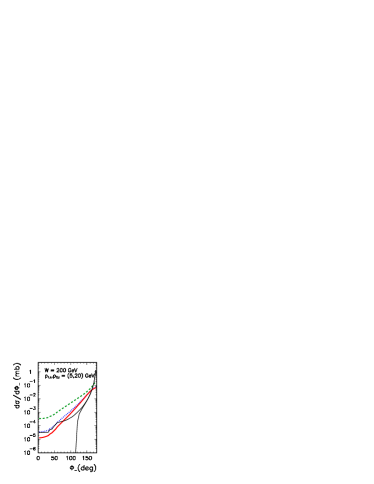
Figure 11: Jet-jet azimuthal correlations $d\sigma/d\phi_{-}$ for the $gg\to gg$ component and different UGDFs as a function of azimuthal angle between the gluonic jets. In this calculation W = 200 GeV and -1 $<y_{1},y_{2}<$ 1, 5 GeV $<p_{1t},p_{2t}<$ 20 GeV. The notation here is the same as in Fig.8.

Figure 12: Cross section for the $gg\to ggg$ component on the $(p_{1,t},p_{2,t})$ plane with the condition of leading jets (partons). The borders of NLO accessible regions are clearly visible.

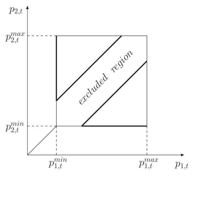
Figure 15: The excluded diagonal region. Shown are also standard cuts on jet transverse momenta.

References

• (1) S.S. Adler et al. (PHENIX collaboration), Phys. Rev. Lett. 97 (2006) 052301;
S.S. Adler et al. (PHENIX collaboration), Phys. Rev. C73 (2006) 054903;
S.S. Adler et al. (PHENIX collaboration), Phys. Rev. Lett. 96 (2006) 222301;
M. Oldenburg et al. (STAR collaboration), Nucl. Phys. A774 (2006) 507.
• (2) S.S. Adler et al. (PHENIX collaborations), Phys. Rev. D74 (2006) 072002.
• (3) P. Levai, G. Fai and G. Papp, Phys. Lett. B634 (2006) 383.
• (4) S. Catani, M. Ciafaloni and F. Hautmann, Nucl. Phys. 366 (1991) 135;
J.C. Collins and R.K. Ellis, Nucl. Phys. B360 (1991) 3.
• (5) J. KwieciΕ„ski, A.D. Martin and A.M. StaΕ›to, Phys. Rev. D56 (1997) 3991;
I.P. Ivanov and N.N. Nikolaev, Phys. Rev. D65 (2002) 054004;
H. Jung and G. Salam, Eur. Phys. Jour. C19 (2002) 351.
• (6) S.P. Baranov and M. SmiΕΎanska, Phys. Rev. D62 (2000) 014012.
• (7) A.V. Lipatov, V.A. Saleev and N.P. Zotov, hep-ph/0112114;
S.P. Baranov, A.V. Lipatov and N.P. Zotov, hep-ph/0302171, Yad. Fiz. 67 (2004) 856.
• (8) M. Łuszczak and A. Szczurek, Phys. Lett. B594 (2004) 291.
• (9) M. Łuszczak and A. Szczurek, Phys. Rev. D73 (2006) 054028.
• (10) A.V. Lipatov and N.P. Zotov, Phys. Rev. D72 (2005) 054002.
• (11) T. Pietrycki and A. Szczurek, hep-ph/0606304, Phys. Rev.D75 (2007) 014023.
• (12) A.V. Lipatov and N.P. Zotov, Eur. Phys. J. C44 (2005) 559;
M. Łuszczak and A. Szczurek, Eur. Phys. J. C46 123 (2006).
• (13) J. KwieciΕ„ski and A. Szczurek, Nucl. Phys. B680 (2004) 164.
• (14) A. Szczurek, Acta Phys. Polon. B34 (2003) 3191.
• (15) M. Czech and A. Szczurek, Phys. Rev. C72 (2005) 015202;
M. Czech and A. Szczurek, J. Phys. G32 (2006) 1253.
• (16) A. Szczurek, N.N. Nikolaev, W. SchΓ€fer and J. Speth, Phys. Lett. B500 (2001) 254.
• (17) A. Leonidov and D. Ostrovsky, Phys. Rev. D62 (2000) 094009.
• (18) A. Szczurek and A. Budzanowski, Phys. Lett. B404 (1998) 141.
• (19) U. D’Alesio and F. Murgia, Phys. Rev. D70 (2004) 074009.
• (20) V.D. Barger and R.J.N. Phillips, β€œCollider physics”, Addison-Wesley Publishing Company, 1987
• (21) F.A. Berends, R. Kleiss, P.De Causmaecker, R. Gastmans, and T.T. Wu, Phys. Lett. B 103 (1981) 124.
• (22) D. Ostrovsky, Phys. Rev. D62 (2000) 054028.
• (23) J. KwieciΕ„ski, Acta Phys. Polon. B33 (2002) 1809;
A. Gawron and J. KwieciΕ„ski, Acta Phys. Polon. B34 (2003) 133;
A. Gawron, J. KwieciΕ„ski and W. Broniowski, Phys. Rev. D68 (2003) 054001.
• (24) J. Bartels, A. Sabio Vera and F. Schwennsen, hep-ph/0608154, JHEP 0611 (2006) 051.
• (25) M.A. Kimber, A.D. Martin and M.G. Ryskin, Eur. Phys. J. C12 (2000) 655;
M.A. Kimber, A.D. Martin and M.G. Ryskin, Phys. Rev. D63 (2001) 114027.
• (26) J. KwieciΕ„ski, A.D. Martin and A.M. StaΕ›to, Phys. Rev. D56 (1997) 3991.
• (27) E.A. Kuraev, L.N. Lipatov and V.S. Fadin, Sov. Phys. JETP 45 (1977) 199;
Ya.Ya. Balitskij and L.N. Lipatov, Sov. J. Nucl. Phys. 28 (1978) 822.
• (28) A.J. Askew, J. KwieciΕ„ski, A.D. Martin and P.J. Sutton, Phys. Rev. D49 (1994) 4402.
• (29) K.J. Eskola, A.V. Leonidov and P.V. Ruuskanen, Nucl. Phys. B481 (1996) 704.
• (30) K. Golec-Biernat and M. WΓΌsthoff, Phys. Rev. D60 (1999) 114023-1.
• (31) D. Kharzeev and E. Levin, Phys. Lett. B523 (2001) 79.
• (32) I.P. Ivanov and N.N. Nikolaev, Phys. Rev. D65 (2002) 054004.
• (33) M. GlΓΌck, E. Reya and A. Vogt, Z. Phys. C67 (1995) 433.
• (34) M. GlΓΌck, E. Reya and A. Vogt, Eur. Phys. J. C5 (1998) 461.
• (35) V.M. Abazov et al. (D0 collaboration), Phys. Rev. Lett. 94 (2005) 221801.