We propose a pedestrian review of the noncommutative standard model in its present state.

dedicated to Alain Connes on the occasion of his 60th birthday

PACS-92: 11.15 Gauge field theories
MSC-91: 81T13 Yang-Mills and other gauge theories

¹ Unité Mixte de Recherche (UMR 6207) du CNRS et des Universités Aix–Marseille 1 et 2 et Sud Toulon–Var, Laboratoire affilié à la FRUMAM (FR 2291)
² also at Universität Kiel, jureit@cpt.univ-mrs.fr
³ also at Université Aix–Marseille 1, krajew@cpt.univ-mrs.fr
⁴ also at Université Aix–Marseille 1, thomas.schucker@gmail.com
⁵ also at Université Aix–Marseille 1, christophstephan@gmx.de

1 Introduction

Understanding the origin of the standard model is currently one of most challenging issues in high energy physics. Indeed, despite its experimental successes, it is fair to say that its structure remains a mystery. Moreover, a better understanding of its structure would provide us with a precious clue towards its possible extensions.

This can be achieved in the framework of noncommutative geometry [1], which is a branch of mathematics pioneered by Alain Connes and aiming at a generalization of geometrical ideas to spaces whose coordinates fail to commute. Motivated by quantum gravity, it is postulated that space-time is a wildly noncommutative manifold at a very high energy. Even if the precise nature of this noncommutative manifold remains unknown, it seems legitimate to assume that at an intermediate scale, say a few orders of magnitude below the Planck scale, the corresponding algebra of coordinates is only a mildly noncommutative algebra of matrix valued functions. When suitably chosen, such a matrix algebra reproduces within the spectral action principle the standard model coupled to gravity [2].

It is worthwhile to notice that this is a bottom-up approach, as opposed to string theory which is a top-down one. Indeed, in noncommutative geometry, one tries to guess the small scale structure of space-time from our present knowledge at the electroweak scale, whereas string theory aims at deriving the standard model directly from the Planck scale physics.

Nevertheless, the physical interpretation of the spectral action principle and its confrontation with present-day experiment still require some contact with the low energy physics. This follows from the standard Wilsonian renormalization group idea. The spectral action provides us with a bare action supposed to be valid at a very high energy of the order of the unification scale. Then, evolving down to the electroweak scale yields the effective low energy physics. This line of thought is very similar to the one adopted in grand unified theories. Indeed, in a certain sense models based on non commutative geometry can be considered as alternatives to grand unification that do not imply proton decay.

Ten years after its discovery [2], the spectral action has recently received new impetus [3, 4, 5] by allowing a Lorentzian signature in the internal space. This mild modification has three consequences.

• The fermion-doubling problem [6] is solved elegantly.

• Majorana masses and consequently the popular seesaw mechanism are allowed for.

• The Majorana masses in turn decouple the Planck mass from the $W$ mass.

Furthermore, Chamseddine, Connes & Marcolli point out an additional constraint on the coupling constants tying the sum of all Yukawa couplings squared to the weak gauge coupling squared. This relation already holds for Euclidean internal spaces [7].

The aim of this paper is to review the present status of the noncommutative standard model in a pedestrian fashion and to illustrate it by numerical examples.

1.1 A Flavour of Noncommutative Geometry

The unification of gravity with the forces of the sub-atomic world, i.e. the electroweak and the strong force is one of the major problems of theoretical physics. The non-gravitational forces are coded in the standard model of particle physics. Taking quantum mechanics as a basis, the standard model is formulated as a quantum field theory, which perturbatively gives extraordinarily precise experimental predictions. From the differential geometric point of view, the total gauge group $G=SU(2)\times U(1)\times SU(3)/(\mathbb{Z}_{2}\times\mathbb{Z}_{3})$ acts on the matter fields being sections in a vector bundle associated to the principal $G$-bundle over the space-time manifold. Since gauge transformations are taken locally, one can thus imagine an ’internal’ space which is attached to each point of the manifold, i.e. reflecting the gauge degrees of freedom. This ’gauge space’ is similar to Kaluza’s point of view.

The geometry of general relativity is different, Riemannian geometry of a curved space-time. By the equivalence principle, gravity arises as a pseudo-force from a general coordinate transformation. General coordinate transformations are diffeomorphisms of the underlying Riemannian manifold, leaving as such the Einstein-Hilbert action invariant. The symmetry acts directly on the manifold $M$ and on its metric.

Would it not be nice to have a picture for the standard model, where symmetries act ’directly’ on an underlying space-time manifold producing the electroweak and strong forces as pseudo-forces by a group of coordinate transformations? Would it not be nice to place gravity and the other forces on the same footing, namely by obtaining all forces as pseudo-forces from some general ’coordinate transformations’ acting on some general ’space-time’? This is what Alain Connes’ noncommutative geometry [1] does for you.

In quantum mechanics, points of the phase space lose their meaning due to Heisenberg’s uncertainty relation, $\Delta x\Delta p\geq\hbar/2$. The commutative algebra of classical observables, i.e. functions on phase space, is made into a noncommutative involution algebra $\mathcal{A}$ due to $[\hat{x}_{i},\hat{p}_{j}]=i\hbar\delta_{ij}$, with the involution $\cdot^{\ast}$ being the Hermitean conjugation. In the relativistic setting, the wavefunctions are square integrable spinors living in the Hilbert space $\mathcal{H}=\mathcal{L}^{2}(\mathcal{S})$. The algebra $\mathcal{A}$ is faithfully represented on $\mathcal{H}$ and the dynamics is given by the Dirac operator $\not{\partial}\in\mathrm{End}(\mathcal{H})$. It is this ‘spectral’ triple $(\mathcal{A},\mathcal{H},\not{\partial})$ (with some additional structure) which describes a Connes’ geometry. A slight shortcoming is the requirement for an Euclidean setting in order to have $\not{\partial}^{\ast}=\not{\partial}$. One assumes that this can be cured by a Wick rotation, but it is still an open question how to implement a Lorentzian signature.

Figure 1: Gravity from commutative geometries

Of particular interest are the commutative spectral triples coming from a compact spin manifold $M$ with $\mathcal{A}=\mathcal{C}^{\infty}(M)$, $\mathcal{H}=\mathcal{L}^{2}(\mathcal{S})$ and $\not{\partial}$. The axioms of the spectral triple are such that there is a one-to-one correspondence between commutative, real spectral triples and Riemannian spin geometries [8]. This reconstruction theorem tells us in particular how to reconstruct the Riemannian metric from the operator algebraic data of the spectral triple. The diffeomorphisms of the manifold have their equivalent in the automorphisms of $\mathcal{A}$ lifted to the spinors and the so called spectral action due to Chamsedinne & Connes [9, 2] reproduces from the eigenvalues of the Dirac operator the Einstein-Hilbert action with positive cosmological constant. One can see the general setting in figure 1.

It is now possible to relax the commutativity of the algebra $\mathcal{A}$. In that sense, a spectral triple $(\mathcal{A},\mathcal{H},\mathcal{D})$ with a noncommutative algebra will still be equivalent to some ’manifold’, now promoted to a space, where points lose their meaning, i.e. a noncommutative space. Connes’ geometry thus does to space-time what quantum mechanics does to phase space. In particular, it is even applicable to discrete spaces, or spaces which have dimension zero. Spectral triples are thus versatile enough to describe spaces, noncommutative or not, discrete or continuous, on an equal footing. For example, to find an algebra $\mathcal{A}_{f}$ whose automorphisms reproduce the gauge symmetries of the standard model, one can define a finite spectral triple, for example with an algebra $\mathcal{A}_{f}$ being a direct sum of matrix algebras. In the case of the standard model, this is $\mathcal{A}_{f}=\mathbb{H}\oplus\mathbb{C}\oplus M_{3}(\mathbb{C})$.

An almost commutative geometry is defined to be the tensor product of two spectral triples, the first one describing a 4-dimensional space-time, and the second is a 0-dimensional discrete spectral triple. A 0-dimensional triple has a finite dimensional algebra $\mathcal{A}_{f}$ and a finite dimensional Hilbert space $\mathcal{H}_{f}$.

Figure 2: Gauge forces from almost commutative geometries

One can show that the spectral action gives the Einstein-Hilbert action together with the bosonic part of the standard model action, in the case where the finite algebra $\mathcal{A}_{f}$ is taken to be a direct sum of matrix algebras, $\mathcal{A}_{f}=\mathbb{H}\oplus\mathbb{C}\oplus M_{3}(\mathbb{C})$. An almost commutative geometry can be viewed as an ordinary (commutative) 4-dimensional space-time with an ’internal’ Kaluza-Klein space attached to each point. The ’fifth’ dimension is a discrete, 0-dimensional space. In figure 2, we tried to visualise this geometric landscape. The automorphisms are the semi-direct product of Diff$(M)$ and the gauge transformations acting on the finite particle content in a certain representation. It is a rather amazing fact that, since everything is formulated in a pure geometrical language, the Higgs fields turns out to be a connection on the ’internal’ space and comes out automatically because of the interplay between the two algebras $\mathcal{C}^{\infty}(M)$ and $\mathcal{A}_{f}$. Probably, this is one of the most appealing features of almost commutative geometry. Indeed, in this framework, the Higgs can be understood as the ’internal’ metric with its dynamics given by the Higgs potential. Calculating the spectral action produces the complete Yang-Mills- Higgs action of the standard model coupled to gravity.

2 The problems of the standard model

It is fair to compare the successes and the shortcomings of the standard model with those of the Balmer-Rydberg formula:

$$\nu=g_{1}n_{1}^{q_{1}}+g_{2}n_{2}^{q_{2}}.$$ (1)

This ansatz contains two discrete parameters $q_{1},q_{2}\in\mathbb{Z}$ and two continuous parameters $g_{1},g_{2}\in\mathbb{R}$, while the $n_{i}\in\mathbb{N}$ are simply labels. These parameters are determined successfully by fitting the ansatz to atomic spectra. As this phenomenological success increased so did the urgency to answer three questions:

• Who ordered the ansatz?

• Does this order imply constraints on the discrete parameter?

• Does this order imply constraints on the continuous parameter?

The three answers came later: quantum mechanics did; yes, $q_{1}=q_{2}=-2$; yes,

$$g_{1}=-g_{2}=\,\frac{m_{e}}{4\pi\hbar^{3}}\,\frac{e^{4}}{(4\pi\epsilon_{0})^{2}}$$ (2)

for the hydrogen atom in agreement with the experimental fit.

Twisting the history of general relativity only slightly, we can start with the purely field theoretic ansatz:

$$S[g]=\int_{M}\,{\textstyle\frac{-1}{16\pi G}}\,[2\Lambda_{c}+R^{q}]\,\hbox{\rm{d}}V,$$ (3)

with one discrete and two continuous parameters, $G$ and $\Lambda_{c}$. The three answers are: Riemannian geometry did; not really, but $q=1$ certainly is the cheapest order; no. Those of you who hate geometry might want to replace the first answer by: Since the meter was officially abolished on October 21st 1983 we must not use any ansatz relying on inertial coordinates and the Einstein-Hilbert ansatz (3) with $q=1$ is the first not to rely on that background.

Now to the non-gravitational forces. The ansatz is an action proposed in bits by Klein, Gordon, Dirac, Weyl, Majorana, Yukawa, Yang, Mills, Brout, Englert and Higgs. Its discrete parameters are a compact, real Lie group $G$, the ‘gauge group’, and three unitary representations on complex Hilbert spaces, $\mathcal{H}_{S}$ for the Higgs scalar, $\mathcal{H}_{L}$ for the left- and $\mathcal{H}_{R}$ for the right-handed Weyl spinors. The continuous parameters are the gauge-invariant couplings whose number increases with the number of simple components in the Lie algebra $\mathfrak{g}$ of $G$ and increases sharply with the number of irreducible components in the representations.

The experimental fit yields the following discrete parameters:

$$G = SU(2)\times U(1)\times SU(3)/(\mathbb{Z}_{2}\times\mathbb{Z}_{3}),$$ (4)

$$\mathcal{H}_{L} = \bigoplus_{1}^{3}\left[(2,{\textstyle\frac{1}{6}},3)\oplus(2,-{\textstyle\frac{1}{2}},1)\right],$$ (6)

$$\mathcal{H}_{R} = \bigoplus_{1}^{3}\left[(1,{\textstyle\frac{2}{3}},3)\oplus(1,-{\textstyle\frac{1}{3}},3)\oplus(1,-1,1)\oplus(1,0,1)\right],$$ (7)

$$\mathcal{H}_{S} = (2,-{\textstyle\frac{1}{2}},1).$$ (8)

Consequently we have the following continuous parameters: three gauge couplings, one quadratic and one quartic Higgs self-coupling, which are traded for the $W$ and the Higgs masses, and a bunch of complex Yukawa couplings, which are traded for the 12 Dirac masses, three Majorana masses and three unitary mixing matrices. We therefore have $3+2+12+3+3\times 4=32$ physically relevant, real, continuous parameters. $4\cdot 3\times 3$ complex Yukawa couplings, which are traded for the 12 Dirac masses and two unitary mixing matrices. Each of these two contains three angles and one phase. Then there is the complex, symmetric $3\times 3$ matrix of Majorana masses containing $2\cdot 6$ real parameters, all physical except for one. We therefore have $3+2+12+2\times 4+11=36$ physically relevant, real, continuous parameters. Today, many of them are known experimentally with good precision [10]. We do not know much about the last eleven, the Majorana mass matrix is constrained weakly by neutrinoless double $\beta$-decay.

Now we face the three questions: where does the complicated ansatz come from, where do its discrete parameters come from, where do its continuous parameters come from?

3 Three answers

3.1 Who ordered the ansatz?

Noncommutative geometry did. Chamsedine & Connes have computed the spectral action for a generic almost commutative geometry. They obtain in addition to the Einstein- Hilbert Lagrangian the following terms:

• the Yang-Mills Lagrangian,

• the Klein-Gordon Lagrangian with the covariant derivative,

• the Higgs potential with its spontaneous symmetry breaking,

• the Dirac Lagrangian for the left- and right-handed Weyl spinors with the covariant derivative,

• the Yukawa couplings.

Note in particular that the first three Lagrangians come with the correct signs relative to the Einstein-Hilbert Lagrangian. In addition there is a term quadratic in the Weyl curvature and a coupling between curvature scalar and the Higgs scalar making the scale-invariant part of the Lagrangian invariant under local dilatations.

We conclude that almost commutative geometry unifies gravity with the other forces in the sense that the latter become pseudo-forces accompanying the former. This is similar to Minkowskian geometry allowing us to interpret the magnetic force as a pseudo-force accompanying the electric force. Or Riemannian geometry allowing, via the equivalence principle, to interpret gravity as a pseudo-force. The definition of a pseudo-force comes with a transformation, a Lorentz transformation for Minkowskian, a general coordinate transformation for Riemannian geometry. The corresponding transformation for noncommutative geometry will be discussed next.

3.2 Constraints on the discrete parameters

There are two ways to extract the gauge group $G$ from the spectral triple.

The first way defines the gauge group to be the unimodular (i.e. of unit determinant) unitary group [11, 5] of the associative algebra, which by the faithful representation immediately acts on the Hilbert space.

The second way follows general relativity whose invariance group is the group of diffeomorphisms of $M$ (general coordinate transformations). In the algebraic formulation this is the group of algebra automorphisms. Indeed Aut$(\mathcal{C}^{\infty}(M))={\rm Diff}(M).$ We still have to lift the diffeomorphisms to the Hilbert space. This lift is double-valued and its image is the semi-direct product of the diffeomorphism group with the local spin group [12]. Also it can be shown perturbatively that in the commutative case the spin lift is unique [13]. In some almost commutative cases, the lift has to be centrally extended in order to remain finitely valued [14]. These extensions are not unique but parameterized by central charges. Let us note that all automorhisms (in the connected component of the identity) of the associative algebras of inner spectral triples are inner while the ones of commutative spectral triples are outer.

Up to possible central $U(1)$s and their central charges, the two approaches coincide.

It follows that all four infinite series in Cartan’s classification of simple Lie algebras are induced from finite spectral triples, but not the five exceptional ones. For example, $G_{2}$ is the Lie algebra of the automorphism group of the non-associative algebra of octonions. This restriction to the gauge groups $U(N)$, $SO(N)$ and $SP(N)$ is reminiscent from open string theories with gauge fields arising from the Chan-Paton factors.

In the even-dimensional case the Hilbert space of the spectral triple is decomposed by the chirality operator into a left- and a right- handed piece, $\mathcal{H}=\mathcal{H}_{L}\oplus\mathcal{H}_{R}$. They define immediately the unitary representation of the ansatz. However not every group representation extends to an algebra representation, only the fundamental ones do. For example take $\mathcal{A}=\mathbb{H}$, the quaternions. Its automorphism group is Aut$(\mathbb{H})=SU(2)/\mathbb{Z}_{2}$, its unitary group $U(\mathcal{A}):=\{u\in\mathcal{A},u^{*}u=uu^{*}=1\}=SU(\mathbb{H})=SU(2)$ is already unimodular. There is only one irreducible representation of the quaternions, $\mathcal{H}=\mathbb{C}^{2}$. All group representations of $SU(2)$ with higher spin do not extend to an algebra representation.

There are other constraints on the fermionic representations coming from the axioms of the spectral triple. They are conveniently captured in Krajewski diagrams which classify all possible finite dimensional spectral triples [15]. They do for spectral triples what the Dynkin and weight diagrams do for groups and representations. Figure 3 shows the Krajewski diagram of the standard model in Lorentzian signature with one generation of fermions including a right-handed neutrino.

Figure 3: Krajewski diagram of the standard model with right-handed neutrino
and Majorana-mass term depicted by the dashed arrow.

Certainly the most restrictive constraint on the discrete parameters concerns the scalar representation. In the Yang-Mills-Higgs ansatz it is an arbitrary input. In the almost commutative setting it is computed from the data of the inner spectral triple.

We find it hard to believe in a coincidence if, despite the mentioned constraints, the standard model fits perfectly into the almost commutative frame. On the other hand, no left-right symmetric model does [16], no grand unified theory does [17] and we have no supersymmetric model that does [18], see figure 4.

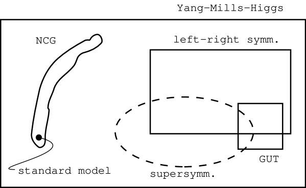
Figure 4: The almost commutative model building kit

Here is the inner triple of the standard model with one generation of fermions including a right-handed neutrino. The algebra has four summands:

$$\mathcal{A}=\mathbb{H}\oplus\mathbb{C}\oplus M_{3}(\mathbb{C})\oplus\mathbb{C}\owns(a,b,c,d),$$ (9)

the Hilbert space is 32-dimensional

$$\mathcal{H}=\mathcal{H}_{L}\oplus\mathcal{H}_{R}\oplus\mathcal{H}_{L}^{c}\oplus\mathcal{H}_{R}^{c},$$ (10)

$$\mathcal{H}_{L}=\mathcal{H}_{L}^{c}\!\! \!\!=\!\! \!\!(\mathbb{C}^{2}\otimes\mathbb{C}^{3})\,\oplus\,(\mathbb{C}^{2}\otimes\mathbb{C}),$$ (11)

$$\mathcal{H}_{R}=\mathcal{H}_{R}^{c}\!\! \!\!=\!\! \!\!(\mathbb{C}\otimes\mathbb{C}^{3})\,\oplus\,(\mathbb{C}\otimes\mathbb{C}^{3})\,\oplus\,(\mathbb{C}\otimes\mathbb{C})\,\oplus\,(\mathbb{C}\otimes\mathbb{C}),$$ (12)

and carries the faithful repesentation

$$\rho(a,b,c):=\pmatrix{\rho_{L}&0&0&0\cr 0&\rho_{R}&0&0\cr 0&0&{\bar{\rho}^{c}_{L}}&0\cr 0&0&0&{\bar{\rho}^{c}_{R}}}$$ (13)

with

$$\rho_{L}(a):=\pmatrix{a\otimes 1_{3}&0\cr 0&a},\ \rho_{R}(b):=\pmatrix{b1_{3}&0&0&0\cr 0&\bar{b}1_{3}&0&0\cr 0&0&b&0\cr 0&0&0&d},$$ (14)

$$\rho^{c}_{L}(c,d):=\pmatrix{1_{2}\otimes c&0\cr 0&\bar{d}1_{2}},\ \rho^{c}_{R}(c,d):=\pmatrix{c&0&0&0\cr 0&c&0&0\cr 0&0&\bar{d}&0\cr 0&0&0&\bar{d}}.$$ (15)

The Dirac operator

$$\tilde{\mathcal{D}}=\pmatrix{0&\mathcal{M}&0&0\cr\mathcal{M}^{*}&0&0&S\cr 0&0&0&\bar{\mathcal{M}}\cr 0&S^{*}&\bar{\mathcal{M}}^{*}&0}$$ (16)

contains Dirac masses

$$\mathcal{M}=\pmatrix{\pmatrix{M_{u}&0\cr 0&0}\otimes 1_{3}+\pmatrix{0&0\cr 0&M_{d}}\otimes 1_{3}&0\cr 0&\pmatrix{M_{\nu}&0\cr 0&0}+\pmatrix{0&0\cr 0&M_{e}}}$$ (17)

and the Majorana mass for the right-handed neutrino,

$$S=\pmatrix{M_{M}&0\cr 0&0}.$$ (18)

For $N$ generations $M_{u},\ M_{d},\ M_{\nu}$ and $M_{e}$ are complex $N\times N$ matrices encoding the Dirac masses and mixings while $M_{M}$ is a complex, symmetric matrix encoding Majorana masses and mixings. For example for the quarks with $N=3$ generations:

$$M_{u}:=\pmatrix{m_{u}&0&0\cr 0&m_{c}&0\cr 0&0&m_{t}}, M_{d}:=C_{KM}\pmatrix{m_{d}&0&0\cr 0&m_{s}&0\cr 0&0&m_{b}},$$ (19)

with the Cabibbo-Kobayashi-Maskawa matrix $C_{KM}$.

This model is conform with the standard formulation of the axiom of Poincaré duality as stated in [1]. It seems to be closely related to the older bi-module approach of the Connes-Lott model [19] which also exhibits two copies of the complex numbers in the algebra. In the original version of the standard model with right-handed Majorana neutrinos Chamseddine, Connes & Marcoli [5] used an alternative spectral triple based on the algebra $\mathcal{A}=\mathbb{H}\oplus\mathbb{C}\oplus M_{3}(\mathbb{C})$. But this spectral triple requires a subtle change in the formulation of the Poincaré duality, i.e. it needs two elements to generate $KO$-homology as a module over $K_{0}$. It should however be noted that right-handed neutrinos that allow for Majorana-masses always fail to fulfil the axiom of orientability [20] since the representation of the algebra does not allow to construct a Hochschild-cycle reproducing the chirality operator. For this reason we have drawn the arrows connected to the right-handed neutrinos with broken lines in the Krajewski diagram.

3.3 Constraints on the continuous parameters

3.3.1 The dimensionless parameters

The spectral action counts the number of eigenvalues of the Dirac operator whose absolute values are less than the energy cut-off $\Lambda$. On the input side its continuous parameters are: this cut- off, three positive parameters in the cut-off functions and the parameters of the inner Dirac operator, i.e. fermion masses and mixing angles. On the output side we have: the cosmological constant, Newton’s constant, the gauge and the Higgs couplings. Therefore there are constraints, which for the standard model with $N$ generations and three colours read:

$$\,\frac{5}{3}\,g_{1}^{2}=g_{2}^{2}=g_{3}^{2}=\,\frac{3}{N}\,\frac{Y_{2}^{2}}{H}\,\frac{\lambda}{24}\,=\,\frac{3}{4N}\,Y_{2}\,.$$ (20)

Here $Y_{2}$ is the sum of all Yukawa couplings $g_{f}$ squared, $H$ is the sum of all Yukawa couplings raised to the fourth power. Our normalisations are: $m_{f}=\sqrt{2}\,(g_{f}/g_{2})\,m_{W},$ $(1/2)\,(\partial\varphi)^{2}+(\lambda/24)\,\varphi^{4}$. If we define the gauge group by lifted automorphisms rather than unimodular unitairies, then we get an ambiguity parameterized by the central charges. This ambiguity leaves the $U(1)$ coupling $g_{1}$ unconstrained and therefore kills the first of the four constraints (20).

Note that the noncommutative constraints (20) are different from Veltman’s condition [21], which in our normalisation reads:

$${\textstyle\frac{3}{4}}g_{2}^{2}+{\textstyle\frac{1}{4}}g_{1}^{2}+{\textstyle\frac{1}{3}}\lambda-2g_{t}^{2}=0.$$ (21)

Of course the constraints (20) are not stable under the renormalisation group flow and as in grand unified theories we can only interpret them at an extremely high unification energy $\Lambda$. But in order to compute the evolution of the couplings between our energies and $\Lambda$ we must resort to the daring hypothesis of the big desert, popular since grand unification. It says: above presently explored energies and up to $\Lambda$ no more new particle, no more new forces exist, with the exception of the Higgs, and that all couplings evolve without leaving the perturbative domain. In particular the Higgs self-coupling $\lambda$ must remain positif. In grand unified theories one believes that new particles exist with masses of the order of $\Lambda$, the leptoquarks. They mediate proton decay and stabilize the constraints between the gauge couplings by a bigger group. In the noncommutative approach we believe that at the energy $\Lambda$ the noncommutative character of space-time ceases to be negligible. The ensuing uncertainty relation in space-time might cure the short distance divergencies and thereby stabilize the constraints. Indeed Grosse & Wulkenhaar have an example of a scalar field theory on a noncommutative space-time with vanishing $\beta$-function [22].

Let us now use the one-loop $\beta$-functions of the standard model with $N=3$ generations to evolve the constraints (20) from $E=\Lambda$ down to our energies $E=m_{Z}$. We set: $t:=\ln(E/m_{Z}),\quad\hbox{\rm{d}}g/\hbox{\rm{d}}t=:\beta_{g},\quad\kappa:=(4\pi)^{-2}.$ We will neglect all fermion masses below the top mass and also neglect threshold effects. We admit a Dirac mass $m_{D}$ for the $\tau$ neutrino induced by spontaneous symmetry breaking and take this mass of the order of the top mass. We also admit a Majorana mass $m_{M}$ for the right-handed $\tau$ neutrino. Since this mass is gauge invariant it is natural to take it of the order of $\Lambda$. Then we get two physical masses for the $\tau$ neutrino: one is tiny, $m_{\ell}\sim m_{D}^{2}/m_{M}$, the other is huge, $m_{r}\sim m_{M}.$ This is the popular seesaw mechanism [23]. The renormalisation of these masses is well-known [24]. By the Appelquist-Carazzone decoupling theorem [25] we distinguish two energy domains: $E>m_{M}$ and $E<m_{M}$. In the latter, the Yukawa coupling of the $\tau$ neutrino drops out of the $\beta$-functions and is replaced by an effective coupling

$$k=2\,\frac{g_{\nu}^{2}}{m_{M}}\,,\quad{\rm at\ }E=m_{M}.$$ (22)

At high energies, $E>m_{M}$, the $\beta$-functions are [26, 27]:

$$\beta_{g_{i}} = \kappa b_{i}g_{i}^{3},\quad b_{i}={\textstyle\left(\frac{20}{9}N+\frac{1}{6},-\frac{22}{3}+\frac{4}{3}N+\frac{1}{6},-11+\frac{4}{3}N\right)},$$ (23)

$$\beta_{t} = \kappa\left[-\sum_{i}c_{i}^{u}g_{i}^{2}+Y_{2}+\,\frac{3}{2}\,g_{t}^{2}\,\right]g_{t},$$ (25)

$$\beta_{\nu} = \kappa\left[-\sum_{i}c_{i}^{\nu}g_{i}^{2}+Y_{2}+\,\frac{3}{2}\,g_{\nu}^{2}\,\right]g_{\nu},$$ (26)

$$\beta_{\lambda} = \kappa\left[\,\frac{9}{4}\,\left(g_{1}^{4}+2g_{1}^{2}g_{2}^{2}+3g_{2}^{4}\right)-\left(3g_{1}^{2}+9g_{2}^{2}\right)\lambda+4Y_{2}\lambda-12H+4\lambda^{2}\right],$$ (27)

with

$$c_{i}^{t}=\left({\textstyle\frac{17}{12}},{\textstyle\frac{9}{4}},8\right), c_{i}^{\nu}=\left({\textstyle\frac{3}{4}},{\textstyle\frac{9}{4}},0\right),$$ (28)

$$Y_{2}=3g_{t}^{2}+g_{\nu}^{2}, H=3g_{t}^{4}+g_{\nu}^{4}.$$ (29)

At low energies, $E<m_{M}$, the $\beta$-functions are the same except that $Y_{2}=3g_{t}^{2}$, $H=3g_{t}^{4}$ and that $\beta_{\nu}$ is replaced [24] by:

$$\beta_{k}=\kappa\left[-3g_{2}^{2}+\,\frac{3}{2}\,-\sum_{i}c_{i}^{\nu}g_{i}^{2}+Y_{2}+\,\frac{2}{3}\,\lambda+2Y_{2}\,\right]k.$$ (30)

We suppose that all couplings (other than $g_{\nu}$ and $k$) are continuous at $E=m_{M}$, no threshold effects. The three gauge couplings decouple from the other equations and have identical evolutions in both energy domains:

$$g_{i}(t)=g_{i0}/\sqrt{1-2\kappa b_{i}g_{i0}^{2}t}.$$ (31)

The initial conditions are taken from experiment [10]:

$$g_{10}=0.3575,\quad g_{20}=0.6514,\quad g_{30}=1.221.$$ (32)

In a first run we leave $g_{1}$ unconstrained. Then the unification scale $\Lambda$ is the solution of $g_{2}(\ln(\Lambda/m_{Z}))=g_{3}(\ln(\Lambda/m_{Z}))$,

$$\Lambda=m_{Z}\exp\frac{g_{20}^{-2}-g_{30}^{-2}}{2\kappa(b_{2}-b_{3})}\,=\,1.1\times 10^{17}\ {\rm GeV},$$ (33)

and is independent of the number of generations.

Then we choose $g_{\nu}=Rg_{t}$ at $E=\Lambda$ and $m_{M}$ and solve numerically the evolution equations for $\lambda,\ g_{t},\ g_{\nu}$ and $k$ with initial conditions at $E=\Lambda$ from the noncommutative constraints (20):

$$g_{2}^{2}=\,\frac{3+R^{2}}{3+R^{4}}\,\frac{\lambda}{24}\,=\,\frac{3+R^{2}}{4}\,g_{t}^{2}\,.$$ (34)

We note that these constraints imply that all couplings remain perturbative and at our energies we obtain the pole masses of the Higgs, the top and the light neutrino:

$$m_{H}^{2}=\,\frac{4}{3}\,\frac{\lambda(m_{H})}{g_{2}(m_{Z})^{2}}\,m_{W}^{2},\quad m_{t}=\sqrt{2}\,\frac{g_{t}(m_{t})}{g_{2}(m_{t})}\,m_{W},\quad m_{\ell}=\,\frac{k(m_{Z})}{g_{2}(m_{Z})^{2}}\,m_{W}^{2}.$$ (35)

A few numerical results are collected in table 1.

$g_{\nu}/g_{t}|_{\Lambda}$	0	1.16	1.16	1.2	1.2	1.3	1.3	1.4	1.4
$m_{M}$ [GeV]	*	$2\cdot 10^{13}$	$10^{14}$	$2\cdot 10^{13}$	$10^{14}$	$3\cdot 10^{13}$	$10^{14}$	$3\cdot 10^{13}$	$10^{14}$
$m_{t}$ [GeV]	186.3	173.3	173.6	172.5	172.8	170.5	170.7	168.4	168.6
$m_{H}$ [GeV]	188.4	170.5	170.8	169.7	170.0	167.7	168.0	165.8	166.1
$m_{\ell}$ [ eV]	0	0.29	0.06	0.30	0.06	0.23	0.07	0.25	0.08

Table 1: The top, Higgs and neutrino masses as a function of $R$ and of the Majorana mass for the unification scale $\Lambda=1.1\times 10^{17}$ GeV

Note that the Higgs mass is not very sensitive to the three input parameters, $\Lambda,\ m_{M},$ and $R=g_{\nu}(\Lambda)/g_{t}(\Lambda)$ as long as they vary in a range reproducing senible masses for the top and the light neutrino, today $m_{t}=170.9\,\pm 2.6$ GeV and $0.05\ {\rm eV}\ <\ m_{\ell}\ <\ 0.3$ eV. Then we have for the Higgs mass

$$m_{H}=168.3\pm 2.5\ {\rm GeV}.$$ (36)

In a second run we use the constraint on the Abelian coupling $\,\frac{5}{3}\,g_{1}^{2}=g_{2}^{2}$ to compute the unification scale:

$$\Lambda=m_{Z}\exp\frac{g_{20}^{-2}-(3/5)g_{30}^{-2}}{2\kappa(b_{2}-(3/5)b_{1})}\,=\,9.8\times 10^{12}\ {\rm GeV}.$$ (37)

Note that the third constraint $\,\frac{5}{3}\,g_{1}^{2}=g_{3}^{2}$ yields an intermediate unification scale, $\Lambda=2.4\times 10^{14}\ {\rm GeV}.$ Again we give a few numerical results, table 2.

$g_{\nu}/g_{t}|_{\Lambda}$	0	0.95	1	1.1	1.2
$m_{t}$ [GeV]	183.4	173.3	172.3	170.3	168.1
$m_{H}$ [GeV]	188.5	174.9	173.8	171.9	170.2
$m_{\ell}$ [ eV]	0	0.53	0.57	0.67	0.77

Table 2: The top, Higgs and neutrino masses as a function of $R$ for the Majorana mass and the unification scale $m_{M}=\Lambda=9.8\times 10^{12}$ GeV

Here the upper bound for the light neutrino mass cannot be met strictly with $m_{M}<\Lambda$. This does not worry us because that bound derives from cosmological hypotheses. Honouring the constraints for all three gauge couplings then yields the combined range for the Higgs mass,

$$m_{H}=168.3^{+6.6}_{-2.5}\ {\rm GeV}.$$ (38)

3.3.2 Constraints on the dimensionful parameters

The spectral action also produces constraints between the quadratic Higgs coupling, the Planck mass, $m_{P}^{2}=1/G$, and the cosmological constant in terms of the cut-off $\Lambda$ and of the three moments, $f_{0},f_{2},f_{4}$, of the cut-off function. A step function for example has $2f_{0}=f_{2}=f_{4}$. Trading the quadratic Higgs coupling for the $W$ mass, these constraints read:

$$m_{W}^{2}=\frac{45}{4\cdot 96}\frac{(3m_{t}^{2}+m_{\nu}^{2})^{2}}{3m_{t}^{4}+m_{\nu}^{4}}\left[\frac{f_{2}}{f_{4}}\,\Lambda^{2}-\frac{m_{\nu}^{2}}{3m_{t}^{2}+m_{\nu}^{2}}\,m_{M}^{2}\right]\sim\frac{45}{96}\left[\frac{f_{2}}{f_{4}}\,\Lambda^{2}-\frac{1}{4}\,m_{M}^{2}\right],$$ (39)

$$m_{P}^{2} = \frac{1}{3\pi}\left[\left(96-4\,\frac{(3m_{t}^{2}+m_{\nu}^{2})^{2}}{3m_{t}^{4}+m_{\nu}^{4}}\right)f_{2}\Lambda^{2}+2\left(2\,\frac{m_{\nu}^{2}(3m_{t}^{2}+m_{\nu}^{2})}{3m_{t}^{4}+m_{\nu}^{4}}-1\right)f_{4}m_{M}^{2}\right]$$ (40)

$$\sim \frac{1}{3\pi}\left[80f_{2}\Lambda^{2}+2f_{4}m_{M}^{2}\right],$$ (42)

$$\Lambda_{c} \sim \frac{1}{\pi m_{P}^{2}}[(96\cdot 2f_{0}-16f_{2}2/f_{4})\Lambda^{4}+f_{4}m_{M}^{4}+4f_{2}\Lambda^{2}m_{M}^{2}].$$ (43)

We have taken three generations, i.e. a 96-dimensional inner Hilbert space, we only kept the Yukawa couplings of the top quark and of the $\tau$ neutrino, and one single Majorana mass in the third generation. The experts still do not agree whether the renormalisation group flow of the quadratic Higgs coupling is logarithmic or quadratic in the energy $E$. Nobody knows how Newton’s and the cosmological constants depend on energy. Therefore we cannot put the above constraints to test. It is however reassuring that, thanks to the seesaw mechanism, a $W$ mass much smaller than the Planck mass is easily obtained. On the other hand it is difficult to produce a small cosmological constant.

4 Is the standard model special?

4.1 Privileged solutions of the constraints on the discrete parameters

Despite all constraints, there is still an infinite number of Yang- Mills-Higgs-Dirac-Yukawa models that can be derived from gravity using almost commutative geometry. The exploration of this special class is highly non-trivial and starts with Krajewski diagrams. Of course one would like to show that the standard model has a privileged position in the class as indicated in figure 4.

At present there are two approaches in this direction.

The first by Chamseddine, Connes & Marcolli [5] starts from a left-right symmetric algebra. This algebra admits a privileged bi-module which is identical to the fermionic Hilbert space of the standard model. The algebra of the standard model is a maximal subalgebra of the left-right symmetric one and the inner Dirac operator is almost the maximal operator satisfying the axioms of a spectral triple. The number of colours and the number of generations remain unexplained in this approach.

The second approach again has nothing to say about the number of colours and generations. It is a more opportunistic approach and copies what grand unified theories [28] did in the frame of Yang-Mills-Higgs-Dirac-Yukawa theories. There, the idea was to cut down on the number of possible models with a ‘shopping’ list of requirements: one wants

• the gauge group to be simple,

• the fermion representation irreducible,

• the fermion representation complex under the gauge group,

• the fermion representation to be free of Yang-Mills anomalies,

• the model to contain the standard model.

The motivations for these requirements were of heteroclitic origin, mathematical simplicity, the wish to be able to distinguish particle from anti-particles, consistency of the ensuing quantum field theory, consistency with the phenomenology. Two examples with gauge group $SO(10)$ and $E_{6}$ and accounting for one generation of fermions were on the market. On the other hand at that time $F_{4}$ was banned because it does not have complex representations.

Coming back to Connes’ noncommutative model building kit, we remark that the spectral triple of the standard model with one generation of fermions and a massless neutrino is irreducible. It has another remarkable property concerning its built-in spontaneous symmetry breaking: it allows a vacuum giving different masses to the two quarks although they sit in an isospin doublet. Indeed, in the majority of noncommutative models the spontaneous symmetry breaking gives degenerate masses to fermions in irreducible group representations. We say that those models are “ dynamically degenerate” because there are other mass degeneracies coming from the kinematics, i.e the axioms of the spectral triple without using the spectral action and its induced spontaneous symmetry breaking. These “kinematical” degeneracies are always protected by a gauge group, which we call “colour group” because in the standard model this group is the colour group.

For years we have been looking for viable noncommutative models other than the standard model, without success. We therefore started to scan the Krajewski diagrams with the following shopping list. We want:

• the spectral triple to be irreducible,

• the fermion representation to be complex under the little group in every irreducible component,

• possible massless fermions to transform trivially under the little group,

• the fermion representation to be free of Yang-Mills and mixed gravitational Yang-Mills anomalies,

• the spectral triple to have no dynamical degeneracy and the colour group of every kinematical degeneracy to remain unbroken.

The first step is to get the list of irreducible Krajewski diagrams (letter-changing arrows only) [29]. In the case of an inner spectral triple of Euclidean signature, we have no such diagram for a simple algebra, one diagram for an algebra with two simple summands, 30 diagrams for three summands, 22 diagrams for four summands, altogether 53 irreducible diagrams for algebras with up to four simple summands. The situation simplifies when we go to the Lorentzian signature where we remain with only 7 diagrams for up to four summands. These numbers are summarized in table 3.

#(summands)	Eulidean	Lorentzian
1	$\ \ 0$	0
2	$\ \ 1$	0
3	30	0
4	22	7
$\!\!\!\!\!\!\leq 4$	53	7

Table 3: The number of irreducible Krajewski diagrams for algebras with up to 4 simple summands and inner spaces with Eucidean and Lorentzian signatures, letter-changing arrows only

The second step is to scan all models derived from the irreducible Krajewski diagrams with respect to our shopping list. In both signatures we remain with the following models: The standard model with one generation of fermions, an arbitrary number of colours $C\geq 2$ and a massless neutrino:

$$\frac{SU(2)\times U(1)\times SU(C)}{\mathbb{Z}_{2}\times\mathbb{Z}_{C}} \longrightarrow \frac{U(1)\times SU(C)}{\mathbb{Z}_{C}}$$ (44)

For even $C$ the $\mathbb{Z}_{2}$ factor is missing. We also have three possible submodels with identical fermion content, but with $SU(2)$ replaced by $SO(2)$, no $W$-bosons, or with $SU(C)$ replaced by $SO(C)$ or $USp(C/2)$, $C$ even, less gluons. There is one more possible model, the elctro-strong model:

$${U(1)\times SU(C)} \longrightarrow {U(1)\times SU(C)}$$ (45)

The fermionic content is ${\underline{C}}\oplus{\underline{1}}$, one quark and one charged lepton. The two electric charges are arbitrary but vectorlike. The model has no scalar and no symmetry breaking.

For those of you who think that our shopping list is unreasonably restrictive already in the frame of Yang-Mills-Higgs-Dirac-Yukawa models, here is a large class of such models satisfying our shopping list: Take any group that has complex representations (like $E_{6}$) and take any irreducible, complex, unitary representation of this group. Put the left- and right-handed fermions in two copies of this representation, choose the Hilbert space for scalars 0-dimensional and a gauge-invariant mass for all fermions.

4.2 Beyond the standard model

For many years we have been trying to construct models from noncommutative geometry that go beyond the standard model [30] and we failed to come up with anything physical if it was not to add more generations and right-handed neutrinos to the standard model.

The noncommutative constraints on the continuous parameters of the standard model with $N=4$ generations fail to be compatible with the hypothesis of the big desert [31].

Since a computer program [32] was written to list the irreducible Krajewski diagrams for algebras with more than three summands we do have a genuine extension of the standard model satisfying all physical desirata. It comes from an algebra with six summands [33] and is identical to the standard model with two additional leptons $A^{--}$ and $C^{++}$ whose electric charge is two in units of the electron charge. These new leptons couple neither to the charged gauge bosons, nor to the Higgs scalar. Their hypercharges are vector-like, so that they do not contribute to the electroweak gauge anomalies. Their masses are gauge-invariant and they constitute viable candidates for cold dark matter [34].

Also, by trial and error, two more models could be found recently [35, 36]. The first model is based on an algebra with six summands and adds to the standard model a lepton-like, weakly charged, left-handed doublet and two right-handed hypercharge singlets. These four particles are each colour-doublets under a new $SU(2)_{c}$ colour group. They participate in the Higgs mechanism and the noncommutative constraints require masses to be around $75$ GeV. Since they have a non-Abelian colour group one expects a macroscopic confinement [37] with a confinement radius of $\sim 10^{-5}$ cm. Although these particles have electro-magnetic charge after symmetry breaking it is not yet clear whether they could have been detected in existing experiments.

The second model adds to the standard model three generations of vectorlike doublets with weak and hypercharge. After symmetry breaking one particle of each doublet becomes electrically neutral while its partner acquires a positive or a negative electro-magnetic charge (depending on the choice of the hypercharge). The particles, like the $AC$ leptons, do not couple to the Higgs boson and should have masses of the order of $\sim 10^{3}$ TeV. Due to differing self-interaction terms with the photon and the Z-boson the neutral particle will be slightly lighter than the charged particle and is therefore the stable state [38]. Together with its neutrino-like cross section the neutral particle constitutes an interesting dark matter candidate [39].

Another interesting aspect of the models presented in [35] and [36] is that they naturally exhibit gauge unification at around $10^{13}$ GeV. This should be seen in contrast to the $AC$ model which only aggravates the situation of the lacking unification in the standard model.

5 Conclusions

There are two clear-cut achievements of noncommutative geometry in particle physics:

• Connes’ derivation of the Yang-Mills-Higgs-Dirac-Yukawa ansatz from the Einstein-Hilbert action,

• the fact that this unification of all fundamental forces allows to compute correctly the representation content of the Higgs scalar (i.e. one weak isospin doublet, colour singlet with hyper-charge one half) from the experimentally measured representation content of the fermions.

The other clear achievements are restrictions on the gauge groups, severe restrictions on the fermion representations and their compatibility with experiment.

Finally there are constraints on the top and Higgs masses. They do rely on the hypothesis of the big desert. Nevertheless we look forward to the Tevatron and LHC verdict.

To our taste the comparison of these achievements with the explanation of the Balmer-Rydberg formula by quantum mechanics is fair. We think of the early Bohr model, which already did this job. The Bohr model certainly had its shortcomings and did not pretend to be the last word, but it pointed in the right direction. So in what direction is noncommutative geometry pointing? For us it holds the promise to clean up quantum field theory and thereby including quantum gravity. Apparently this motivation for noncommutative geometry already goes back to Heisenberg [40].

References

- [1] A. Connes, Noncommutative Geometry, Academic Press (1994) and http://www.alainconnes.org/
- [2] A. Chamseddine & A. Connes, The spectral action principle, hep- th/9606001, Comm. Math. Phys. 182 (1996) 155
- [3] A. Connes, Noncommutative geometry and the standard model with neutrino mixing, hep-th/0608226, JHEP 0611 (2006) 081
- [4] J. Barrett, A Lorentzian version of the non-commutative geometry of the standard model of particle physics, hep-th/0608221, J. Math. Phys. 48 (2007)012303
- [5] A. Chamseddine, A. Connes & M. Marcolli, Gravity and the standard model with neutrino mixing, hep-th/0610241
-
[6]
F. Lizzi, G. Mangano, G. Miele & G. Sparano,
Fermion Hilbert space and fermion doubling in the noncommutative geometry approach to gauge theories,
hep-th/9610035,
Phys. Rev. D55 (1997) 6357
J. M. Gracia-Bondía, B. Iochum & T. Schücker, The standard model in noncommutative geometry and fermion doubling, hep-th/9709145, Phys. Lett. B414 (1998) 123 - [7] T. Thumstädter, Prameteruntersuchungen an Dirac-Modellen, PhD- thesis, Universität Mannheim (2003)
- [8] A. Rennie & J. Várilly, Reconstruction of manifolds in noncommutative geometry, math.OA/0610418
- [9] A. Connes, Gravity coupled with matter and the foundation of noncommutative geometry, hep-th/9603053, Comm. Math. Phys. 155 (1996) 109
- [10] The Particle Data Group, Review of Particle Physics, J. Phys. G33 (2006) 1 and http://pdg.lbl.gov
- [11] A. Connes, Noncommutative geometry and reality, J. Math. Phys. 36 (1995) 6194
- [12] T. Schücker, Spin groups and almost commutative geometry, hep-th/0007047
- [13] B. Iochum & T. Schücker, Diffeomorphisms and orthonormal frames, hep-th/0406213, J. Geom. Phys. 56 (2006) 1496
- [14] S. Lazzarini & T. Schücker, A farewell to unimodularity, hep-th/0104038, Phys. Lett. B510 (2001) 277
-
[15]
M. Paschke & A. Sitarz, Discrete spectral triples and
their symmetries, q-alg/9612029, J. Math. Phys. 39 (1998) 6191
T. Krajewski, Classification of finite spectral triples, hep-th/ 9701081, J. Geom. Phys. 28 (1998) 1 - [16] B. Iochum & T. Schücker, A left-right symmetric model à la Connes-Lott, hep-th/9401048, Lett. Math. Phys. 32 (1994) 153
-
[17]
B. Iochum, D. Kastler & T. Schücker, Fuzzy mass relations for the Higgs, hep-th/9506044, J.
Math. Phys. 36 (1995) 6232
F. Lizzi, G. Mangano, G. Miele & G. Sparano, Constraints on unified gauge theories from noncommutative geometry, hep-th/9603095, Mod. Phys. Lett. A11 (1996) 2561 - [18] W. Kalau & M. Walze, Supersymmetry and noncommutative geometry, hep-th/9604146, J. Geom. Phys. 22 (1997) 77
- [19] A. Connes & J. Lott, Particle models and noncommutative geometry, Nucl. Phys. Proc. Suppl. 18B, (1991) 29-47
- [20] C. Stephan, Almost-commutative geometry, massive neutrinos and the orientability axiom in KO-dimension 6, hep-th/0610097 (2006)
- [21] M. Veltman, The infrared-ultraviolet connection, Acta Phys. Polon. 12 (1981) 437
- [22] H. Grosse & R. Wulkenhaar, The -function in duality-covariant noncommutative theory, hep-th/0402093, Eur. Phys. J. C35 (2004) 277
-
[23]
M. Gell-Mann, P. Ramond & Richard Slansky,
Complex spinors and unified theories,
in Supergravity, P. van Nieuwenhuizen & D. Z. Freedman (eds.), North Holland (1979)
T. Yanagida, Horizontal symmetry and masses of neutrinos, In Proceedings of the Workshop on the Baryon Number of the Universe and Unified Theories, Tsukuba, Japan, (1979) 13, also in Paris 2004, Seesaw 25, 261
R. N. Mohapatra & G. Senjanovic, Neutrino mass and spontaneous parity violation, Phys. Rev. Lett. 44 (1980) 912 -
[24]
K. S. Babu, C. N. Leung & J. T. Pantaleone,
Renormalization of the neutrino mass operator,
hep-ph/9309223,
Phys. Lett. B319 (1993) 191
J. A. Casas, V. Di Clemente, A. Ibarra & M. Quiros, Massive neutrinos and the Higgs mass window, hep-ph/9904295, Phys. Rev. D62 (2000) 053005
S. Antusch, J. Kersten, M. Lindner & M. Ratz, Neutrino mass matrix running for nondegenerate seesaw scales, hep-ph/0203233, Phys. Lett. B538 (2002) 87
S. Antusch, J. Kersten, M. Lindner, M. Ratz & M. A. Schmidt, Running neutrino mass parameters in see-saw scenarios, hep-ph/ 0501272, JHEP 0503 (2005) 024 - [25] T. Appelquist & J. Carazzone, Infrared singularities and massive fields, Phys. Rev. D11 (1975) 2856
- [26] M. E. Machacek & M. T. Vaughn, Two loop renormalization group equations in a general quantum field theory. 1. Wave function renormalization, Nucl. Phys. B222 (1983) 83, 2. Yukawa couplings, Nucl. Phys. B236 (1984) 221, 3. Scalar quartic couplings, Nucl. Phys. B249 (1985) 70
- [27] C. Ford, D. R. T. Jones, P. W. Stephenson & M. B. Einhorn, The effective potential and the renormalisation group, Nucl. Phys. B395 (1993) 17
- [28] H. Georgi & S.L. Glashow, Unity of all elementary-particle forces, Phys. Rev. Lett. 32 (1974) 438
-
[29]
B. Iochum, T. Schücker & C. Stephan, On a classification of
irreducible almost commutative geometries, hep-th/0312276,
J. Math. Phys. 45 (2004) 5003
J.-H. Jureit & C. Stephan, On a classification of irreducible almost commutative geometries, a second helping, hep-th/ 0501134, J. Math. Phys. 46 (2005) 043512
T. Schücker, Krajewski diagrams and spin lifts, hep-th/0501181
J.-H. Jureit, T. Schücker & C. Stephan, On a classification of irreducible almost commutative geometries III, hep-th/0503190, J. Math. Phys. 46 (2005) 072303
J.-H. Jureit & C. Stephan, On a classification of irreducible almost commutative geometries IV, hep-th/0610040 -
[30]
B. Iochum & T. Schücker, Yang-Mills-Higgs versus Connes-Lott,
hep-th/9501142, Comm. Math. Phys. 178 (1996) 1
I. Pris & T. Schücker, Non-commutative geometry beyond the standard model, hep-th/9604115, J. Math. Phys. 38 (1997) 2255
I. Pris & T. Krajewski, Towards a gauge boson in noncommutative geometry, hep-th/9607005, Lett. Math. Phys. 39 (1997) 187
M. Paschke, F. Scheck & A. Sitarz, Can (noncommutative) geometry accommodate leptoquarks? hep-th/9709009, Phys. Rev. D59 (1999) 035003
T. Schücker & S. ZouZou, Spectral action beyond the standard model, hep-th/0109124 - [31] M. Knecht & T. Schücker, Spectral action and big desert, hep- ph/0605166, Phys. Lett. B640 (2006) 272
- [32] J.-H. Jureit & C. Stephan, Finding the standard model of particle physics, a combinatorial problem, hep-th/0503085
- [33] C. Stephan, Almost-commutative geometries beyond the standard model, hep-th/ 0509213
-
[34]
D. Fargion, M. Khlopov & C. Stephan,
Cold dark matter by heavy double charged leptons?,
astro-ph/0511789, Class. Quant. Grav. 23 (2006) 7305
M. Y. Khlopov & C. Stephan, Composite dark matter with invisible light from almost-commutative geometry, astro-ph/0603187 - [35] C. Stephan, Almost-commutative geometries beyond the standard model II: New colours, to appear
- [36] R. Squellari & C. Stephan, Almost-commutative geometries beyond the standard model III: Vector doublets, to appear
- [37] L.B. Okun, Theta particles, Nucl. Phys. B 173 (1980) 1
- [38] S. Thomas & J.D. Wells, Phenomenology of massive vectorlike doublet leptons, Phys. Rev. Lett. 81 (1998) 1
- [39] K. Griest & M. Kamionkowski, Unitarity limits on the mass and radius of dark matter particles, Phys. Rev. Lett. 64 (1990) 615
- [40] R. Jackiw, Physical instances of noncommuting coordinates, hep-th/0110057, Nucl. Phys. Proc. Suppl. 108 (2002) 30, Phys. Part. Nucl. 33 (2002) S6, Lect. Notes Phys. 616 (2003) 294