The Glassy Wormlike Chain

Abstract

We introduce a new model for the dynamics of a wormlike chain in an environment that gives rise to a rough free energy landscape, which we baptise the glassy wormlike chain. It is obtained from the common wormlike chain by an exponential stretching of the relaxation spectrum of its long-wavelength eigenmodes, controlled by a single parameter ${\cal E}$. Predictions for pertinent observables such as the dynamic structure factor and the microrheological susceptibility exhibit the characteristics of soft glassy rheology and compare favourably with experimental data for reconstituted cytoskeletal networks and live cells. We speculate about the possible microscopic origin of the stretching, implications for the nonlinear rheology, and the potential physiological significance of our results.

klaus.kroy@itp.uni-leipzig.de

1 Introduction

Studies of in vitro polymerised networks and solutions of the biopolymers that constitute the cytoskeleton have provided many important insights into the molecular origin of the fascinating mechanical properties of cells and tissues [1]. Cell rheological data [2, 3] are therefore often interpreted in terms of viscoelastic models developed for in vitro reconstituted cytoskeletal networks [4, 5, 6, 7, 8], and the inferred parameters have been suggested as pertinent indices for clinical diagnosis [9]. Also current rheological models for the active processes in the cytoskeleton are rooted in this viscoelastic paradigm [10, 11, 12]. In contrast, microrheological measurements [13] have revealed that cells obey the highly universal and comparatively featureless pattern of soft glassy rheology [14], ubiquitous in soft condensed matter [15]. Integrating these competing paradigms into a unified framework has become a major challenge in cell biophysics [16, 17, 18]. Recent experiments with highly purified reconstituted actin solutions have revealed strong signatures of a glass transition that might hold the key to a resolution of the dilemma [19]. The glass transition manifests itself in a strong stretching of the relaxation spectrum, so that experiments probing the mechanical properties at a fixed time scale detect a sharp transition from fluid-like to solid-like behaviour as a function of various control parameters. In the following, we introduce a new model motivated by this observation, which is able to explain the apparently conflicting phenomenology on a common basis. We call it the glassy wormlike chain (GWLC), because its essence is an exponential stretching of the relaxation spectrum of the wormlike chain (WLC) model, which is the minimal model of a semiflexible polymer. The stretching is quantified by a single parameter ${\cal E}$, the stretching parameter, which can be thought of as a characteristic scale for the free energy barriers retarding the relaxation of the test chain’s long wavelength eigenmodes. The characteristics of soft glassy rheology naturally ensue, including the widely reported small apparent power-law exponents in the frequency-dependence of the microrheological moduli [13, 14, 16, 17], or the so-called “noise temperatures”. Despite of the striking simplicity of the model (${\cal E}$ is the only free parameter), which is in stark contrast to prevailing viscoelastic models for cytosekeletal networks in vitro and in vivo [4, 20], its predictions compare favourably with experimental data for live cells and reconstituted cytoskeletal networks. In particular, the logarithmic tails of the dynamic structure factor obtained by high-precision quasi-elastic light scattering from F-actin solutions at low temperatures and high concentrations [19] provide very direct evidence for the postulated exponential stretching. While a microscopic derivation of ${\cal E}$ remains so far elusive, we can demonstrate the practical usefulness of the model for many applications by computing pertinent measurable quantities.

2 The wormlike chain (WLC)

In the WLC model a semiflexible polymer is represented as a continuous space curve $\mathbf{r}(s)=(\mathbf{r}_{\perp}(s),s-r_{\|}(s))$ with arc length $s=0\dots L$. We consider the weakly-bending rod limit where deflections $\mathbf{r}_{\perp}^{\prime}(s)$ from the straight ground state are considered small, $\mathbf{r}_{\perp}^{\prime}(s)\ll 1$, the prime denoting an arc length derivative. From the arc length constraint, ${\mathbf{r}^{\prime}}^{2}(s)=1$, it follows that longitudinal fluctuations are of higher order, $r_{\|}^{\prime}={\cal O}({\mathbf{r}^{\prime}}_{\perp}^{2})$. The dynamics of a weakly bending WLC subject to an (optional) constant backbone tension $f$ is to leading order described by the linear Langevin equation for its transverse excursions $\mathbf{r}_{\perp}(s,t)$

$$\zeta_{\perp}\dot{\mathbf{r}}_{\perp}=-\kappa\mathbf{r}_{\perp}^{\prime\prime\prime\prime}+f\mathbf{r}_{\perp}^{\prime\prime}+\bm{\xi}_{\perp}\;.$$ (1)

Here $\kappa$, $\zeta_{\perp}$ and $\bm{\xi}_{\perp}(s,t)$ denote the bending rigidity, the solvent friction per length, and Gaussian thermal noise, respectively. For more details about WLC dynamics the reader is referred to Ref. [21]. Equation (1) is solved by introducing eigenmodes,

$$\mathbf{r}_{\perp}(s,t)=\sum_{n=1}^{\infty}{\mathbf{a}}_{n}(t)W_{n}(s)\,.$$ (2)

For simplicity we assume hinged boundary conditions, in which case the eigenfunctions are simple sine functions

$$W_{n}(s)=\sqrt{\frac{2}{L}}\sin(k_{n}s)$$ (3)

and the eigenvalues $k_{n}=n\pi/L$ can be parametrised by natural numbers $n$. The eigenmodes relax independently and exponentially

$$\langle{\mathbf{a}}_{n}(t){\mathbf{a}}_{m}(0)\rangle=\delta_{nm}\langle{\mathbf{a}}_{n}^{2}\rangle\exp(-t/\tau_{n})\;.$$ (4)

The equilibrium mode amplitudes

$$\langle{\mathbf{a}}_{n}^{2}\rangle=\frac{2k_{B}T}{\kappa k_{n}^{4}+fk_{n}^{2}}$$ (5)

follow from equipartition and the mode relaxation time is given by

$$\tau_{n}=\tau_{L}/(n^{4}+n^{2}f/f_{L})$$ (6)

with the relaxation time $\tau_{L}=\zeta_{\perp}L^{4}/\kappa\pi^{4}$ and the Euler force $f_{L}=\kappa\pi^{2}/L^{2}$ of the longest mode setting the characteristic time and force scale, respectively.

These results can be used to calculate various time-dependent correlation functions as a superposition of eigenmode contributions. For example, the transverse dynamic mean-square displacement (MSD) reads

$$\delta r_{\perp L}^{2}(t)\equiv\langle(\mathbf{r}_{\perp}(s,t)-\mathbf{r}_{\perp}(s,0))^{2}\rangle=\frac{4L^{3}}{\ell_{p}\pi^{4}}\sum_{n}\frac{1-\exp(-t/\tau_{n})}{n^{4}+n^{2}f/f_{L}}\;.$$ (7)

The MSD is directly or indirectly measured by a couple of experimental techniques, especially by particle tracking, dynamic light scattering, and diverse passive and (linear) active microrheology methods.

3 The glassy wormlike chain (GWLC)

The GWLC model is obtained from the WLC by an exponential stretching of the relaxation spectrum in the spirit of so-called hierarchically constrained dynamical models [22]. The strategy is also reminiscent of the generic trap models [23] underlying soft glassy rheology [14], but concerns the equilibrium dynamics of the test chain, here. The GWLC is a WLC with the relaxation times for all its eigenmodes of mode number $n<l\equiv L/\Lambda$ — or, more intuitively, of (half) wavelength $\lambda_{n}\equiv L/n>\Lambda$ — modified according to

$$\tau_{n}\to\tilde{\tau}_{n}=\Bigg{\{}\begin{array}[]{cl}\tau_{n}&(n>l)\\ \tau_{n}\exp(N_{n}{\cal E})&(n<l)\end{array}.$$ (8)

Here

$$N_{n}\equiv l/n-1=\lambda_{n}/\Lambda-1$$ (9)

can be thought of as the number of interactions per length $\lambda_{n}$ with the environment and $\Lambda\ll\ell_{p},\;L$ as a characteristic interaction length. We moreover introduce the suggestive notation $\tau_{\Lambda}\equiv\tau_{l}=\zeta_{\perp}\Lambda^{4}/\kappa\pi^{4}$ and $\omega_{\Lambda}=2\pi/\tau_{\Lambda}$ for the corresponding crossover time and frequency, respectively. We imagine the retardation of the relaxation of the long-wavelength modes of the test polymer to be caused by a complex environment such as a solution of other polymers. For example, in a semidilute solution of semiflexible polymers, $\Lambda$ would correspond to the familiar entanglement length [24], $\omega_{\Lambda}$ to the entanglement frequency, and $N_{n}$ to the number of entanglements an undulation of arc length $\lambda_{n}$ has to overcome in order to relax. With regard to the application to cytoskeletal networks we have in particular polymers with incompletely screened sticky interactions in mind (see below). The parameter ${\cal E}$, which we call the stretching parameter, controls the slowing down caused by the interactions. It is the key parameter of the model — and in fact the only parameter apart from the rather obvious interaction scale $\Lambda$. Physically, it may be interpreted as a characteristic height of the free energy barriers in units of thermal energy $k_{B}T$ in a rough free energy landscape. Below, we speculate about the microscopic origin of such a free energy landscape in cytoskeletal networks and try to give tentative estimates for various contributions to ${\cal E}$.

Our definition of the GWLC does only affect the relaxation times but not the amplitudes $\mathbf{a}_{n}$ of the test chain’s eigenmodes. The question, how the amplitudes of the long wavelength modes are affected by the interactions with the disordered environment is in principle an interesting open question that is currently under investigation. However, we expect that the slowing-down captures the most important mechanism underlying the observed glass transition and the corresponding soft glassy rheology, and that the conformational aspects are in this respect of minor relevance.

As a first example of a pertinent observable for the GWLC, we plot in figure 1 (left) the MSD for various values of the stretching parameter at vanishing prestress.

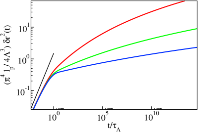
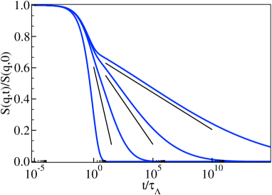
Figure 1: Time dependence of the transverse dynamic mean-square displacement $\delta r_{\perp L}^{2}(t)$ (MSD) and the dynamic structure factor $S(q,t)$. Left: The normalised MSD of a GWLC as a function of time $t$ for stretching parameters ${\cal E}=5$, 15, 35 (from top to bottom) for $f=0$. The straight line indicates the limiting power-law growth $\delta r_{\perp L}^{2}(t)\propto t^{3/4}$ of the MSD of an infinite weakly bending WLC. Right: The dynamic structure factor of a GWLC, evaluated numerically for $q^{2}=\ell_{p}\pi^{4}/\Lambda^{3}$ and stretching parameters ${\cal E}=0,5,15,35$ (from left to right). The straight lines indicate the logarithmic intermediate asymptotics calculated in equation (13).

4 Prestress

Before we come to the evaluation of further observables, we first want to consider the effect of tension on a GWLC. An (optional) constant tension $f$ was already included in our brief account of the ordinary WLC in section 2. However, we should certainly also expect an effect of any kind of external or internal stress onto the escape of the polymer over the free energy barriers represented by ${\cal E}$. Intuitively, the force is expected to “help the polymer over the free energy barriers”, but we cannot, of course, exclude the opposite effect, namely that the traps become under certain circumstances deeper upon applying a force. In any case, the natural way to introduce a force into this picture is via a tilting of the free energy landscape in the spirit of a Kramers escape rate model, i.e.

$${\cal E}\to{\cal E}\pm f/f_{T}\;,\qquad f_{T}\equiv k_{B}T/\Delta\;.$$ (10)

The minus sign corresponds to the force lowering the barrier. The length $\Delta$ should be interpreted as a characteristic width of the free energy wells and barriers. Accordingly, $f_{T}$ represents the scale of thermally induced force fluctuations, which are even present in absence of an applied stress.

The introduction of an external force in equation (10) may be seen as a simple heuristic method to address the rheology of prestressed networks or even of the nonlinear rheology of cytoskeletal networks. This is of considerable interest for potential applications of our model, since prestress is thought to be the crucial element needed for mimicking typical cell rheological behaviour using much simpler reconstituted networks [25, 26, 27, 28, 18]. There is, however, a subtle point involved in the interpretation of the force $f$ as arising from a prestress. For simplicity, we have tacitly assumed above that the force that pulls the test chain over the free energy barriers is identical to its backbone tension. This should not a priori be a problematic assumption for qualitative purposes. But a test polymer embedded into a cytoskeletal network or sticky biopolymer solution that was initially unstressed will generally have a conformation different from the stretched conformation of our free test chain equilibrated under the backbone tension $f$. As noted above, we do not attempt to address this problem, at the present stage. Altogether, after disregarding such potential modifications of the equilibrium conformation of the test chain by its surroundings and identifying the barrier lowering force with the backbone tension, $f$ remains to be related to the macroscopic shear stress. Consistent with our discussion of the shear modulus in section 7, below, we follow Ref. [29] in writing $\sigma=f/5\xi^{2}$, where $\xi\equiv(3/c_{p}L)^{1/2}$ is the mesh size of a semidilute solution of semiflexible polymers. Its relation to the polymer concentration $c_{p}$ and the numerical prefactors are of geometric origin. As a reminder of the tentative nature of the identification of $\sigma$ as an actual prestress we call $\sigma$ the “nominal prestress”.

5 Dynamic structure factor

For sufficiently long times $t\gg\zeta_{\perp}/\kappa q^{4}$, the dynamic structure factor $S(q,t)$ at scattering vector $q\gg\Lambda^{-1}$ follows from the transverse mean square displacement according to [30],

$$S(q,t)/S(q,0)\sim\exp\left[-q^{2}\delta r_{\perp L}^{2}(t)/4\right]\;.$$ (11)

The time dependence of the structure factor is plotted in figure 1. A pronounced logarithmic intermediate asymptotics is seen to develop for large ${\cal E}$. It can be calculated approximately as follows. First, we identify a logarithmic intermediate asymptotics in the MSD. At intermediate times the MSD takes the form

$$\delta r_{\perp L}^{2}(t)\sim\delta r_{\perp\Lambda}^{2}(\infty)+\frac{4\Lambda^{3}}{{\cal E}\ell_{p}\pi^{4}}\left[\gamma_{E}+\log(t/\tau_{\Lambda})\right]\qquad(1\ll t/\tau_{\Lambda}\ll{\cal E})\;,$$ (12)

for an unstressed chain ($f=0$). Here $\delta r_{\perp\Lambda}^{2}(\infty)$ contains the saturated contributions from the free WLC modes up to wavelength $\Lambda$. The GWLC part of the mode spectrum is asymptotically approximated by the logarithmic term. Expanding the exponential in equation (11) to leading order in the logarithmic contribution gives

$$\frac{S(q,t)}{S(q,0)}\sim\left[1-\frac{q^{2}\Lambda^{3}}{{\cal E}\ell_{p}\pi^{4}}\left(\gamma_{E}+\log\frac{t}{\tau_{\Lambda}}\right)\right]\exp\left[-\frac{q^{2}\delta r_{\perp\Lambda}^{2}(\infty)}{4}\right]$$ (13)

for the unstressed test chain. As demonstrated in figure 1, the numerically evaluated dynamic structure factor agrees with this approximation well beyond the time domain where the logarithmic contribution in the exponent of equation (11) is small. From the slope of the logarithmic tails of the structure factor in a semi-logarithmic plot the stretching parameter ${\cal E}$ is thus immediately inferred.

6 Microrheology

From the transverse MSD of a point on the polymer contour, we deduce the linear susceptibility $\alpha_{f}(\omega)$ (the subscript $f$ refers to the prestressing tension) to a transverse oscillating point force at frequency $\omega$ from the fluctuation dissipation theorem. It relates the imaginary part $\alpha_{f}^{\prime\prime}(\omega)$ of the susceptibility to the Fourier transform $\delta r_{\perp L}^{2}(\omega)$ of the MSD via $\alpha_{f}^{\prime\prime}(\omega)=-\omega\delta r_{\perp L}^{2}(\omega)/2k_{B}T$. The real part of $\alpha_{f}$ is then uniquely determined by the Kramers–Kronig relations, so that we find altogether

$$\alpha_{f}(\omega)=\frac{L^{3}}{k_{B}T\ell_{p}\pi^{4}}\sum_{n=1}^{\infty}\frac{1}{(n^{4}+n^{2}f/f_{L})(1+i\omega\tilde{\tau}_{n})}\;.$$ (14)

For better comparison with the macrorheological complex shear modulus, it is customary to report the inverse (up to a constant scale factor) $g^{*}_{f}(\omega)\propto 1/\alpha_{f}(\omega)$ of the susceptibility, which is called the “microrheological modulus”. Its real and imaginary parts $g_{f}^{\prime}(\omega)$ and $g_{f}^{\prime\prime}(\omega)$ are plotted in figure 2. The prestressing force $f$ is seen to compete with the stretching parameter ${\cal E}$ in raising/lowering the apparent power-law exponent of the low-frequency modulus. Its full effect is somewhat richer, because $f$ also affects the WLC mode amplitudes and relaxation times according to the explicit expressions provided in section 2.

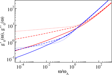
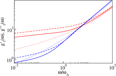
Figure 2: Frequency dependence of the real and imaginary parts $g_{f}^{\prime}(\omega)$, $g_{f}^{\prime\prime}(\omega)$ (red/blue curve) of the microrheological modulus, which is a common representation of the dynamic linear response to a transverse point force applied to a test polymer. The abscissa is normalised to $g_{f=0}^{\prime}(\omega_{\Lambda})$ (${\cal E}=0$). Left: ${\cal E}=$ 3 (solid), 10 (dashed), 35 (dotted) at vanishing prestress, $f=0$. Right: $f/f_{\Lambda}=$ 0 (solid), 1 (dashed), 2.4 (dotted) at fixed ${\cal E}=25$ with $f_{T}=0.1f_{\Lambda}$, $f_{\Lambda}$ being the Euler force for the interaction wavelength $\Lambda$.

7 The shear modulus

The microrheological modulus discussed in the preceding section should not be confused with the shear modulus measured by a macroscopic rheometer. While, in practice, the two quantities are sometimes hard to distinguish, this must be attributed to non-ideal (i.e. not point-like) probes such as colloidal beads used to transmit the force to the medium and to detect its deformation, which require additional considerations [31, 32]. Noninvasive techniques, such as quasi-elastic light scattering are more sensitive to the difference between the two response functions [19]. In the following, we present results based on the assumption that the macroscopic shear modulus is obtained by applying our GWLC prescription, equation (8), to the high frequency limiting form of the shear modulus [29]. The latter is a single polymer quantity due to the independent relaxation of the short wavelength modes that dominate the high frequency response. The results thus obtained for the frequency dependence of the real and imaginary parts $G_{\sigma}^{\prime}(\omega)$ and $G_{\sigma}^{\prime\prime}(\omega)$ of the shear modulus $G^{*}_{\sigma}(\omega)$ are displayed for various nominal prestresses $\sigma=f/5\xi^{2}$ in figure 3. In contrast to the microrheological modulus, the shear modulus is seen to develop a plateau that is sensitive to the prestress as a consequence of the underlying assumption [29] that the single polymers are stretched affinely upon applying a macroscopic shear stress. This assumption is presently under scrutiny [33, 34, 35], and might in the future have to be relaxed for modes of wavelength $\lambda_{n}\gtrsim\Lambda$.

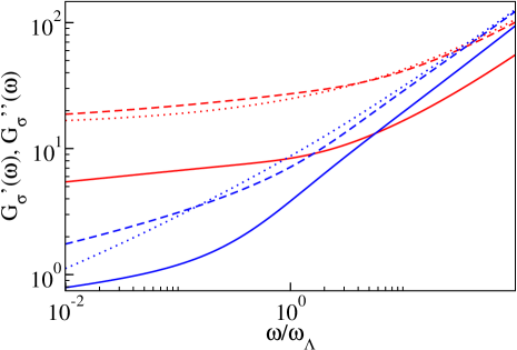
Figure 3: Frequency dependence of the real and imaginary parts $G_{\sigma}^{\prime}(\omega)$, $G_{\sigma}^{\prime\prime}(\omega)$ (red/blue curve) of the macroscopic shear modulus obtained by applying the GWLC prescription to the theoretical expression for the high-frequency limiting form of the shear modulus from Ref. [29] for various nominal prestresses $\sigma=f/5\xi^{2}$ corresponding to $f/f_{\Lambda}=$ 0 (solid), 2 (dashed), 2.45 (dotted) at ${\cal E}=25$, $f_{T}=0.1f_{\Lambda}$. The modulus has been normalised to $G_{\sigma=0}^{\prime}(\omega_{\Lambda})$ (${\cal E}=0$).

On the level of our simplifying assumptions, the shear modulus in the presence of a prestress is equivalent to the nonlinear differential shear modulus $K$ [5, 36]. It is therefore of some interest to evaluate the dependence of $|G^{*}|$ at a fixed frequency $\omega$ as a function of the nominal prestress $\sigma$, which then amounts to a characterisation of the nonlinear finite-time elasticity of the system. Via the force dependence of the bare WLC expressions of section 2, the prestress causes stress stiffening, i.e., a monotonic increase of $|G^{*}|$ with $\sigma$. In contrast, the exponential speed-up of the relaxation caused by the barrier-lowering effect of the generated tension according to equation (10) eventually overcompensates this stiffening for large stresses. This is analysed in figure 4 (left) for various stretching parameters. The limiting functional relation $|G_{\sigma}^{*}|\propto\sigma^{3/2}$ for the stiffening, which is only slowly approached for ${\cal E}\to\infty$ is an immediate consequence of the underlying affine assumption [29]. While there is some recent experimental support that this limiting behaviour is indeed measurable in actin bundle networks heavily crosslinked by scruin [36] (plausibly corresponding to ${\cal E}\to\infty$), experiments for actin/$\alpha-$actinin solutions [37], actin solutions homogeneously crosslinked by heavy meromyosion (HMM) in the rigor state [8], and pure actin solutions [19] rather reveal a continuity of stiffening relations. They suggest that the stiffening is much less universal than previously thought [6] and might depend on the degree of “glassiness” of the system, consistent with a finite stretching parameter ${\cal E}$ dependent on various control parameters such as crosslinker concentration, temperature and ionic strength. To some extent, observations of a weaker stiffening might also indicate a contribution of (non-affine) transverse modes, as these exhibit weaker stiffening; see the corresponding curves for the transverse microrheological response in figure 4 (right), which converge to the asymptotic stiffening relation $|g_{f}^{*}|\propto f$ for very large ${\cal E}$. But the GWLC does neither require nor support a strict correspondence of network affinity to the nonlinear response as recently postulated [5].

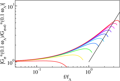
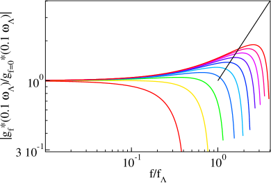
Figure 4: The normalised moduli as a function of prestress. Left: The shear modulus $|G_{\sigma}^{*}|/|G_{\sigma=0}^{*}|$, which is, under the assumptions stated in the main text, equivalent to the nonlinear differential shear modulus, evaluated at a fixed frequency $\omega=0.1\omega_{\Lambda}$ as a function of the normalised tension $f/f_{\Lambda}$ corresponding to a nominal prestress $\sigma=f/5\xi^{2}$ for various ${\cal E}=4\dots 40$ (from bottom to top) at $f_{T}=0.1f_{\Lambda}$. The straight line indicates the asymptotic stiffening power-law to which the stiffening curves slowly converge in the limit ${\cal E}\to\infty$. Right: The corresponding curves for transverse the microrheological modulus.

8 Cytoskeletal networks and rough free energy landscapes

While free energy landscapes certainly represent an appealing intuitive framework for the discussion of many properties of complex disordered media, it is notoriously hard to calculate their pertinent features from first principles [38]. In the remainder, we want to give some qualitative arguments as to why we expect the rough free energy landscapes alluded to in our motivation of the GWLC to be characteristic of cytoskeletal networks in vitro and in vivo. We distinguish two contributions to the free energy: direct contributions from a bare polymer-polymer pair interaction potential, and collective cageing or entanglement effects. For the typical biopolymer solutions and networks found in cells and tissues both cannot easily be derived microscopically or reduced to known elementary atomic pair interactions: the former because of the strongly collective, heterogeneous, anisotropic etc. nature of protein interactions [39], the latter because semidilute polymer solutions represent a highly correlated state of matter [40].

Figure 5: Schematic sketch of a hypothetical bare pair potential $U(r)$ suggested to provide an approximate representation of the complex interactions between cytoskeletal constituents.

While protein interactions remain poorly understood, many observations hint at (unspecific, e.g. hydrophobic) adhesive contact interactions incompletely screened by electrostatic repulsion [41]. It is thus not implausible that direct interactions of cytoskeletal elements can approximately be represented by a pair potential $U(r)$ of the qualitative form sketched in figure 5 [42], which features a narrow energy barrier. Such “enthalpic” barriers slow down the mode relaxation by an Arrhenius factor, which scales exponentially in the barrier height. The barriers would thus yield substantial contributions to ${\cal E}$ without seriously affecting the thermodynamics of the system. The less obvious free energy contributions from cageing and entanglement are typically postulated in generic free-volume theories [43], as their calculation from first principles remains one of the major challenges in the theory of structural glasses [44]. For semiflexible polymer networks they can be estimated within the tube model [45], which suggests a contribution ${\cal E}\simeq 1$. Accordingly, a plausible estimate for the effective well width $\Delta$ should be given by the tube diameter, which scales like $\xi^{6/5}\ell_{p}^{-1/5}$ [24] in a semidilute semiflexible polymer solution and is estimated to assume values in the range of some 10 to 100 nm for typical in vitro polymerised actin solutions. In any case, simple exponential scaling of the relaxation times in ${\cal E}$ and in the wavelength $\lambda$, as postulated in equation (8) seems plausible for an entangled solution of weakly bending sticky polymers.

It is important to realise that the parameters ${\cal E}$ and $\Delta$ are to be understood as effective parameters. They cannot generally be expected to correspond directly to some salient features of a bare interaction potential as sketched in figure 5 nor to the experimentally more accessible coarse-grained interactions between adjacent polymer segments of length $\Lambda$. (The latter can be roughly thought of as a smeared-out version of the former, due to the effect of thermal undulations of the polymers and possible compliant crosslinkers [46].)

The above suggestion to interpret ${\cal E}$ essentially as a kind of kinetic “stickiness” parameter for cytoskeletal polymers might have interesting implications as to the physiological role played by the broad class of actin binding proteins such as crosslinkers and molecular motors. While little is known about the microscopic interactions between cytoskeletal polymers, even less is known about how they might be affected by these proteins. Yet it seems plausible that the predominant effect of most crosslinkers can be subsumed into the parameter ${\cal E}$. Also, while current approaches to the active rheology of cells [10, 11, 47] put much emphasis on the dynamic role of molecular motors in causing transport and motion, some of them might well play a less flamboyant role most of the time: namely adjusting the effective stickiness ${\cal E}$ and tension $\sigma$ to tune the viscoelastic properties of the cytoskeleton while saving it from glassy arrest [48].

9 Conclusion

In summary, we have presented a simple modification of the standard model of a semiflexible polymer (the WLC), which we call the glassy wormlike chain (GWLC), and which is obtained by an exponential stretching of the relaxation spectrum of the WLC. The striking resemblance of the predicted mechanical observables with rheological data for cells and reconstituted cytoskeletal model systems naturally suggests that these systems must exhibit strong rheological redundancy. In fact, the perplexing universality and robustness of the mechanical performance of biological cells and tissues against structural modifications by drugs and mutations has been an enigma in cell biology for quite some time [49, 13]. Our glassy wormlike chain model offers a very economical explanation in terms of the difference between the stretching parameter ${\cal E}$ and the prestress $\sigma$ (in natural units). If changes in the structure and interactions of the cytoskeleton affect its rheological properties chiefly via ${\cal E}$ and $\sigma$, the potential for mutual compensation appears indeed enormous. This leads us to the suggestion that a microscopic calculation of the various anticipated contributions to ${\cal E}$ will be one of the major challenges for future theoretical work aiming to explain the rheology of cells and in vitro reconstituted models of the cytoskeleton.

References

References

- [1] A. R. Bausch and K. Kroy, Nature Physics 2, 231 (2006).
- [2] F. Wottawah et al., Physical Review Letters 94, 098103 (2005).
- [3] P. Fernandez, P. A. Pullarkat, and A. Ott, Biophys. J. 90, 3796 (2006).
- [4] D. C. Morse, Phys. Rev. E 63, 031502 (2001).
- [5] M. L. Gardel et al., Science 304, 1301 (2004).
- [6] C. Storm et al., Nature 435, 191 (2005).
- [7] J. Liu et al., Phys. Rev. Lett. 96, 118104 (2006).
- [8] R. Tharmann, M. M. A. E. Claessens, and A. R. Bausch, Phys. Rev. Lett. 98, 088103 (2007).
- [9] J. Guck et al., Biophys. J. 88, 3689 (2005).
- [10] Y. Hatwalne, S. Ramaswamy, M. Rao, and R. A. Simha, Phys. Rev. Lett. 92, 118101 (2004).
- [11] K. Kruse et al., Phys. Rev. Lett. 92, 078101 (2004), ibid. 93 (2004) 099902(E).
- [12] D. Mizuno, C. Tardin, C. F. Schmidt, and F. C. MacKintosh, Science 315, 370 (2007).
- [13] B. Fabry et al., Phys. Rev. Lett. 87, 148102 (2001).
- [14] P. Sollich, F. Lequeux, P. Hébraud, and M. E. Cates, Phys. Rev. Lett. 78, 2020 (1997).
- [15] L. Cipelletti and L. Ramos, J. Phys.: Condens. Matter 17, R253 R285 (2005).
- [16] L. Deng et al., Nature Materials 5, 636 (2006).
- [17] B. Hoffman, G. Massiera, K. Citters Van, and J. Crocker, Proc. Natl. Acad. Sci. U.S.A. 103, 10259 (2006).
- [18] N. Rosenblatt et al., Phys. Rev. Lett. 97, 168101 (2006).
- [19] C. Semmrich et al., unpublished.
- [20] R. Ananthakrishnan et al., Curr. Sci. 88, 1434 (2005).
- [21] O. Hallatschek, E. Frey, and K. Kroy, Phys. Rev. E 75, 031905 (2007).
- [22] J. J. Brey and A. Prados, Phys. Rev. E 63, 021108 (2001).
- [23] C. Monthus and J. P. Bouchaud, J. Phys. A: Math. Gen 29, 3847 (1996).
- [24] A. N. Semenov, J. Chem. Soc. Faraday Trans. 86, 317 (1986).
- [25] N. Wang et al., Am. J. Physiol. Cell Physiol. 282, C606 (2002).
- [26] D. E. Ingber, J. Cell. Sci. 116, 1157 (2003).
- [27] A. W. C. Lau et al., Phys. Rev. Lett. 91, 198101 (2003).
- [28] M. L. Gardel et al., Proc. Natl. Acad. Sci. U.S.A. 103, 1762 (2006).
- [29] F. Gittes and F. C. MacKintosh, Phys. Rev. E 58, R1241 (1998).
- [30] K. Kroy and E. Frey, in Scattering in Polymeric and Colloidal Systems, edited by W. Brown and K. Mortensen (Gordon and Breach, ADDRESS, 2000), Chap. 5, pp. 197–248.
- [31] D. Chen et al., Phys. Rev. Lett. 90, 108301 (2003).
- [32] T. M. Squires and J. F. Brady, Phys. Fluids 17, 073101 (2005).
- [33] D. A. Head, A. J. Levine, and F. C. MacKintosh, Phys. Rev. Lett. 91, 108102 (2003).
- [34] B. A. DiDonna and T. C. Lubensky, Phys. Rev. E 72, 066619 (2005).
- [35] C. Heussinger and E. Frey, Phys. Rev. Lett. 97, 105501 (2006).
- [36] M. L. Gardel et al., Phys. Rev. Lett. 93, 188102 (2004).
- [37] J. Y. Xu, Y. Tseng, and D. Wirtz, J. Biol. Chem. 275, 35886 (2000).
- [38] D. J. Wales, Energy Landscapes (Cambridge University Press, Cambridge, 2003).
- [39] R. P. Sear, Curr. Op. Coll. Int. Sci. 11, 35 (2005).
- [40] L. Schäfer, Excluded Volume Effects in Polymer Solutions as Explained by the Renormalization Group (Springer, Berlin, 1999).
- [41] R. Piazza, J. Colloid and Interface Sci. 8, 515 (2004).
- [42] M. Hosek and J. X. Tang, Phys. Rev. E 69, 051907 (2004).
- [43] R. Stinchcombe and M. Depken, Phys. Rev. Lett. 88, 125701 (2002).
- [44] P. D. Gujrati, S. S. Rane, and A. Corsi, Phys. Rev. E 67, 052501 (2003).
- [45] K. Kroy, Curr. Opin. Colloid Interface Sci. 11, 55 (2006).
- [46] B. Wagner et al., Proc. Natl. Acad. Sci. USA 103, 13974 (2006).
- [47] T. Shen and P. G. Wolynes, Phys. Rev. E 72, 041927 (2005).
- [48] B. Humphrey et al., Nature 416, 413 (2002).
- [49] E. Sackmann, in Modern Optics, Electronics, and High Precision Techniques in Cell Biology, edited by G. Isenberg (Springer, Heidelberg, 1997), Chap. 11, pp. 213–259.