Going beyond perturbation theory: Parametric Perturbation Theory

Abstract

We devise a non–perturbative method, called Parametric Perturbation Theory (PPT), which is alternative to the ordinary perturbation theory. The method relies on a principle of simplicity for the observable solutions, which are constrained to be linear in a certain (unphysical) parameter. The perturbative expansion is carried out in this parameter and not in the physical coupling (as in ordinary perturbation theory). We provide a number of nontrivial examples, where our method is capable to resum the divergent perturbative series, extract the leading asymptotic (strong coupling) behavior and predict with high accuracy the coefficients of the perturbative series. In the case of a zero dimensional field theory we prove that PPT can be used to provide the imaginary part of the solution, when the problem is analytically continued to negative couplings. In the case of a $\phi^{4}$ lattice model $1+1$ and of elastic theory we have shown that the observables resummed with PPT display a branch point at a finite value of the coupling, signaling the transition from a stable to a metastable state. We have also applied the method to the prediction of the virial coefficients for a hard sphere gas in two and three dimensions; in this example we have also found that the solution resummed with PPT has a singularity at finite density. Predictions for the unknown virial coefficients are made.

I Introduction

For the majority of the problems in Physics no exact analytical solution is known and it is a common procedure to resort to Perturbation Theory (PT) PT1 ; PT2 ; PT3 ; PT4 . The fundamental idea behind perturbation theory is that, if a given problem is solvable for a particular value of a parameter, then one can obtain analytical approximations to the solution in a close neighborhood of this value, by Taylor expanding in that parameter. Calling $g$ this parameter and $g_{0}$ the value for which an exact analytical solution is known, then the results obtained with perturbation theory will be, to a given order, polynomials in $(g-g_{0})$. The perturbative series obtained by considering all the terms of the expansion will in general have a finite radius of convergence, $r$, which in some cases could even be zero and therefore the series would be divergent for all $g\neq 0$. Actually divergent series are usually expected from the application of PT to quantum field theory, as first observed by Dyson in the case of Quantum Electrodynamics (QED)Dyson52 . Another well–known example of divergent series is given by the quantum anharmonic oscillator, whose perturbative coefficients for the energy of the ground state have been calculated by Bender and Wu in Bender and proved to have a factorial growth.

Although the pertubative series provide in many cases the only systematic approach to the solution of a problem, they are not always useful, since they are confined to a restricted region for the physical parameters, $|g-g_{0}|<r$. Outside this region, the physics becomes nonperturbative and cannot be described directly in terms of the original series. For quite a long time physicists have been interested into finding a bridge from the perturbative to the non–perturbative region. Several methods have been developed which allow to extract the non–perturbative behavior from the perturbative series: among such methods we would like to mention the Borel and Padé approximantsBenderOrzag ; PT1 and nonlinear transformations Weniger89 .

Methods which are alternative to PT should retain on one hand the ability to provide a sistematic analytical approximation to a given problem, and on the other hand they should remain valid even in the nonperturbative region, never leading to divergent series. Over the years new ideas have allowed to devise methods which comply with these requirements. The Linear Delta Expansion (LDE) lde and the Variational Perturbation Theory (VPT) Klei04 are two examples of non–perturbative methods. Roughly speaking these methods work by introducing in a problem an artificial parameter and turn the original problem into a new one with a modified perturbation. The optimization of the “perturbative” results to a given order with respect to the artificial parameter is usually obtained through the Principle of Minimal Sensitivity (PMS)Ste81 and leads to expressions which are non–polynomials in the physical parameters and therefore non–perturbative.

In this paper we will explore a new a path, which is also described in shorter letter: the method that we have devised, which we have called Parametric Perturbation Theory (PPT) method, is based on few simple ideas. The first one, which we will refer to as Principle of Absolute Simplicity (PAS), is that we do not want to calculate the observable (energy, frequency, etc.) directly as a polynomial in the physical coupling $g$, as done in PT, but that this observable should have the simplest possible form (linear) in a given unphysical parameter $\varrho$; the second idea is that the perturbation theory must be carried out in $\varrho$ and that the functional relation $g=g(\varrho)$ must comply with the Principle of Absolute Simplicity to the order to which the calculation is done. This will allow to determine the relation between $g$ and $\rho$ and in turn to obtain the observable as a parametric function of $\varrho$.

The paper is organized as follows: in Section II we develop the Parametric Perturbation Theory for a problem of nonlinear oscillations in classical mechanics and show that at finite order it provides extremely accurate approximations for the frequencies and for the solutions of the problem; in Section III we show that the PPT approach can be applied directly on the perturbative series and discuss the performance of our method in the case of non trivial examples, with divergent perturbative series. Finally, in Section IV we draw our conclusions.

II The method

Consider a model which depends on a parameter $g$, and which is solvable when $g=0$. The application of PT to this problem to a finite order yields a polynomial in $g$. Calling $r$ the radius of convergence of the perturbative series, the direct use of PT must be restricted to $|g|<r$, as previously discussed. However, the misbehavior of the perturbative series for a physical observable $\mathcal{O}$ is the result of having expanded in a parameter, $g$, which is not optimal. If one knew the exact solution to the problem, i.e. $\mathcal{O}=f(g)$, then this solution could be considered as a polynomial of order one in the variable $\varrho=f(g)$. Although this observation by itself cannot be used as a constructive principle, we may adopt the philosophy that the perturbative series for the observable can be simpler and convergent in all the domain, if it is cast in terms of a suitable parameter $\varrho$.

Only if such parameter, by luck or ability, turns out to be the $\varrho=f(g)$ discussed above, the exact solution is obtained. The goal, therefore, is to progressively build this parameter $\varrho$ to yield an expression for $\mathcal{O}$ as simple as possible. In this framework the perturbative expansion is carried out in $\varrho$ and all the physical quantities in the problem are expressed as functions of $\varrho$. In particular we have now that $g=g(\varrho)$. While the ordinary perturbation theory works by calculating the contributions to higher orders in $g$, each term of higher order refining the result to lower order, the approach approach is the opposite: we carry out a perturbative calculation in $\varrho$, and then determine order by order the form of $g=g(\varrho)$ so that the observable $\mathcal{O}(\varrho)$ can be a order one polynomial in $\varrho$. This is in essence the Principle of Absolute Simplicity.

Having given the general ideas of the method we proceed to examine its implementation in a concrete problem. We consider the classical nonlinear oscillations of a point mass described by the equation (Duffing equation)

$$\frac{d^{2}x}{dt^{2}}+x(t)=-gx^{3}(t)\ .$$ (1)

The Lindstedt-Poincaré method can be used to obtain a perturbative expansion of the squared frequency $\Omega^{2}$ of the oscillations in powers of $g$ PT1 ; PT3 ; PT4 . The method works by defining an absolute time scale, independent of $g$ and by then fixing the coefficients of the expansion of $\Omega^{2}$ so that the secular terms in the expansion are eliminated at each order. Working through order $(gA^{2})^{5}$ one finds

$$\Omega^{2}\approx 1+\frac{3gA^{2}}{4}-\frac{3g^{2}A^{4}}{128}+\frac{9g^{3}A^{6}}{512}-\frac{1779g^{4}A^{8}}{131072}+O\left[(gA^{2})^{5}\right]\ ,$$ (2)

$A$ being the amplitude of oscillations.

We now proceed to implement our method. The first step is to define a functional relation between $g$ and the perturbative parameter of the expansion, $\varrho$. For example, we choose

$$g(\varrho)=\varrho\ \frac{1+\sum_{n=1}^{\bar{N}}c_{n}\varrho^{n}}{1+\sum_{n=1}^{\bar{N}}d_{n}\varrho^{n}}\ ,$$ (3)

where the coefficients $c_{n}$ and $d_{n}$ are unknown constants to be later determined. The parameter $\bar{N}$ is related to the order to which the calculation is performed, since the number of coefficients $c_{i}$ and $d_{i}$ needs to match the number of conditions available at a given order.

The reader may wonder the reason of the particular choice made in eq. (3): the functional relation between $g$ and $\varrho$ can be more general than eq. (3), although it is not completely arbitrary since it must reproduce all the terms in the perturbative expansion when the relation between $g$ and $\varrho$ is inverted. The choice made here takes into account this fact and also the leading asymptotic behavior of the frequency, $\lim_{g\rightarrow\infty}\Omega^{2}\propto g$.

We now follow the standard procedure of the LP method and introduce an absolute time $\tau\equiv\Omega(\varrho)\ t$. Applying the PAS we choose this relation to be

$$\Omega^{2}(\rho)=\alpha_{1}+\alpha_{2}\varrho\ ,$$ (4)

where $\alpha_{1,2}$ are coefficients to be determined. We also expand the solution as

$$y(\tau)=\sum_{n=0}^{\infty}y_{n}(\tau)\ \left(\frac{g}{\varrho}-1\right)^{n}\ .$$ (5)

The reader familiar with the LP method will recognize the profoundly different character of the present approach: in the LP method the observable, i.e. $\Omega^{2}$, is expressed as a series in powers of $g$, whose coefficients are determined by the condition that secular terms are eliminated at each order; here we impose that $\Omega^{2}$ has the simplest possible form when expressed in terms of $\varrho$, and we let $g(\varrho)$ to contain arbitrary powers of $\varrho$. In detail, we transform the original equation into the new equation

$$\Omega^{2}(\varrho)\ \frac{d^{2}y}{d\tau^{2}}+y(\tau)=-g(\varrho)\ y^{3}(\tau)\ .$$ (6)

For sake of simplicity we will limit ourselves to work through order $\varrho^{3}$ and solve the differential equations resulting at each order in $\varrho$. The elimination of the secular term to order one yields $\alpha_{1}=3A^{2}/4$, as in standard LP method ($\alpha_{0}=1$). The solutions to order $0$ and $1$ are $y_{0}(\tau)=A\cos\tau$ and $y_{1}(\tau)=\frac{A^{3}}{32(c_{1}-d_{1})}\ (-\cos\tau+\cos 3\tau)$.

The elimination of the secular term to second order provides the condition

$$d_{1}=c_{1}-\frac{A^{2}}{32}$$ (7)

and the solution

$$y_{2}(\tau)=\left(23A-\frac{32c_{1}}{A}\right)\cos\tau-\left(24A-\frac{32c_{1}}{A}\right)\cos 3\tau\ .$$ (8)

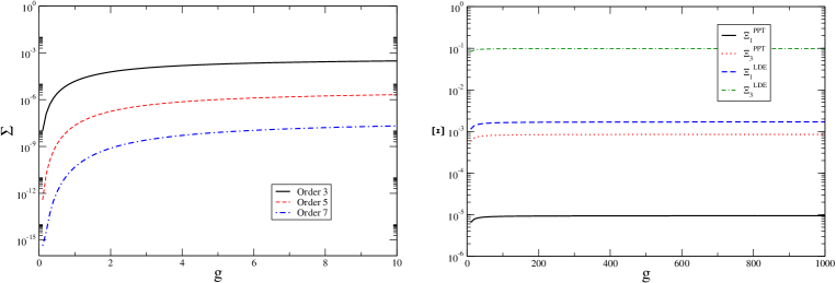
Figure 1: (color online) Left panel: Error over the square frequency, $\Sigma=1-\Omega^{2}_{approx}/\Omega^{2}_{exact}$, calculated to order 3,5 and 7 (solid, dashed and dot-dashed curves); Right panel: Error over the first two Fourier coefficients calculated to order 3 using PPT and the LDE approach of Amore07 .

Finally, one can determine $c_{1}$ to cancel the secular term to third order, $c_{1}=\frac{23}{32}A^{2}$, and correspondingly $d_{1}=\frac{11}{16}A^{2}$. The solution to third order thus reads

$$y_{3}(\tau)=5A\cos\tau-4A\cos 3\tau-2A\cos 5\tau+A\cos 7\tau\ .$$ (9)

To order $\varrho^{3}$ we therefore find

$$g \approx \varrho\ \frac{32+23\varrho A^{2}}{32+22\varrho A^{2}}\ ,$$ (10)

which can be inverted and used to express the frequency directly in terms of $g$:

$$\Omega^{2} \approx 1+\frac{3}{4}\varrho A^{2}=\frac{11}{23}+\frac{33}{92}gA^{2}+\frac{3}{92}\sqrt{\left(121gA^{2}+384\right)gA^{2}+256}\ .$$ (11)

Notice that this expression is non–perturbative in $gA^{2}$ and that it provides a maximum error $\Sigma=\lim_{gA^{2}\rightarrow\infty}\left(1-\Omega^{2}/\Omega^{2}_{exact}\right)\approx 5.27\times 10^{-4}$. This error is much smaller that then the one obtained to third order in Amore03 using the Linear Delta Expansion, i.e. $\Omega^{2}_{LDE}=\frac{69gA^{4}+192gA^{2}+128}{96gA^{2}+128}$ ( in which case one has $\Sigma_{LDE}=\lim_{gA^{2}\rightarrow\infty}\left(1-\Omega^{2}_{LDE}/\Omega^{2}_{exact}\right)\approx 1.36\times 10^{-2}$).

At the same time PPT provides highly accurate estimates for the Fourier coefficients of the solution, $c_{n}$. In the right panel of fig.1 we have plotted the error defined as $\Xi_{n}\equiv\left|c_{n}^{approx}/c_{n}^{exact}-1\right|$ as function of $g$ and compared our results with the already excellent results of Amore07 .

At this point the reader should recognize that, if one is interested only in frequency and not in the solution, it is possible to determine the coefficients $c_{n}$ and $d_{n}$ to a given order with a minimal effort directly from the coefficients of the perturbative series. The procedure consists of first substituting $g=g(\varrho)$ inside the perturbative series, and then expanding around $\varrho=0$: the unknown coefficients $c_{n}$ and $d_{n}$ are then used to suppress the nonlinear behavior in $\varrho$ inside $\Omega^{2}$. Following this simple procedure we have produced the result to order $5$ and $7$ in the left panel of Fig.1.

III Resummation of perturbative series

In many cases the perturbative results for a given problem are known only to a finite order since the calculation of each higher order involves increasing technical difficulties. For example, the calculation of observables in Quantum Field Theory at a given order in PT requires to take into account a number of Feynman diagrams which rapidly grows with the order of the perturbation, the calculation of the higher order (multiloop) diagrams being more and more challenging.

For this reason it is desirable to have a procedure which, using only a finite number of perturbative coefficients, may extract the essential physical behavior of the solution and possibly predict a number of unknown perturbative coefficients. We will show now that this result can be efficiently achieved using our method.

III.1 Anharmonic oscillator

Consider the quantum anharmonic oscillator

$$\hat{H}=\frac{\hat{p}^{2}}{2}+\frac{x^{2}}{2}+gx^{4}\ .$$ (12)

The series obtained with perturbation theory for this problem is divergent and its coefficients behave as

$$b_{n}\approx(-1)^{n+1}\sqrt{6/\pi^{3}}\ \Gamma(n+1/2)3^{n}$$ (13)

for $n\rightarrow\infty$ as shown in  Bender . These coefficients can be also obtained exactly, using the recursion relations given by Bender and Wu in Bender . The resummation of this perturbative series has been considered by several authors, using different techniquesPT1 ; PT2 ; LMSW69 ; WCV93 ; Ivanov95 ; Weni96 ; CWBS96 ; SG98 ; Home ; Nuñez ; RB06 ; KJ95 .

We will follow the philosophy of our method and define a functional relation between the physical coupling $g$ and the unphysical parameter $\varrho$. In principle this relation can be expressed by mean of an arbitrary function, but it can also use information coming from the strong coupling regime, where the energy goes like $E_{0}\propto g^{1/3}$ as $g\rightarrow\infty$. For example we can choose

$$g(\varrho)=\varrho\ \left[\frac{1+\sum_{n=1}^{\bar{N}+1}c_{n}\varrho^{n}}{1+\sum_{n=1}^{\bar{N}}d_{n}\varrho^{n}}\right]^{2},$$ (14)

which has the correct asymptotic behavior for $g\rightarrow\infty$, provided that the denonimator does not vanish for $\varrho>0$. The unknown coefficients $c_{n}$ and $d_{n}$ in this expression will be determined so that the ground state energy is linear in the unphysical parameter, as required by the PAS, i.e.

$$E_{0}=b_{0}+b_{1}\varrho\ .$$ (15)

Choosing $\bar{N}=3$, corresponding to use only the first $6$ perturbative coefficients, we can fully determine the coefficients $c_{n}$ and $d_{n}$:

$$c_{1} = \frac{3111725471}{109345364}\ ,\ c_{2}=\frac{292194444505}{1749525824},c_{3}=\frac{1136953355311}{6998103296}$$

$$d_{1} = \frac{730092771}{27336341}\ ,\ d_{2}=\frac{215945995035}{1749525824}\ .$$

Working to this order it is possible to extract the leading coefficient of the strong coupling series

$$\alpha_{0} = \lim_{\varrho\rightarrow\infty}\frac{b_{0}+b_{1}\varrho}{g(\varrho)}=3\left(\frac{215945995035}{2273906710622}\right)^{2/3}\approx 0.624458\ ,$$ (16)

which should be compared with the fairly precise results of PT1 ; Fernandez97 ; KJ95 , $\alpha_{0}=0.66798625915577710827096$. In the opposite limit, $g\rightarrow 0$, the energy calculated with the PPT can be cast in terms of $g$ after inverting (14):

$$E_{0} \approx \frac{1}{2}+\frac{3g}{4}-\frac{21g^{2}}{8}+\frac{333g^{3}}{16}-\frac{30885g^{4}}{128}+\frac{916731g^{5}}{256}-\frac{65518401g^{6}}{1024}+\frac{9397438011180958461g^{7}}{7166057775104}$$ (17)

$$- \frac{5778726063447202343420510691g^{8}}{195893798965944254464}+\frac{120539916022637946813802592301161300277g^{9}}{171360630026191984864597639168}$$

$$- \frac{20343642843373228886854633070691634893375294933\ g^{10}}{1171093154092705757431369973022851072}+O\left[g^{11}\right]$$

which is correct up to order $g^{6}$. In Table 1 we compare the exact perturbative coefficients going from the order $g^{7}$ to order $g^{10}$ with the approximate ones predicted by the PPT using $\bar{N}=3$. The last column displays the error $\Sigma_{n}\equiv 100\times\left|b_{n}^{[3,2]}/b_{n}^{exact}-1\right|$.

Table 1: Comparison of the exact perturbative coefficients for the anharmonic oscillator with the approximate coefficients obtained with PPT using $\bar{N}=3$.

n	$b_{n}^{(exact)}$	$b_{n}^{[3,2]}$	error ($\%$)
7	$\frac{2723294673}{2048}$	$\frac{9397438011180958461}{7166057775104}$	$1.399$
8	$-\frac{1030495099053}{32768}$	$-\frac{5778726063447202343420510691}{195893798965944254464}$	$6.19$
9	$\frac{54626982511455}{65536}$	$\frac{120539916022637946813802592301161300277}{171360630026191984864597639168}$	$15.61$
10	$-\frac{6417007431590595}{262144}$	$-\frac{20343642843373228886854633070691634893375294933}{1171093154092705757431369973022851072}$	$29.03$

The reader could argue that the quality of the results that we have obtained is due to having taken into account the exact asymptotic behavior of $E_{0}$ for $g\rightarrow\infty$. We will now show that our method allows one to optimize the asymptotic behavior of the approximate solution, even in the case where the exact behavior is unknown. We consider the approximations corresponding to

$$g(\varrho)=\varrho\ \left[\frac{1+\sum_{n=1}^{\bar{N}_{u}}c_{n}\varrho^{n}}{1+\sum_{n=1}^{\bar{N}_{d}}d_{n}\varrho^{n}}\right]^{2},$$ (18)

fixing $\bar{N}_{u}+\bar{N}_{d}=5$ as in the previous case. We can compare the first coefficient predicted by our method, $b_{7}$, using the different sets. These coefficients are displayed in the first row of Table 2; the second row displays the error (in $\%$) with respect to the exact coefficient, shown in Table 1. The set $[3,2]$ previously considered provides the lowest error and therefore selects the correct asymptotic behavior.

This example shows that, even in the unfortunate case where the asymptotic behavior of the energy is unknown, it is possible to extract some information on the strong coupling regime directly from the perturbative series, using a limited number of perturbative coefficients.

Table 2: Comparison of the exact perturbative coefficients for the anharmonic oscillator with the approximate coefficients obtained with PPT using $\bar{N}=3$.

	$b_{7}^{[5,0]}$	$b_{7}^{[4,1]}$	$b_{7}^{[3,2]}$	$b_{7}^{[2,3]}$	$b_{7}^{[1,4]}$	$b_{7}^{[0,5]}$
$b_{7}$	$\frac{141732231981}{131072}$	$\frac{49825588453972797}{38645137408}$	$\frac{9397438011180958461}{7166057775104}$	$\frac{31966088112282317691}{24592236412928}$	$\frac{67034980866178137}{52602994688}$	$\frac{134498076375}{131072}$
error ($\%$)	$22.97$	$3.13$	$1.399$	$2.299$	$4.34$	$29.58$

In Fig.2 we have plotted the exact energy (numerical) as a function of $g$ (squares) and we have compared it with the results of PPT applied to $3$ different orders, all reproducing the exact asymptotic behavior. Our results approach the numerical result as $\bar{N}$ is increased.

III.2 A PT symmetric hamiltonian

The complex hamiltonian

$$\hat{H}=p^{2}+\frac{1}{4}x^{2}+igx^{3}\ ,$$ (19)

has been the first example of a PT symmetric hamiltonian which has a completely real spectrum to be discovered. Bender and Dunne have studied in Bender98 the large order perturbative expansion of the ground state energy of this hamiltonian finding that the coefficients of this series grow as

$$b_{n}\approx(-1)^{n+1}\frac{60^{n+1/2}}{(2\pi)^{3/2}}\ \Gamma(n+1/2)\left[1-O(1/n)\right].$$ (20)

Table I of Bender98 contains the first 20 coefficients of the perturbative series. In a recent paper Bender and Weniger BW01 have provided numerical evidence that the perturbative series for this PT symmetric hamiltonian is Stieltjes, using the first $193$ nonzero coefficients.

We will here use this model to obtain a further test of PPT. We assume the functional relation

$$g(\varrho)=\sqrt{\varrho\ \left[\frac{1+\sum_{n=1}^{\bar{N}}c_{n}\varrho^{n}}{1+\sum_{n=1}^{\bar{M}}d_{n}\varrho^{n}}\right]}\ ,$$ (21)

where the difference $\bar{N}-\bar{M}$ constrains the asymptotic behavior, which is not known exactly in this case. Notice that the square root in the definition of $g$ is a consequence of the fact that the perturbative series contains only even powers of $g$ Bender98 . In Fig.4 we have compared the exact numerical results of the last column of Table III of Bender98 with the calculation obtained with PPT using three different sets of $(\bar{N},\bar{M})$, which correspond to the same number of conditions . Our results suggest that the asymptotic behavior of the energy is approximately $E_{0}\propto\sqrt{g}$ for $g\rightarrow\infty$.

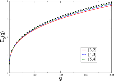
Figure 2: (color online) Ground state energy of the anharmonic oscillator as a function of $g$. The squares are numerical results, the curves correspond to the results obtained with PPT to different orders.

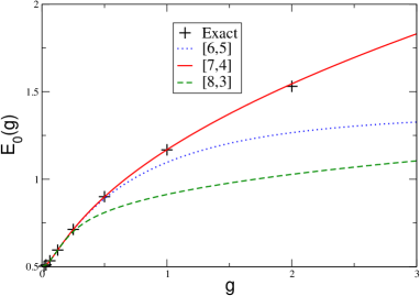
Figure 3: (color online) Ground state energy of the anharmonic oscillator as a function of $g$. The squares are numerical results, the curves correspond to the results obtained with PPT to different orders.

III.3 Zero dimensional $\phi^{4}$ theory

Integrals of the form

$$E(g)=\int_{0}^{+\infty}e^{-x^{2}-gx^{4}}dx$$ (22)

can be used as a model of a $\phi^{4}$ in zero dimensions JZJ ; BDJ93 ; BDJ94 . As for the case of higher dimensional field theories, the perturbative series for this model is divergent. The authors of BDJ93 ; BDJ94 have proved that the Linear Delta Expansion (LDE) is able to deal with this problem and that it provides results which rapidly converge to the exact value.

The integral in eq.(22) admits an exact analytical solution which is given by

$$E(g)=\frac{e^{\frac{1}{8g}}}{4\sqrt{g}}\ K_{1/4}\left(\frac{1}{8g}\right)\ ,$$ (23)

where $K_{1/4}(g)$ is the Bessel function of order $1/4$. Notice that for negative values of $g$ this expression acquires an imaginary part, signaling that the system becomes metastable.

We will now analyze this problem with the help of PPT. We choose the functional relation

$$g(\varrho)=\varrho\ \left[\frac{1+\sum_{n=1}^{\bar{N}}c_{n}\varrho^{n}}{1+\sum_{n=1}^{\bar{N}+1}d_{n}\varrho^{n}}\right]^{5},$$ (24)

which allows one to obtain the correct asymptotic behavior, $E(g)\propto g^{-1/4}$ as $g\rightarrow\infty$.

As usual the application of the PPT method requires that the coefficients $c_{n}$ and $d_{n}$ corresponding to a given $\bar{N}$ be determined by imposing the PAS, i.e. by asking that the observable $E(g)$ be linear in the parameter $\varrho$. Using three different sets, corresponding to $\bar{N}=1,2$ and $3$ we have observed that our results converge quickly to the exact analytical result (see the left panel in Fig.4).

We will however move further and concentrate over the best set, $\bar{N}=3$. In this case the relation between $g$ and $\varrho$ is given by

$$g(\varrho)\approx\frac{\rho\left(2924.98\varrho^{3}+881.78\varrho^{2}+58.83\varrho+1\right)^{5}}{\left(-1737.20\varrho^{4}+2243.93\varrho^{3}+832.17\varrho^{2}+57.96\varrho+1\right)^{5}}\ .$$ (25)

Since $\varrho_{0}=-0.0593$ is a zero of the denominator, $\lim_{\varrho\rightarrow\varrho_{0}}g(\varrho)=\infty$: this result signals the presence of a branch point in the proximity of $\varrho_{0}$ (see the right panel of Fig.4). We now consider the region $g<0$, where the analytic continuation of the solution acquires an imaginary part. Using eq.(25) we find the numerical solutions of the equation $g(\varrho)=g$, with $g<0$. For example, corresponding to $g=-1$ we find two pairs of complex conjugated roots accompanied by a single real root:

$$\varrho_{1} = 0.20784008231963882+0.5489736369789899\ i$$ (26)

$$\varrho_{2} = 0.20784008231963882-0.5489736369789899\ i$$ (27)

$$\varrho_{3} = -0.24838105054544726$$ (28)

$$\varrho_{4} = -0.2232185118896695+0.006357863317100693i$$ (29)

$$\varrho_{5} = -0.2232185118896695-0.006357863317100693i\ .$$ (30)

It is important at this point to notice that obtaining a complex value for $\varrho$ has an immediate effect on the observable $E(g)$, which acquires an imaginary part, $ImE(g)=b_{1}\ Im\varrho$. We can verify if one of these solutions corresponds to the exact solution of (22) for $g=-1$:

$$ImE(g)=-0.3767931291206198$$ (31)

which should be compared to the imaginary parts calculated with the PPT using the numerical roots $\varrho_{i}$, $i=1,\dots,5$:

$$ImE(g)^{PPT}_{1} = -0.36488641384088155$$ (32)

$$ImE(g)^{PPT}_{2} = 0.36488641384088155$$ (33)

$$ImE(g)^{PPT}_{3} = 0$$ (34)

$$ImE(g)^{PPT}_{4} = -0.004225882244972266$$ (35)

$$ImE(g)^{PPT}_{5} = 0.004225882244972266.$$ (36)

These results suggest that the first root corresponds to the analytic continuation of the solution for $g>0$ to negative values. On the other hand the real part of $ReE(g)^{PPT}_{1}=0.7480818175977717$ has the opposite sign of $ReE(g)=-0.7603309714715291$: this happens because our function is continous and therefore it is not possible to reproduce a discontinuity at $g=0$.

To test the conclusions that we have just reached we can plot the real and imaginary parts of $E(g)$ as obtained from (22) and compare them with the results provided by the PPT. In Fig.5 we show the results obtained with this comparison. We conclude that both the imaginary and real parts of $E(g)$ (apart for a sign) are reproduced with good quality; clearly the exponential behavior of the exact solution for $g\rightarrow 0^{-}$ cannot be reproduced in this approach.

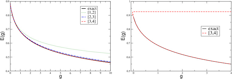
Figure 4: (color online) Left panel: Comparison between the exact integral for the zero dimensional $\phi^{4}$ theory and three different approximations obtained using the PPT; Right panel: comparison between the set $[3,4]$ and the exact integral. The approximate solution has a branch point close to $g=0$.

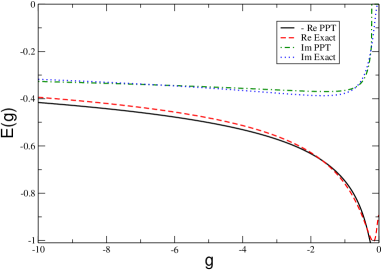
Figure 5: (color online) Real and imaginary parts of $E(g)$ for the zero dimensional $\phi^{4}$ theory obtained using the PPT with $\bar{N}=3$. The results are compared with the exact expression of eq.(22).

Let us now briefly explore a different issue. If we push forward the analogy with quantum field theory, the application of the PPT to this problem can have a simple interpretation in terms of Feynman diagrams: because applying the PAS we are expanding not in the coupling, but in a parameter $\varrho$, there is a infinite number of vertices appearing at tree level, whose couplings contain the unknown constants $c_{n}$ and $d_{n}$. The spirit of the PAS is then to perform a perturbative (in $\varrho$) calculation in which all diagrams corresponding to orders higher than $\varrho$ cancel out by fixing the unknown constants and therefore yielding the observable in terms of just two diagrams, with zero and one vertex respectively. This argument is sketched in Fig.6.

Figure 6: Feynman diagrams for the propagator in a $\phi^{4}$ theory. The diagrams with dashed line need to cancel fixing the unknown coupling contained in the bold vertex. The coulings coming from the expansion of $g$ to order $\varrho^{2}$ and higher are represented with a bold circle.

III.4 QED effective action

We consider the QED effective action in the presence of a constant background magnetic field:

$$S=-\frac{e^{2}B^{2}}{8\pi^{2}}\int_{0}^{\infty}\frac{ds}{s^{2}}\left\{\coth s-\frac{1}{s}-\frac{s}{3}\right\}\ e^{-\frac{m_{e}^{2}s}{eB}}\ ,$$ (37)

where $B$ is the magnetic field strength, $e$ the electron charge and $m_{e}$ the electron mass. Following Jent we introduce the effective coupling $g=e^{2}B^{2}/m_{e}^{2}$ and obtain the divergent perturbative series

$$S=-2\frac{e^{2}B^{2}}{\pi^{2}}g\ \sum_{n=0}^{\infty}b_{n}g^{n}$$ (38)

with

$$b_{n}=(-1)^{n+1}\frac{4^{n}|{\cal B}_{2n+4}|}{(2n+4)(2n+3)(2n+2)}\ ,$$ (39)

${\cal B}_{2n+4}$ being Bernoulli numbers.

In Fig.7 we show the comparison between the exact numerical result for $E(g)\equiv S(g)/(2\frac{e^{2}B^{2}}{\pi^{2}})$ and the approximation obtained with the set $[4,4]$: although we have used only ten perturbative coefficients, the resummation provides a quite precise approximation over a large range of the coupling in an analytical form.

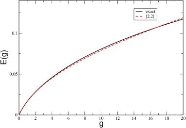
Figure 7: (Color online) Comparison between the exact numerical result for $E(g)\equiv S(g)/(2\frac{e^{2}B^{2}}{\pi^{2}})$ and the approximation obtained with the set $[4,4]$.

III.5 One plaquette integral

In LiMeu the weak coupling expansion for a one-plaquette SU(2) lattice gauge theory was discussed. The partition function in this case is given by

$$Z(\beta)=\frac{2}{\pi}\int_{-1}^{+1}\sqrt{1-u^{2}}e^{-\beta(1-u)}\ du$$ (40)

and can be calculated exactly in terms of the modified Bessel function $I_{1}$:

$$Z(\beta)=2e^{-\beta}\frac{I_{1}(\beta)}{\beta}$$ (41)

This expression admits a convergent series expansion around $\beta=0$ (strong coupling expansion), but provides a divergent series when expanded in the opposite regime, $\beta\rightarrow\infty$, (weak coupling expansion)LiMeu :

$$Z(\beta)\approx(\beta\pi)^{-3/2}2^{1/2}\sum_{l=0}^{\infty}\frac{(\Gamma(l+1/2))^{2}(l+1/2)}{l!(1/2-l)}\ .$$ (42)

The terms of this series grow like $l!/2^{l}$ and the sign does not oscillate.

We will now apply our method to this model, considering both regimes and using as usual the functional relation

$$g(\varrho)=\varrho\ \left[\frac{1+\sum_{n=1}^{\bar{N}_{u}}c_{n}\varrho^{n}}{1+\sum_{n=1}^{\bar{N}_{d}}d_{n}\varrho^{n}}\right].$$ (43)

to be determined independently in the two regimes.

III.5.1 Weak coupling expansion

In this case we identify $\beta=1/g$ and use a set corresponding to $\bar{N}_{u}=2$ and $\bar{N}_{d}=3$, obtaining the solution

$$\frac{1}{\beta}=g(\varrho)=\frac{\varrho\left(1.816\varrho^{2}-3.428\varrho+1\right)}{0.154\varrho^{3}+0.920\varrho^{2}-3.115\rho+1}$$ (44)

III.5.2 Strong coupling expansion

In this case we identify $\beta=g$ and a set corresponding to $\bar{N}_{u}=6$ and $\bar{N}_{d}=3$, obtaining the solution

$$\beta=g(\varrho)\approx\frac{\varrho\left(-0.0000545\varrho^{6}-0.000489\varrho^{5}-0.00349\varrho^{4}-0.0324\varrho^{3}+0.636\varrho^{2}-1.555\varrho+1\right)}{-0.327\varrho^{3}+1.509\varrho^{2}-2.180\varrho+1}$$ (45)

In Fig.8 we have plotted $P=-\frac{d}{d\beta}lnZ$ as a function of $\beta$, as done also in Fig.3 of LiMeu . Our results show that both the Weak and Strong coupling expansions, resummed through the PPT converge to the exact result: this is particularly remarkable in the case of the weak coupling expansion.

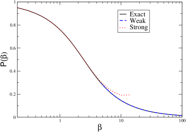
Figure 8: (color online) $P$ versus $\beta$ for SU(2) on one plaquette. The solid line is the exact result; the dashed line corresponds to the Weak Coupling Expansion; the dotted line corresponds to the Strong Coupling Expansion.

III.6 $\phi^{4}$ field theory in $1+1$

In a recent paper Nishiyama Nish01 has studied a lattice $\phi^{4}$ model in $1+1$ dimensions, described by the hamiltonian

$$\hat{H}=\sum_{i}\left[\frac{1}{2}\hat{\pi}_{i}^{2}+\hat{\phi}_{i}^{4}+g\left(\frac{1}{2}\left(\hat{\phi}_{i}-\hat{\phi}_{i+1}\right)^{2}+\frac{1}{2}\hat{\phi}_{i}^{2}\right)\right]\ ,$$ (46)

where $i$ is the site index and $\hat{\pi}_{i}$ and $\hat{\phi}_{i}$ are canonically conjugated operators. Notice that we have changed the notation in Nish01 adopting the conventions used in this paper.

Using a linked cluster expansion Nishiyama has obtained the perturbation series in $g$ up to order 11:

$$E(g) = 0.66798625915577710827096201688+0.43100635014259473006095738275g$$ (47)

$$- 0.10148809521111863294125944502g^{2}+0.04803845646443637442034775341g^{3}$$

$$- 0.029018513979643624653232757064g^{4}+0.019777791330895673863274529570g^{5}$$

$$- 0.014454753622894705466341917665g^{6}+0.01106139124598227911409431586g^{7}$$

$$- 0.0087493465269972g^{8}+0.007096747591805g^{9}-0.005871428g^{10}+0.00493622g^{11}\ .$$

Since the perturbative series has a radius of convergence $g_{0}\approx 1$, an Aitken $\delta^{2}$ process was used in Nish01 to accelerate the convergence of this series. The accelerated series was then compared with the numerical results obtained using the Density Matrix Renormalization Group (DMRG), showing that the region of convergence could be enlarged up to $g\approx 2$.

We will now apply our method to this problem and consider

$$g(\varrho)=\varrho\ \left[\frac{1+\sum_{n=1}^{\bar{N}_{u}}c_{n}\varrho^{n}}{1+\sum_{n=1}^{\bar{N}_{d}}d_{n}\varrho^{n}}\right],$$ (48)

where as usual $N_{u}$ and $N_{d}$ fix the asymptotic behavior for $g\rightarrow\infty$. As we do not know this behavior exactly we will work at order $N_{u}+N_{d}=5$ and take into account all the possible combinations of $\bar{N}_{u}$ and $\bar{N}_{d}$ keeping the sum fixed. In this case only the coefficients $b_{n}$ with $n$ going from 0 to 6 are used, the remaining being a prediction of our method. In Fig.9 we have plotted the difference between the perturbative polynomial of order $g^{11}$ given by Nishiyama and the polynomial of order $g^{11}$ constructed with PPT working to order $N_{u}+N_{d}=5$. As one can see, the set $[3,2]$ provides the smallest difference, a result which suggests the asymptotic behavior of the energy as $E\propto\sqrt{g}$ for $g\rightarrow\infty$.

In Table 3 we have compared the exact coefficients calculated by Nishiyama with those predicted by the PPT working with the set $[3,2]$. The last row of this table shows the errors $\Sigma_{n}\equiv 100\times\left|b_{n}^{[3,2]}/b_{n}^{exact}-1\right|$: from this results we can conclude that resummation through PPT allows to achieve a truly remarkable precision, the largest error being of about $0.1\%$.

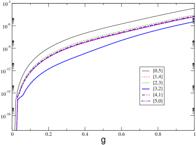
Figure 9: (color online) Difference between the perturbative polynomial of order $g^{11}$ given by Nishiyama and the polynomial of order $g^{11}$ constructed with PPT working to order $N_{u}+N_{d}=5$.

Table 3: Comparison between the perturbative coefficients of Nish01 and those predicted with PPT working with the set $[3,2]$.

	$b_{7}$	$b_{8}$	$b_{9}$	$b_{10}$	$b_{11}$
$b_{n}^{exact}$	0.011061391245982	-0.0087493465269972	0.007096747591805	-0.005871428	0.00493622
$b_{n}^{[3,2]}$	0.011061133480144	-0.0087483769472128	0.007094602847397	-0.00586767	0.00493037
error ($\%$)	0.00233	0.011081739435	0.03022	0.06403	0.11851

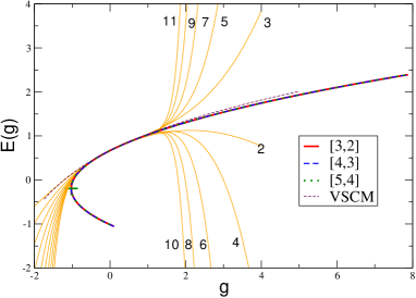
Figure 10: (color online) Comparison between the resummed energies to orders $[3,2]$, $[4,3]$ and $[5,4]$ and the perturbative polynomials.

In Fig.10 we have compared the perturbative polynomials for the energy from orders $g^{2}$ to $g^{11}$ with the energy resummed with the sets $[3,2]$, $[4,3]$ and $[5,4]$. There are several striking aspects which should impress the reader: first of all, the difference bewteen the three sets is extremely thiny, thus signaling that the convergence is extremely strong; in second place, the resummed energy confirms the DMRG result displayed in Fig.2 of Nish01 ; finally, the resummed energy is a multivalued function, with a branch point at $g\approx-1.025$. This last finding is extremely interesting, because in Nish01 it was speculated the existence of a phase transition at $g\approx-2$ (in our notation): the resummed energy plotted in Fig.2 of Nish01 appears to have a singularity around $g=-1$ (in our notation), i.e. in the same region where we observe the branch point . Because of the use of a parameter $\varrho$, PPT can deal with multivalued functions in a way which is not possible in conventional perturbation theory. Finally, the thiny dashed line in the plot corresponds to the numerical result obtained in Amore06a using the Variational Sinc Collocation Method (VSCM) within a mean field approach.

III.7 Elastic theory

Another example of divergent series has been studied in Buch96 . The authors of that paper have found out that the series for the inverse bulk modulus $K$ as a function of the compression:

$$\frac{1}{K}=b_{0}+b_{1}P+b_{2}P^{2}+\dots$$ (49)

has zero radius of convergence and they obtained an explicit expression for the coefficients in a simplified calculation. In the following we will uniform the notation to the conventions used in this paper and refer to the pressure $P$ as the coupling $g$. The coefficients of the series are Buch96

$$b_{n}=-(n+2)\frac{f_{n+2}}{A}$$ (50)

where

$$f_{n}=(-1)^{n+1}\ \Gamma\left(\frac{n+1}{2}\right)\ \left(\frac{\pi\sqrt{1-\sigma^{2}}}{4\beta Y\alpha^{2}}\right)^{n/2}\ \left(\frac{2\pi A}{\lambda^{2}}\right)\ \frac{\sqrt{1-\sigma^{2}}}{2\sqrt{\pi}\beta^{5/2}\alpha\lambda^{2}\sqrt{Y}}\ .$$ (51)

Here $\alpha$ is the surface tension, $Y$ is the Young’s modulus, $\sigma$ is the Poisson ratio, $\beta=1/k_{B}T$ and $\lambda$ is the ultraviolet cutoff of the theory. To apply our method we introduce

$$g(\varrho)=\varrho\ \frac{1+\sum_{n=1}^{\bar{N}_{u}}c_{n}\varrho^{n}}{1+\sum_{n=1}^{\bar{N}_{d}}d_{n}\varrho^{n}}$$ (52)

and fix $\bar{N}_{u}+\bar{N}_{d}=5$. Working to this order the first predicted coefficient is $b_{7}$. We have performed a calculation using $\beta=\lambda=\alpha=Y=1$ and $\sigma=1/2$.

Table 4: Comparison of the exact perturbative coefficient $b_{7}$ for the elastic series with the approximate coefficient predicted by PPT using $\bar{N}_{u}+\bar{N}_{d}=5$. $b_{7}^{exact}=-\frac{729\pi^{5}}{8192}\approx-27.2324646250573949498$. The parameters are chosen $\beta=\lambda=\alpha=Y=1$ and $\sigma=1/2$.

	$b_{7}^{[5,0]}$	$b_{7}^{[4,1]}$	$b_{7}^{[3,2]}$	$b_{7}^{[2,3]}$	$b_{7}^{[1,4]}$	$b_{7}^{[0,5]}$
$b_{7}$	-48.40832399	-27.41931538	-27.18605118	-27.21965479	-27.17382665	-27.46859099
error ($\%$)	$77.75$	$0.69$	$0.17$	$0.047$	$0.21$	$0.87$

As we have seen from Table 4 the optimal set for $\bar{N}_{u}+\bar{N}_{d}$ is $[2,3]$, corresponding to an asymptotic behavior $1/K\propto g^{0}$. At this order we have found :

$$g(\varrho)=\frac{\varrho\left(-0.4923950887\varrho^{2}-0.94207053700\varrho+1\right)}{0.6331671415\varrho^{3}+0.9634343699\varrho^{2}-2.4724637506\varrho+1}$$ (53)

Working with to order $\bar{N}_{u}+\bar{N}_{d}=7$ we have found that the best set is the $[5,2]$, which provides a different asymptotic behavior for the inverse compression modulus, $1/K\propto g^{1/4}$. In Table 5 we compare the predictions for the perturbative coefficients obtained with the two different sets: notice that the second set does not predict the coefficients $b_{7}$ and $b_{8}$. The second set gives more precise results than the first set for $b_{9}$ and $b_{10}$, but a slightly worse error for $b_{11}$.

In Fig.11 we have compared the perturbative polynomials of order $8$ through $10$ with PPT results corresponding to the sets $[2,3]$,$[5,2]$ and $[6,6]$: just as in the case of the lattice $\phi^{4}$ previously discussed we observe a branch point in the resummed solution, corresponding to $g_{0}^{[2,3]}\approx-0.412879$, $g_{0}^{[5,2]}\approx-0.401549$ and $g_{0}^{[6,6]}\approx-0.330171$ with the different sets.

If we go back to the example of $\phi^{4}$ in zero dimensions, there we have seen that $g=0$ is a point where the function is not analytical and therefore the perturbative series is divergent. In the present example we can use the words of the authors of Buch96 and say that “under stretching ($g<0$) the true ground state is fractured into pieces. As a result $g=0$ cannot be a point of analyticity for $K(g)$ and thus the series has zero radius of convergence”. Our results however display a branch point not exactly at $g=0$ or close to it as in the case of the $\phi^{4}$ model in zero dimensions.

Table 5: Comparison between the perturbative coefficients of Buch96 and those predicted with PPT working with the set $[2,3]$. We use $\beta=\lambda=\alpha=Y=1$ and $\sigma=1/2$. Coefficients with a dagger are input of the method.

	$b_{7}$	$b_{8}$	$b_{9}$	$b_{10}$	$b_{11}$
$b_{n}^{exact}$	- 27.2324646250574	51.2814820354647	- 100.257786099872	203.060091610056	-425.208317773323
$b_{n}^{[2,3]}$	- 27.2196547938467	51.1255824090448	- 99.224725761445	197.961957448658	-561.00565159656
error ($\%$)	0.047	0.304	1.03	2.51	31.9
$b_{n}^{[5,2]}$	- 27.2324646250574†	51.2814820354647†	-100.216793832003	202.536703574420	-579.771361475677
error ($\%$)	0	0	0.041	0.26	36.35

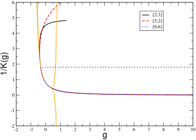
Figure 11: (color online) Comparison between the perturbative polynomials of order $8$ through $10$ and the results obtained using the sets $[2,3]$ and $[5,2]$ with PPT .

III.8 Elliptic integral of the first kind

Consider the elliptic integral of the first kind:

$$E(g)=K(g)\equiv\int_{0}^{\pi/2}\frac{dt}{\sqrt{1-g\sin^{2}t}}\ ,$$ (54)

which diverges for $g\rightarrow 1$. It also obeys the series representation

$$K(g)=\frac{\pi}{2}\sum_{k=0}^{\infty}\frac{\left(\frac{1}{2}\right)_{k}\left(\frac{1}{2}\right)_{k}}{k!^{2}}g^{k}$$ (55)

which converges for $|g|<1$.

We want to show that it is possible to resum the perturbative series using the PPT. We choose the functional form:

$$g(\varrho)=\varrho\ \frac{1+\sum_{n=1}^{\bar{N}}c_{n}\varrho^{n}}{1+\sum_{n=1}^{\bar{N}+1}d_{n}\varrho^{n}}\ .$$ (56)

The choice of $\bar{N}_{u}+1=\bar{N}_{d}$ is not arbitrary: with this choice we have that $\lim_{\varrho\rightarrow\infty}g(\varrho)=\bar{g}<\infty$, which means that the resummed function will have a singularity precisely at $g=\bar{g}$.

Using $\bar{N}=2$ we find

$$g(\varrho)=\frac{\varrho\left(\frac{381\varrho^{2}}{35840}+\frac{187\varrho}{2240}+1\right)}{\frac{2301\varrho^{3}}{286720}+\frac{1181\varrho^{2}}{8960}+\frac{1447\varrho}{2240}+1}$$ (57)

which predicts the singularity of the elliptic integral at

$$\bar{g}^{[2,3]}=\frac{1016}{767}\approx 1.324\ .$$ (58)

Increasing $\bar{N}$ this singularity moves towards its exact value, $\bar{g}=1$; for example, using $\bar{N}=3,4$ and $5$ and find

$$\bar{g}^{[3,4]}=\frac{4999}{3752}\approx 1.332\ ,\ \bar{g}^{[4,5]}=\frac{5509}{8216}\approx 0.670\ ,\ \bar{g}^{[5,6]}=\frac{69944792}{67596985}\approx 1.035\ .$$ (59)

The reader will notice that the singularity predicted by the set $[4,5]$ falls below the exact singularity: the reason for this behavior is easily understood looking at Fig.12. As a matter of fact the set $[4,5]$ (the thin line in the plot) has a branch point close to $g=1$, and therefore the singularity belongs to the nonphysical branch. Notice that the set $[5,6]$ provides an excellent approximation.

Let us now compare the expansion of $K(g)^{[2,3]}$ around $g=0$ with the exact result, provided by the series (55). We have

$$K(g)^{[2,3]} \approx \frac{\pi}{2}+\frac{\pi g}{8}+\frac{9\pi g^{2}}{128}+\frac{25\pi g^{3}}{512}+\frac{1225\pi g^{4}}{32768}+\frac{3969\pi g^{5}}{131072}+\frac{53361\pi g^{6}}{2097152}+\frac{206126367\pi g^{7}}{9395240960}$$ (60)

$$+ \frac{405813405891\pi g^{8}}{21045339750400}+\frac{810831328918663\pi g^{9}}{47141561040896000}+\frac{1639189758117069059\pi g^{10}}{105597096731607040000}$$

$$+ \frac{3345592829494380888687\pi g^{11}}{236537496678799769600000}+\frac{6882636481373124653844491\pi g^{12}}{529843992560511483904000000}+\dots$$

$$\approx 1.5707963267949+0.392699081698724g+0.220893233455532g^{2}+0.153398078788564g^{3}$$

$$+ 0.117445404072494g^{4}+0.09513077729872g^{5}+0.079936278146842g^{6}+0.06892479746239g^{7}$$

$$+ 0.060578751866013g^{8}+0.054035158997418g^{9}+0.0487671220263656g^{10}$$

$$+ 0.0444347725101475g^{11}+0.0408090692936214g^{12}+\dots$$

and

$$K(g) \approx \frac{\pi}{2}+\frac{\pi g}{8}+\frac{9\pi g^{2}}{128}+\frac{25\pi g^{3}}{512}+\frac{1225\pi g^{4}}{32768}+\frac{3969\pi g^{5}}{131072}+\frac{53361\pi g^{6}}{2097152}+\frac{184041\pi g^{7}}{8388608}$$ (61)

$$+ \frac{41409225\pi g^{8}}{2147483648}+\frac{147744025\pi g^{9}}{8589934592}+\frac{2133423721\pi g^{10}}{137438953472}+\frac{7775536041\pi g^{11}}{549755813888}+\frac{457028729521\pi g^{12}}{35184372088832}+\dots$$

$$\approx 1.5707963267949+0.392699081698724g+0.220893233455532g^{2}+0.153398078788564g^{3}$$

$$+ 0.117445404072494g^{4}+0.0951307772987205g^{5}+0.0799362781468415g^{6}+0.0689246479939603g^{7}$$

$$+ 0.0605783039009417g^{8}+0.0540343513190498g^{9}+0.0487660020654424g^{10}$$

$$+ 0.0444334853530168g^{11}+0.0408078363745588g^{12}+\dots\ .$$

Notice that coefficients starting from $7$ and higher, are predictions of the PPT: we see, for example, that the coefficient of the term of order $g^{12}$ is predicted with an error $0.003\%$!

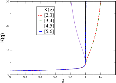
Figure 12: (color online) Comparison between elliptic integral $K(g)$ and the PPT approximations obtained with sets $[2,3]$, $[3,4]$, $[4,5]$ and $[5,6]$.

III.9 Virial coefficients

As a last example we consider the low density virial expansion of the pressure

$$\frac{P}{k_{B}T}=\sum_{n=1}^{\infty}B_{k}\rho^{k}\ ,$$ (62)

where the $B_{k}$ are the virial coefficients and $\rho$ is the density (not to be confused with $\varrho$). Table 1 of Clis06 contains the numerical values of the virial coefficients for hard spheres in $D$ dimensions, with $2\leq D\leq 8$. In the following we will uniform the notation in (62) to the notation adopted in this paper and call $g$ the density.

As usual we adopt the functional form

$$g(\varrho)=\varrho\ \frac{1+\sum_{n=1}^{\bar{N}_{u}}c_{n}\varrho^{n}}{1+\sum_{n=1}^{\bar{N}_{d}}d_{n}\varrho^{n}}\ .$$ (63)

In Table 6 we have used PPT with $\bar{N}_{u}+\bar{N_{d}}=5$ to predict the virial coefficients $B_{9}$ and $B_{10}$ from the previous one. As one can see the set $[2,3]$ provides highly precise results. We have then used the set $[3,4]$ which has the same behaviour for $\varrho\rightarrow\infty$ to obtain an estimate for the eleventh virial coefficient. To orders $[2,3]$ and $[3,4]$ we have found

$$\left[B_{11}/B_{2}^{10}\right]^{[2,3]}=0.01094432\ \ \ ,\ \ \ \left[B_{11}/B_{2}^{10}\right]^{[3,4]}=0.01090061\ .$$ (64)

Since these results are not (yet) available in the literature, the prediction made here will be a strong test of the present method once the calculation of $B_{11}$ will be made. In Table 7 we compare our predictions for the virial coefficients going from $B_{11}$ to $B_{18}$ with the predictions made in Clis06 . Our predictions are very close to those made by Clisby and McCoy for $D=2$.

Notice that finding $N_{u}+1=N_{d}$ has an important effect: as discussed in the previous example of the elliptic integral, in this case the solution will have a singularity at a finite value of $g$. For example, if we consider the set $[3,4]$ the tranformation reads

$$g(\varrho)=\frac{\varrho\left(0.3004\varrho^{3}+1.8876\varrho^{2}+2.7141\varrho+1\right)}{0.2584\varrho^{4}+2.1266\varrho^{3}+4.6986\varrho^{2}+3.7831\varrho+1}$$ (65)

and the singularity is predicted to be fall at

$$\bar{g}^{[3,4]} = \lim_{\varrho\rightarrow\infty}g(\varrho)\approx 1.1625.$$ (66)

We would like to stress that this singularity is “physical”, i.e. it is a singularity of the resummed function, in contrast with the singularity falling at the radius of convergence of a series. We can use the previous example of the elliptic integral to better understand this point: in that case the perturbative series around $g=0$ had a radius of convergence $1$, coinciding with the location of the true singularity of $K(g)$.

If we trust our result, we may conclude that the $\frac{P}{k_{B}T}$ becomes infinite at a finite density $g\approx\bar{g}^{[3,4]}$.

We have also considered the virial series in $D=3$ dimensions. Also in this case we have found out that, working with $\bar{N}_{u}+\bar{N}_{d}=5$ the optimal set corresponds to $[2,3]$ (see Table 6) and therefore the virial series is expected to have a singularity at finite density:

$$\bar{g}^{[3,4]} = \lim_{\varrho\rightarrow\infty}g(\varrho)\approx 1.43439\ .$$ (67)

In Table 7 we have also compared our predictions obtained with the set $[3,4]$ for $D=3$ with those made in Clis06 . Unlike in the previous case, our result agree to some extent with those of Clis06 only for the coefficient $B_{11}$, whereas completely different predictions are made for the remaining coefficients.

Table 6: Virial coefficients for a hard spheres in $2$ and $3$ dimensions given in Table I of Clis06 and predictions using PPT with different sets.

	$B_{9}/B_{2}^{8}$	$B_{10}/B_{2}^{9}$	$B_{9}/B_{2}^{8}$	$B_{10}/B_{2}^{9}$
	$D=2$		$D=3$
Ref.Clis06	$0.0362193$	$0.0199537$	$0.0013094$	$0.0004035$
$[0,5]$	$0.03739998$	$0.02496595$	$0.0023400$	$0.0031580$
$[1,4]$	$0.03625994$	$0.02008503$	$0.0013509$	$0.0004884$
$[2,3]$	$0.0362321$	$0.0199843$	$0.0013165$	$0.0004198$
$[3,2]$	$0.0362551$	$0.02006717$	$0.0013404$	$0.0004664$
$[4,1]$	$0.0368599$	$0.02258546$	$0.0017325$	$0.0014442$
$[5,0]$	$0.1747048$	$0.75984885$	$0.0222648$	$0.0735264$

Table 7: Predicted coefficients for approximants with 10 exact coefficients for $D=2$ and $D=3$. Comparison between the predictions of Clis06 and the predictions obtained using the set $[3,4]$.

	$B_{11}/B_{2}^{10}$	$B_{12}/B_{2}^{11}$	$B_{13}/B_{2}^{12}$	$B_{14}/B_{2}^{13}$	$B_{15}/B_{2}^{14}$	$B_{16}/B_{2}^{15}$	$B_{17}/B_{2}^{16}$	$B_{18}/B_{2}^{17}$
$D=2$
Ref.Clis06	$1.089\times 10^{-2}$	$5.90\times 10^{-3}$	$3.18\times 10^{-3}$	$1.70\times 10^{-3}$	$9.10\times 10^{-4}$	$4.84\times 10^{-4}$	$2.56\times 10^{-4}$	$1.36\times 10^{-4}$
$[3,4]$	$1.0901\times 10^{-2}$	$5.9235\times 10^{-3}$	$3.2117\times 10^{-3}$	$1.7421\times 10^{-3}$	$9.4698\times 10^{-4}$	$5.1638\times 10^{-4}$	$2.8247\times 10^{-4}$	$1.5492\times 10^{-4}$
$D=3$
Ref.Clis06	$1.22\times 10^{-4}$	$3.64\times 10^{-5}$	$1.08\times 10^{-5}$	$3.2\times 10^{-6}$	$9.2\times 10^{-7}$	$2.6\times 10^{-7}$
$[3,4]$	$1.1599\times 10^{-4}$	$2.2229\times 10^{-5}$	$-8.5616\times 10^{-6}$	$-1.8088\times 10^{-5}$	$-2.0325\times 10^{-5}$	$-2.0112\times 10^{-5}$	$-1.9136\times 10^{-5}$	$-1.7971\times 10^{-5}$

IV Conclusions

We have developed a new method, Parametric Perturbation Theory (PPT), which is alternative to the ordinary perturbation theory, i.e. does not amount to an expansion in any physical parameter. We have shown that PPT can used either as a fully autonomous perturbation scheme, as done in Section II, or it can be applied to the coefficients of the perturbative expansion, resumming the series and providing physically meaningful results, as done in Section III. There are several aspects of our method which should make it very appealing:

• since PPT can use perturbative results as an input, it can be applied with limited effort to the huge amount of problems which have been studied perturbatively;

• it provides analytical approximations;

• unlike variational methods, such as the LDE or VPT, our method does not require any optimization in a variational parameter;

• although the asymptotic (strong coupling) behavior of the solution can be used, when known, to refine the functional relation $g=g(\varrho)$, PPT is capable of selecting the most appropriate asymptotic behavior of the solution within a class of different behaviors allowed to a given order;

• it predicts the unknown perturbative coefficients with high precision;

• it can easily describe multivalued functions and therefore is capable to produce branch points at finite order, as observed in the examples: if these points are related to phase transitions of a system, as claimed in Nish01 in the case of $\phi^{4}$ in $1+1$, then our method could provide an alternative tool to the study of critical phenomena;

• it can produce singularities in an observable working at finite order, as seen for the cases of the elliptic integral of first kind and for the virial coefficients of a hard sphere gas;

• most importantly, it can produce the nonperturbative imaginary part of an observable, which appears when a system becomes metastable.

Future directions of work will certainly include the development of an autonomous perturbation scheme for quantum mechanical problems, in analogy to the one developed in classical mechanics and the application of our results to resum perturbative calculations in quantum field theory. It will be also interesting to apply PPT to obtain new analytical approximations for special functions of relevance in Physics, as done in this paper with the elliptic integral of the first kind.

References

- (1) F.M.Fernández, Introduction to Perturbation Theory in quantum mechanics, CRC, Boca Raton (2001);
- (2) G. A. Arteca, F. M. Fernández, and E. A. Castro, Large order perturbation theory and summation methods in quantum mechanics Springer (1990);
- (3) E.J.Hinch, Perturbation methods, Cambridge University Press (2002);
- (4) A.H.Nayfeh, Perturbation methods, J.Wiley and sons, New York (2000)
- (5) F. Dyson, Phys.Rev. 85, 631-632 (1952)
- (6) C. Bender and T.T.Wu, Phys.Rev.184, 1231-1260 (1969)
- (7) C.M. Bender and S.A.Orszag, Advanced Mathematical Methods for Scientists and Engineers, McGraw-Hill, New York, 1978
- (8) E.J.Weniger, Comp.Phys.Rep.10, 189 (1989)
- (9) A. Okopińska, Phys. Rev. D 35, 1835 (1987); A. Duncan and M. Moshe, Phys. Lett. B 215, 352 (1988)
- (10) H. Kleinert, Path Integrals in Quantum Mechanics, Statistics and Polymer Physics, 3rd edition (World Scientific Publishing, 2004)
- (11) P.M. Stevenson, Phys. Rev. D 23, 2916 (1981)
- (12) P.Amore and A.Aranda, Phys.Lett. A 316, 218-225 (2003)
- (13) P.Amore and N.Sanchez, J. Sound and Vibration 300, 345-351 (2007)
- (14) J.J.Loeffel,A. Martin, B.Simon and A.S.Wightman, Phys.Lett. B 30, 656-658 (1969)
- (15) E.J.Weniger, J.Cizek and F.Vinette, J. Math. Phys. 34, 571(93)
- (16) I.A.Ivanov, Phys.Rev. A 54, 81-86 (1995)
- (17) E.J.Weniger, Phys.Rev.Lett.77, 2859-2862 (1996)
- (18) J.Cizek, E.J.Weniger, P.Bracken and V.Spirko, Phys. Rev. E 53, 2925-2939 (1996)
- (19) A.V. Sergeev and D.Z. Goodson, J.Phys. A 31, 4301-4317 (1998)
- (20) H.H. Homeier, Acta Applicandae Mathematicae 61, 133-147 (2000)
- (21) M.A. Nuñez, Phys.Rev.E 68, 016703 (2003)
- (22) D.Roy and R.Bhattacharya, Annals of Physics 321, 1483-1523 (2006)
- (23) H. Kleinert and W.Janke, Phys. Rev.Lett. 75, 2787-2791 (1995)
- (24) F.M.Fernández and R. Guardiola, J.Phys.A 30, 7187-7192 (1997)
- (25) C.M.Bender and G.V. Dunne, J. Math. Phys.40, 4616-4621 (1998)
- (26) C.M.Bender and E.J.Weniger, J. Math. Phys.42, 2167-2183 (2001)
- (27) J.Zinn-Justin, Quantum Field Theory and Critical Phenomena, Clerendon Press-Oxford, New York (2002)
- (28) I.R.C.Buckley, A. Duncan and H.F.Jones, Phys.Rev.D 47, 2554-2559 (1993)
- (29) C.M.Bender, A. Duncan and H.F.Jones, Phys.Rev.D 49, 4219-4225
- (30) U. D. Jentschura, J. Becher, E. J. Weniger and G. Soff, Phys. Rev. Lett. 85, 2446 (2000)
- (31) L.Li and Y.Meurice, Phys.Rev. D 71, 054509 (2005)
- (32) Y. Nishiyama, J.Phys.A 34, 11215-11223 (2001)
- (33) P.Amore, J.Phys.A L349-L355 (2006)
- (34) A. Buchel and J.P.Sethna, Phys. Rev.Lett. 77, 1520-1523 (1996)
- (35) N.Clisby and B. McCoy, Jour. of Stat. Phys. 122 15-57 (2006)