FRUSTRATION EFFECTS IN ANTIFERROMAGNETIC FCC HEISENBERG FILMS

Abstract

We study the effects of frustration in an antiferromagnetic film of FCC lattice with Heisenberg spin model including an Ising-like anisotropy. Monte Carlo (MC) simulations have been used to study thermodynamic properties of the film. We show that the presence of the surface reduces the ground state (GS) degeneracy found in the bulk. The GS is shown to depend on the surface in-plane interaction $J_{s}$ with a critical value at which ordering of type I coexists with ordering of type II. Near this value a reentrant phase is found. Various physical quantities such as layer magnetizations and layer susceptibilities are shown and discussed. The nature of the phase transition is also studied by histogram technique. We have also used the Green’s function (GF) method for the quantum counterpart model. The results at low-$T$ show interesting effects of quantum fluctuations. Results obtained by the GF method at high $T$ are compared to those of MC simulations. A good agreement is observed.

I Introduction

Effects of the frustration in spin systems have been extensively investigated during the last 30 years. Frustrated spin systems are shown to have unusual properties such as large ground state (GS) degeneracy, additional GS symmetries, successive phase transitions with complicated nature. Frustrated systems still challenge theoretical and experimental methods. For recent reviews, the reader is referred to Ref. Diep2005, .

On the other hand, during the same period physics of surfaces and objects of nanometric size have also attracted an immense interest. This is due to important applications in industry.zangwill ; bland-heinrich ; Binder-surf ; Diehl In this field, results from laboratory research are often immediately used for industrial applications, without waiting for a full theoretical understanding. An example is the so-called giant magneto-resistance (GMR) used in data storage devices, magnetic sensors, … Baibich ; Grunberg ; Fert ; review In parallel to these experimental developments, much theoretical effort has also been devoted to the search of physical mechanisms lying behind new properties found in nanometric objects such as ultrathin films, ultrafine particles, quantum dots, spintronic devices etc. This effort aimed not only at providing explanations for experimental observations but also at predicting new effects for future experiments.ngo2004trilayer ; ngo2007

The aim of this paper is to investigate the effect of the presence of a film surface in a system which is known to be very frustrated, namely the FCC antiferromagnet. The bulk properties of this material have been largely studied as we will show below. In this paper, we would like to see in particular how the frustration effects on the nature of the phase transition in 3D are modified in thin films and how the surface conditions affect the magnetic phase diagram. To carry out these purposes, we shall use Monte Carlo (MC) simulations and the Green’s function (GF) method for qualitative comparison.

The paper is organized as follows. Section II is devoted to the description of the model. We recall there properties of the 3D counterpart model in order to better appreciate properties of thin films obtained in this paper. A determination of its GS properties is also given. In section III, we show our results obtained by MC simulations as functions of temperature $T$. The surface exchange interaction $J_{s}$ is made to vary. A phase diagram in the space $(T,J_{s})$ is shown and discussed. In general, the surface transition is found to be distinct from the transition of interior layers. An interesting reentrant region is observed in the phase diagram. We also show in this section the results on the critical exponents obtained by MC multihistogram technique. A detailed discussion on the nature of the phase transition is given. Section IV is devoted to a study of the quantum version of the same model by the use of the GF method. We find interesting effects of quantum fluctuations at low $T$. The phase diagram $(T,J_{s})$ is established and compared to that obtained by MC simulations for the classical model. Concluding remarks are given in section V.

II Model and Classical Ground State Analysis

It is known that the antiferromagnetic (AF) interaction between nearest-neighbor (NN) spins on the FCC lattice causes a very strong frustration. This is due to the fact that the FCC lattice is composed of corner-sharing tetrahedra each of which has four equilateral triangles. It is well-knownDiep2005 that it is impossible to fully satisfy simultaneously the three AF bond interactions on each triangle.

The analytical determination of the GS of systems of classical spins with competing interactions is a fascinating subject. For a recent review, the reader is referred to Ref. Kaplan, . For the bulk FCC antiferromagnet, the Heisenberg spins on a tetrahedron form a configuration characterized by two arbitrary angles.Oguchi The ground state (GS) degeneracy is therefore infinite. This is also found in fully frustrated simple cubic lattice with classical Heisenberg spins:Lallemand1985ff the GS is also characterized by two random continuous parameters. To give an idea about the GS of the bulk FCC antiferromagnet,Oguchi let us imagine two planes, $xz$ and $\psi$, where $\psi$ intersects with the $xz$ plane along the $z$ axis and makes an angle $\phi$ with the $x$ axis. Two of the four spins make an angle $\theta$ in the $xz$ plane symmetric with respect to the $z$ axis. The other two spins make also the same angle, symmetric with respect to the $z$ axis, but in the plane $\psi$. It has been shownOguchi that the two angles $\theta$ and $\phi$ are arbitrary between 0 and $\pi$. Note that when $\theta=0$ the spin configuration is collinear with two spins along the $+z$ axis and the other two along the $-z$ one. The phase transition of the bulk frustrated FCC Heisenberg antiferromagnet has been studied.Diep1989fcc In particular, the transition is found to be of the first order as in the Ising case.Phani ; Polgreen ; Styer Other similar frustrated antiferromagnets such as the HCP antiferromagnet show the same behavior.Diep1992hcp

Let us consider a film of FCC lattice structure with (001) surfaces. To avoid the absence of long-range order of isotropic non Ising spin model at finite temperature ($T$) when the film thickness is very small, i.e. quasi two-dimensional systemMermin , we add in the Hamiltonian an Ising-like uniaxial anisotropy term. The Hamiltonian is given by

$$\mathcal{H}=-\sum_{\left<i,j\right>}J_{i,j}\mathbf{S}_{i}\cdot\mathbf{S}_{j}-\sum_{<i>}D_{i}(S^{z}_{i})^{2}$$ (1)

where $\mathbf{S}_{i}$ is the Heisenberg spin at the lattice site $i$, $\sum_{\left<i,j\right>}$ indicates the sum over the NN spin pairs $\mathbf{S}_{i}$ and $\mathbf{S}_{j}$.

In the following, the interaction between two NN surface spins is denoted by $J_{s}$, while all other interactions are supposed to be antiferromagnetic and all equal to $J=-1$ for simplicity.

We first determine the GS configuration by using the steepest descent method : starting from a random spin configuration, we calculate the magnetic local field at each site and align the spin of the site in its local field. In doing so for all spins and repeat until the convergence is reached, we obtain easily the GS configuration without metastable states. The result is shown in Fig. 1

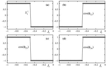
Figure 1: A ground state configuration of single plaquette (a) $S^{z}_{1}$ is $S^{z}$ of sublattice 1, (b) $\cos\theta_{12}$, (c) $\cos\theta_{23}$, (d) $\cos\theta_{34}$. $\cos\theta_{ij}$ is cosine of angle between the two spins of sublattices $i$ and $j$.

We observe that there is a critical value $J^{c}_{s}=-0.5$. For $J_{s}<J^{c}_{s}$, the spins in each $yz$ plane are parallel while spins in adjacent $yz$ planes are antiparallel (Fig. 2a). This ordering will be called hereafter ”ordering of type I”: in the $x$ direction the ferromagnetic planes are antiferromagnetically coupled as shown in this figure. Of course, there is a degenerate configuration where the ferromagnetic planes are antiferromagnetically ordered in the $y$ direction. Note that the surface layer has an AF ordering for both configurations. The degeneracy of type I is therefore 4 including the reversal of all spins.

For $J_{s}>J^{c}_{s}$, the spins in each $xy$ plane is ferromagnetic. The adjacent $xy$ planes have an AF ordering in the $z$ direction perpendicular to the film surface. This will be called hereafter ”ordering of type II”. Note that the surface layer is then ferromagnetic (Fig. 2b). The degeneracy of type II is 2 due to the reversal of all spins.

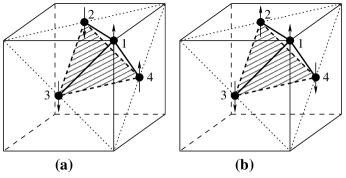
Figure 2: The ground state spin configuration of the FCC cell at the film surface: a) ordering of type I for $J_{s}<-0.5$ b) ordering of type II for $J_{s}>-0.5$.

Without using a general method,Kaplan ; Oguchi let us calculate analytically the GS configuration in a simple manner for the present model.

Consider a tetrahedron with the spins numbered as in Fig. 2: $S_{1}$, $S_{2}$, $S_{3}$ and $S_{4}$ are the spins in the surface FCC cell (first cell). The interaction between $S_{1}$ and $S_{2}$ is set to be equal to $J_{s}$ $(-1\leq J_{s}\leq 0)$ and all others are taken to be equal to $J$ ($<0$), and all $D_{i}=D$ for simplicity. The Hamiltonian for the cell is written as

$$H_{p} = -\frac{1}{2}\Big{\{}8J_{s}(\mathbf{S}_{1}\cdot\mathbf{S}_{2})+8J(\mathbf{S}_{3}\cdot\mathbf{S}_{4})$$ (2)

$$+ 6J\left[\mathbf{S}_{1}\cdot\mathbf{S}_{3}+\mathbf{S}_{1}\cdot\mathbf{S}_{4}+\mathbf{S}_{2}\cdot\mathbf{S}_{3}+\mathbf{S}_{2}\cdot\mathbf{S}_{4}\right]$$

$$+ 2D\left[(S^{z}_{1})^{2}+(S^{z}_{2})^{2}+(S^{z}_{3})^{2}+(S^{z}_{4})^{2}\right]\Big{\}}.$$

Let us decompose each spin into two components: an $xy$ component, which is a vector, and a $z$ component $\mathbf{S}_{i}=(\mathbf{S}_{i}^{\parallel},S_{i}^{z})$. The numerical results shown above indicate that the spins have only $z$ component. Taking advantage of this, we suppose that the $xy$ vector components of the spins are all equal to zero. The angles $\theta_{i}$ of $\mathbf{S}_{i}$ with the $z$ axis are then

$$\left\{\begin{array}[]{ll}\theta_{1}=0,&\theta_{3}=\pi\\ \theta_{2}=\beta_{1},&\theta_{4}=\beta_{2}.\end{array}\right.$$

The total energy of the cell (2), with $S_{i}=\frac{1}{2}$, can be rewritten as

$$H_{p} = -\frac{D}{2}+\frac{3J}{4}+\left(\frac{3J}{4}-J_{s}-\frac{D}{4}\cos\beta_{1}\right)\cos\beta_{1}$$ (3)

$$+ \frac{1}{4}\left(J-D\cos\beta_{2}\right)\cos\beta_{2}-\frac{3J}{4}\cos\beta_{1}\cos\beta_{2}.$$

By a variational method, the minimum of the cell energy corresponds to

$$\frac{\partial H_{p}}{\partial\beta_{1}} = J_{s}\sin\beta_{1}+\frac{D}{2}\cos\beta_{1}\sin\beta_{1}$$ (4)

$$- \frac{3J}{4}\sin\beta_{1}+\frac{3J}{4}\cos\beta_{2}\sin\beta_{1}=0,$$

$$\frac{\partial H_{p}}{\partial\beta_{2}} = \left[\frac{3J}{4}\cos\beta_{1}-\frac{J}{4}+\frac{D}{2}\cos\beta_{2}\right]\sin\beta_{2}=0.$$ (5)

The solutions of Eq. (4) and Eq. (5) corresponding to the minimal energy are

$$\left\{\begin{array}[]{ll}\cos\beta_{1}=-\cos\beta_{2}=-1&\mathrm{for}\ |J_{s}|>0.5,\\ \cos\beta_{1}=-\cos\beta_{2}=1&\mathrm{for}\ |J_{s}|<0.5.\end{array}\right.$$ (6)

Note that these solutions do not depend on $D$. The GS energy per spin is

$$\left\{\begin{array}[]{ll}H_{p}=-D+J+J_{s}&\mathrm{for}\ |J_{s}|>0.5,\\ H_{p}=-D+2J-J_{s}&\mathrm{for}\ |J_{s}|<0.5.\end{array}\right.$$ (7)

We see that the solution (6) agrees with the numerical result.

III Monte Carlo Results

In this paragraph, we show the results obtained by MC simulations with the Hamiltonian (1). The spins are the classical Heisenberg model of magnitude $S=1$.

The film size is $L\times L\times N_{z}$ where $N_{z}$ is the number of FCC cells along the $z$ direction (film thickness). Note that each cell has two atomic planes. We use here $L=12,18,24,30,36$ and $N_{z}=$ 4. Periodic boundary conditions are used in the $xy$ planes. The equilibrating time is about $10^{6}$ MC steps per spin and the averaging time is $2\times 10^{6}$ MC steps per spin. $|J|=1$ is taken as unit of energy in the following.

Before showing the results let us adopt the following notations. The sublattice 1 of the first cell belongs to the surface layer, while the sublattice 3 of the first cell belongs to the second layer. The sublattices 1 and 3 of the second cell belong, respectively, to the third and fourth layers. In our simulations, we used four cells, $N_{z}=4$, i.e. 8 atomic layers. The symmetry of the two film surfaces imposes the equivalence of the first and fourth cells and that of the second and third cells. It suffices then to show results of the first two cells, i. e. four first layers. In addition, in each atomic layer the two sublattices are equivalent by symmetry. Therefore, we choose to show in the following the results of the sublattices 1 and 3 of the first two cells, i.e. results of the first four layers.

Let us show in Fig. 3 the magnetizations and the susceptibilities of sublattices 1 and 3 of the first two cells, in the case where $J_{s}=-1$.

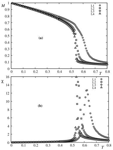
Figure 3: Magnetizations and susceptibilities of sublattices 1 and 3 first two cells vs temperature for $J_{s}=-1.0$ with $L=24$ and $D=0.1$. $L_{j}$ denotes the sublattice magnetization of layer $j$.

It is interesting to note that the surface layer has largest magnetization followed by that of the second layer, while the third and fourth layers have smaller magnetizations. This is not the case for non frustrated films where the surface magnetization is always smaller than the interior ones because of the effects of low-lying energy surface-localized magnon modes.diep79 ; diep81 One explanation can be advanced: due to the lack of neighbors surface spins suffer fluctuations due to the frustration less than the interior spins so they maintain their ordering up to a higher temperature. Let us decrease the $J_{s}$ strength. The surface spins then have smaller local field, so thermal fluctuations will reduce their ordering to a lower temperature. Figures 4 and 5 show respectively the cases where $J_{s}=-0.8$ and -0.5. Near $J_{s}=-0.8$ the crossover takes place: the surface magnetization becomes smaller than the interior ones for $J_{s}>-0.8$. Note that the magnetizations of second, third and fourth layers undergo a discontinuity at the transition temperature for $J_{s}=-0.8$ and -0.5. This suggests that the phase transitions for interior layers are of first order as it has been found for bulk FCC antiferromagnet.Diep1989fcc This should be checked in the future.

For weak $|J_{s}|$, there is only one transition for all layers. An example is shown in Fig. 6 for $J_{s}=-0.1$. Note that the first-order character disappears as there is no discontinuity of layer magnetizations at the transition temperature.

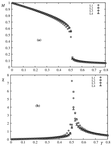
Figure 4: Magnetizations and susceptibilities of sublattices 1 and 3 of first two cells vs temperature for $J_{s}=-0.8$ with $L=24$ and $D=0.1$. $L_{j}$ denotes the sublattice magnetization of layer $j$.

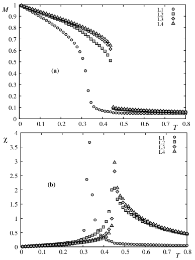
Figure 5: Magnetizations and susceptibilities of first two cells vs temperature for $J_{s}=-0.5$ with $L=24$ and $D=0.1$. $L_{j}$ denotes the sublattice magnetization of layer $j$. The susceptibility of sublattice 1 of the first cell is divided by a factor $5$ for presentation convenience.

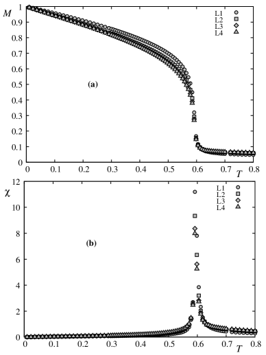
Figure 6: Magnetization and susceptibility of first two cells vs temperature for $J_{s}=-0.1$ with $L=24$ and $D=0.1$. $L_{j}$ denotes the sublattice magnetization of layer $j$.

In the region $-0.5<J_{s}<-0.45$, there is an interesting reentrant phenomenon. To facilitate the description of this phenomenon, let us show the phase diagram in the space ($J_{s},T_{c}$) in Fig. 7. In the region $-0.5<J_{s}<-0.45$, the GS is of type II as seen above. According to the phase diagram, we see that when the temperature increases from zero, the system goes through the phase of type II, undergoes a transition to enter the phase of type I before making a second transition to the paramagnetic phase at high temperature. This kind of behavior is termed as reentrant phenomenon which has been found by exact solutions in a number of very frustrated systems.diep91honeyc ; diep91Kago For a complete review on these exactly solved systems, the reader is referred to the chapter by Diep and GiacominiDiep-Giacomini in Ref. Diep2005, . We note here that the reentrance is often found near the frontier where two phases coexist in the GS.Diep2005 This is the case at $J_{s}=J_{s}^{c}=-0.5$.

The discontinued vertical line at $J_{s}=-0.5$ is a first-order line separating phases I and II. The coexistence of these two phases which do not have the same symmetry explains the first-order character of this line. To show it explicitly, we have calculated at $T=0.15$ the magnetization $M$ and the staggered magnetization $M_{st}$ of the first layer with varying $J_{s}$ across -O.5. From the GS configurations shown in Fig. 2, $M$ should be zero in phase I and finite in phase II, and vice-versa for $M_{st}$. This is observed at $T=0.15$ as shown in Fig. 8. The large discontinuity of $M$ and $M_{st}$ at $J_{s}=-0.5$ shows a very strong first-order character across the vertical line in Fig. 7.

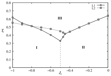
Figure 7: Critical temperature vs $J_{s}$ with $L=24$ and $D=0.1$. $L_{j}$ denotes data points for the sublattice magnetization of layer $j$. I and II denote ordering of type I and II defined in in Fig. 2. III is paramagnetic phase. The discontinued vertical line is a first-order line. See text for comments.

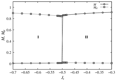
Figure 8: The magnetization $M$ and the staggered magnetization $M_{st}$ of first layer versus $J_{s}$ are shown, at $T=0.15$, with $L=24$ and $D=0.1$. I and II denote ordering of type I and II defined in Fig. 2. III is paramagnetic phase. See text for comments.

Let us discuss on finite-size effects in the transitions observed in Fig. 3 to Fig. 6. This is an important question because it is known that some apparent transitions are artifacts of small system sizes. To confirm the observed transitions, we have made a study of finite-size effects on the layer susceptibilities by using the accurate MC multi histogram technique.Ferrenberg1 ; Ferrenberg2 ; Ferrenberg3

At this point, let us recall that bulk Ising frustrated systems, unlike unfrustrated counterparts, have different transition natures: the antiferromagnetic FCC and HCP Ising lattices have strong first-order transition,Phani ; Polgreen ; Styer while the stacked antiferromagnetic triangular lattice has a controversial nature (see references in Ref. Plumer, ). The model studied here is the frustrated FCC film where surface effects can modify the strong first-order observed in its bulk counterpart.

Our results show that transitions at $J_{s}=-1$ and $J_{s}=-0.1$ are real second-order transitions obeying some scaling law. Figure 9 shows the size effects on the maximum of the susceptibilities of the first and second layers for $J_{s}=-0.1$, while Fig. 10 shows that of the third and fourth layers. As seen, the maximum of the susceptibilities $\chi^{\max}$ increases with increasing $L$.

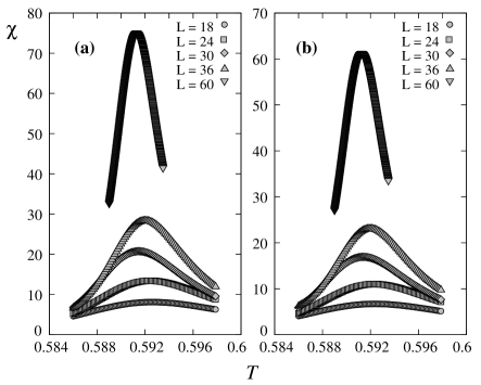
Figure 9: Susceptibilities of layer 1 (left) and 2 (right) are shown for various sizes $L$ as a function of temperature for $J_{s}=-0.1$ and $D=0.1$.

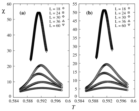
Figure 10: Susceptibilities of layer 3 (left) and 4 (right) are shown for various sizes $L$ as a function of temperature for $J_{s}=-0.1$ and $D=0.1$.

Using the scaling law $\chi^{\max}\propto L^{\gamma/\nu}$, we plot $\ln\chi^{\max}$ versus $\ln L$ in Fig. 11. The ratio of the critical exponents $\gamma/\nu$ is obtained by the slope of the straight line connecting the data points of each layer.

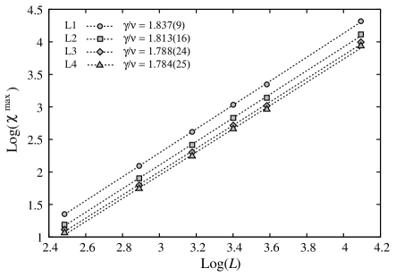
Figure 11: Maximum sublattice susceptibility $\chi^{\max}$ versus $L$ in the $\ln-\ln$ scale, for $J_{s}=-0.1$ and $D=0.1$. $L_{j}$ denotes the sublattice magnetization of layer $j$. The slopes of these lines give the ratios of exponents $\gamma/\nu$.

Within errors the third and fourth layers have the same value of $\gamma/\nu$ which is neither 2D nor 3D Ising universality classes, 1.75 and 2, respectively. The same for the the values of the first and second layers. The exponent $\nu$ can be obtained as follows. We calculate as a function of $T$ the magnetization derivative with respect to $\beta=(k_{B}T)^{-1}$: $V_{1}=\left<(\ln M)^{\prime}\right>=\left<E\right>-\left<ME\right>/\left<M\right>$ where $E$ is the system energy and $M$ the sublattice order parameter. We identify the maximum of $V_{1}$ for each size $L$. From the finite-size scaling we know that $V_{1}^{\max}$ is proportional to $L^{1/\nu}$.Ferrenberg3 We plot in Fig. 12 $\ln V_{1}^{\max}$ as a function of $\ln L$ for $J_{s}=-0.1$. The slope of each line gives $1/\nu$. For the case $J_{s}=-0.1$, we obtain $\nu=0.822\pm 0.020,0.795\pm 0.020,0.790\pm 0.020,0.782\pm 0.020$ for the first, second, third and fourth layers. These values are far from the 2D value ($\nu=1$). We deduce $\gamma=1.510\pm 0.010,1.442\pm 0.015,1.412\pm 0.025,1.395\pm 0.025$. The values of $\nu$ and $\gamma$ are decreased when one goes from the surface to the interior of the film.

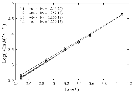
Figure 12: The maximum value of $\left<(\ln M)^{\prime}\right>=\left<E\right>-\left<ME\right>/\left<M\right>$ versus $L$ in the $\ln-\ln$ scale for $J_{s}=-0.1$, where $M$ is the sublattice order parameter. The slope of each line gives $1/\nu$. $L_{j}$ denotes the sublattice magnetization of layer $j$.

We show in Fig. 13 and Fig. 14 the maximum of sublattice magnetizations and their derivatives for the first two layers in the case of $J_{s}=-1$. We find $\nu_{1}=0.794\pm 0.022$, $\nu_{2}=0.834\pm 0.027$, $\gamma_{1}=1.524\pm 0.0.040$, and $\gamma_{2}=1.509\pm 0.022$.

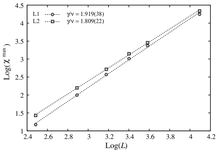
Figure 13: Maximum sublattice susceptibility $\chi^{\max}$ versus $L$ in the $\ln-\ln$ scale, for $J_{s}=-1$ and $D=0.1$. $L_{j}$ denotes the sublattice magnetization of layer $j$. The slopes of these lines give the ratios of exponents $\gamma/\nu$.

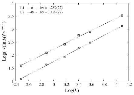
Figure 14: The maximum value of $\left<(\ln M)^{\prime}\right>=\left<E\right>-\left<ME\right>/\left<M\right>$ versus $L$ in the $\ln-\ln$ scale for $J_{s}=-1$, where $M$ is the sublattice order parameter. The slope of each line gives $1/\nu$. $L_{k}S_{j}$ denotes one sublattice magnetization of layer $j$.

Let us discuss on the values of the critical exponents obtained above. These values do not correspond neither to 2D nor 3D Ising models ($\gamma_{2D}=1.75$, $\nu_{2D}=1$, $\gamma_{3D}=1.241$, $\nu_{3D}=0.63$). There are multiple reasons for those deviations. Apart from numerical precisions and the modest sizes we used, there may be deep physical origins.

A first question which naturally arises is the effect of the frustration. The 3D version of this model, as said above, has a first-order transition, with a very strong character for the Ising casePhani ; Polgreen ; Styer and somewhat less strong for the continuous spin models.Diep1989fcc It has been shown that at finite temperature, the phenomenon called ”order by disorder” occurs leading to a reduction of degeneracy: only collinear configurations survive by an entropy effect.Diep1989fcc ; Villain ; Henley The infinite degeneracy is reduced to 6, i. e. the number of ways to put two AF spin pairs on a tetrahedron. The model is equivalent to 6-state Potts model. The first-order transition observed in the 3D case is in agreement with the Potts criterion according to which the transition in $q$-state Potts model is of first-order in 3D for $q\geq 3$.

In the case of a film with finite thickness studied here, it appears that the first-order character is lost.

A first possible cause is from the degeneracy. According to the results shown in the previous section, the GS degeneracy is 2 or 4 depending to $J_{s}$. If we compare to the Potts criterion according to which the transition is of first-order in 2D only when $q>4$, then the transition in thin films should be of second order. That is indeed what we observed.

Another possible cause for the second-order transition observed here is from the role of the correlation in the film. For second-order transitions, some arguments, such as those from renormalization group, say that the correlation length in the direction perpendicular to the film is finite, hence it is irrelevant to the criticality, the film should have the 2D character. If a transition is of first order in 3D, i. e. the correlation length is finite at the transition temperature, then in thin films the thickness effect may be important: if the thickness is larger than the correlation length at the transition, than the first-order transition should remain. On the other hand, if the thickness is smaller than that correlation length, the spins then feel an ”infinite” correlation length across the film thickness. As a consequence, two pictures can be thought of: i) the whole system may be correlated and the first-order character is to become a second-order one ii) the correlation length is longer but still finite, the transition remains of first order.

At this point, we would like to emphasize that, in the case of simple surface conditions, i.e. no significant deviation of the surface parameters with respect to those of the bulk, the bulk behavior is observed when the thickness becomes larger than a few dozens of atomic layers:diep79 ; diep81 surface effects are insignificant on some thermodynamic properties such as the value of the critical temperature, the mean value of magnetization at a given $T$, … It should be however stressed that the criticality is very different. It depends on the correlation length compared to the thickness: for example, we have obtained in the case of simple cubic films with Ising model the critical exponents identical to those of 2D Ising universality class up to thickness of 9 layers.tu Due to the small thickness used here, we think that the 2D character should be assumed.

Now for the anisotropy, remember that in the case studied here, we do not deal with the discrete Ising model but rather an Ising-like Heisenberg model. The deviation from the 2D values may then result in part from a complex coupling between the Ising-like symmetry and the continuous nature of the classical Heisenberg spins. This deviation may be important if the anisotropy constant $D$ is small as in the case studied here.

To conclude this paragraph, we believe, from physical arguments given above, that the critical exponents obtained above which do not belong to any known universality class may result from different physical mechanisms. This is a subject of future investigations.

IV Green’s Function Method

We can rewrite the full Hamiltonian (1) in the local framework as

$$\mathcal{H} = -\sum_{<i,j>}J_{i,j}\Bigg{\{}\frac{1}{4}\left(\cos\theta_{ij}-1\right)\left(S^{+}_{i}S^{+}_{j}+S^{-}_{i}S^{-}_{j}\right)$$ (8)

$$+ \frac{1}{4}\left(\cos\theta_{ij}+1\right)\left(S^{+}_{i}S^{-}_{j}+S^{-}_{i}S^{+}_{j}\right)$$

$$+ \frac{1}{2}\sin\theta_{ij}\left(S^{+}_{i}+S^{-}_{i}\right)S^{z}_{j}-\frac{1}{2}\sin\theta_{ij}S^{z}_{i}\left(S^{+}_{j}+S^{-}_{j}\right)$$

$$+ \cos\theta_{ij}S^{z}_{i}S^{z}_{j}\Bigg{\}}-\sum_{<i>}I_{i}(S^{z}_{i})^{2}$$

where $\cos\left(\theta_{ij}\right)$ is the angle between two NN spins.

To study properties of quantum spins over a large region of temperatures, there are only a few methods which give relatively correct results. Among them, the GF method is known to recover the exact results at very low-$T$ obtained from the spin-wave theory. In addition, it is better than the spin-wave theory at higher temperatures and can be used up to the transition temperature with of course less precision on the nature of the phase transition. It should be emphasized that the GF method is much better than other methods such as mean-field theories in estimating the value of the critical temperature. We choose here this method to study quantum effects at low $T$ and to obtain the phase diagram at high $T$.

The GF method can be used for non collinear spin configurations.Rocco In the case studied here, one has a collinear one because of the Ising-like anisotropy. In this case, we define two double-time GF bytahir

$$G_{ij}(t,t^{\prime}) = \ll S^{+}_{i}(t);S^{-}_{j}(t^{\prime})\gg,$$ (9)

$$F_{ij}(t,t^{\prime}) = \ll S^{-}_{i}(t);S^{+}_{j}(t^{\prime})\gg.$$ (10)

The equations of motion for $G_{ij}(t,t^{\prime})$ and $F_{ij}(t,t^{\prime})$ are written by

$$i\frac{d}{dt}G_{i,j}\left(t,t^{\prime}\right) = \left<\left[S^{+}_{i}\left(t\right),S^{-}_{j}\left(t^{\prime}\right)\right]\right>\delta\left(t-t^{\prime}\right)$$ (11)

$$- \left<\left<\left[\mathcal{H},S^{+}_{i}\left(t\right)\right];S^{-}_{j}\left(t^{\prime}\right)\right>\right>,$$

$$i\frac{d}{dt}F_{i,j}\left(t,t^{\prime}\right) = \left<\left[S^{-}_{i}\left(t\right),S^{-}_{j}\left(t^{\prime}\right)\right]\right>\delta\left(t-t^{\prime}\right)$$ (12)

$$- \left<\left<\left[\mathcal{H},S^{-}_{i}\left(t\right)\right];S^{-}_{j}\left(t^{\prime}\right)\right>\right>,$$

We shall neglect higher-order correlations by using the Tyablikov decoupling schemeTyablikov which is known to be valid for exchange terms.fro Then, we introduce the following Fourier transforms

$$G_{i,j}\left(t,t^{\prime}\right) = \frac{1}{\Delta}\int\int d\mathbf{k}_{xy}\frac{1}{2\pi}\int^{+\infty}_{-\infty}d\omega e^{-i\omega\left(t-t^{\prime}\right)}.$$ (13)

$$\hskip 19.91684ptg_{n,n^{\prime}}\left(\omega,\mathbf{k}_{xy}\right)e^{i\mathbf{k}_{xy}\cdot\left(\mathbf{R}_{i}-\mathbf{R}_{j}\right)},$$

$$F_{i,j}\left(t,t^{\prime}\right) = \frac{1}{\Delta}\int\int d\mathbf{k}_{xy}\frac{1}{2\pi}\int^{+\infty}_{-\infty}d\omega e^{-i\omega\left(t-t^{\prime}\right)}.$$ (14)

$$\hskip 19.91684ptf_{n,n^{\prime}}\left(\omega,\mathbf{k}_{xy}\right)e^{i\mathbf{k}_{xy}\cdot\left(\mathbf{R}_{i}-\mathbf{R}_{j}\right)},$$

where $\omega$ is the spin-wave frequency, $\mathbf{k}_{xy}$ denotes the wave-vector parallel to $xy$ planes, $\mathbf{R}_{i}$ is the position of the spin at the site $i$, $n$ and $n^{\prime}$ are respectively the indices of the layers where the sites $i$ and $j$ belong to. The integral over $\mathbf{k}_{xy}$ is performed in the first Brillouin zone whose surface is $\Delta$ in the $xy$ reciprocal plane.

The Fourier transforms of the retarded GF satisfy a set of equations rewritten under the following matrix form

$$\mathbf{M}\left(\omega\right)\mathbf{g}=\mathbf{u},$$ (15)

where $\mathbf{M}\left(\omega\right)$ is a square matrix $\left(2N_{z}\times 2N_{z}\right)$, $\mathbf{g}$ and $\mathbf{u}$ are the column matrices which are defined as follows

$$\mathbf{g}=\left(\begin{array}[]{c}g_{1,n^{\prime}}\\ f_{1,n^{\prime}}\\ \vdots\\ g_{N_{z},n^{\prime}}\\ f_{N_{z},n^{\prime}}\\ \end{array}\right),\mathbf{u}=\left(\begin{array}[]{c}2\left<S^{z}_{1}\right>\delta_{1,n^{\prime}}\\ 0\\ \vdots\\ 2\left<S^{z}_{N_{z}}\right>\delta_{N_{z},n^{\prime}}\\ 0\\ \end{array}\right),$$ (16)

and

$$\mathbf{M}\left(\omega\right)=\left(\begin{array}[]{ccccc}A^{+}_{1}&B_{1}&D^{+}_{1}&D^{-}_{1}&\cdots\\ -B_{1}&A^{-}_{1}&-D^{-}_{1}&-D^{+}_{1}&\vdots\\ \vdots&\cdots&\cdots&\cdots&\vdots\\ \vdots&C^{+}_{N_{z}}&C^{-}_{N_{z}}&A^{+}_{N_{z}}&B_{N_{z}}\\ \cdots&-C^{-}_{N_{z}}&-C^{+}_{N_{z}}&-B_{N_{z}}&A^{-}_{N_{z}}\\ \end{array}\right),$$ (17)

where

$$A_{n}^{\pm} = \omega\pm\Big{[}\frac{1}{2}J_{n}\left<S^{z}_{n}\right>\left(Z\gamma\right)\left(\cos\theta_{n}+1\right)$$ (18)

$$- J_{n}\left<S^{z}_{n}\right>Z\cos\theta_{n}-2I_{n}\left<S^{z}_{n}\right>$$

$$- 2J_{n,n+1}\left<S^{z}_{n+1}\right>\cos\theta_{n,n+1}^{(a)}$$

$$- 2J_{n,n+1}\left<S^{z}_{n+1}\right>\cos\theta_{n,n+1}^{(b)}$$

$$- 2J_{n,n-1}\left<S^{z}_{n-1}\right>\cos\theta_{n,n-1}^{(a)}$$

$$- 2J_{n,n-1}\left<S^{z}_{n-1}\right>\cos\theta_{n,n-1}^{(b)}\Big{]},$$

$$B_{n} = \frac{1}{2}J_{n}\left<S^{z}_{n}\right>\left(Z\gamma\right)\left(\cos\theta_{n}-1\right),$$ (19)

$$C_{n}^{\pm} = J_{n,n-1}\left<S^{z}_{n}\right>\left(\cos\theta_{n,n-1}^{(a)}\pm 1\right)$$ (20)

$$+ J_{n,n-1}\left<S^{z}_{n}\right>\left(\cos\theta_{n,n-1}^{(b)}\pm 1\right),$$

$$D_{n}^{\pm} = J_{n,n+1}\left<S^{z}_{n}\right>\left(\cos\theta_{n,n+1}^{(a)}\pm 1\right)$$ (21)

$$+ J_{n,n+1}\left<S^{z}_{n}\right>\left(\cos\theta_{n,n+1}^{(b)}\pm 1\right),$$

in which, $Z=4$ is the number of in-plane NN, $\theta_{n,n\pm 1}^{(a)}$ the angle between two NN spins of sublattice 1 and 3 belonging to the layers $n$ and $n\pm 1$ (see Fig. 2), $\theta_{n,n\pm 1}^{(b)}$ the angle between two NN spins of sublattice 1 and 4, $\theta_{n}$ the angle between two in-plane NN spins in the layer $n$, and

$$\gamma=\frac{1}{Z}\left[4\cos\left(\frac{k_{x}a}{2}\right)\cos\left(\frac{k_{y}a}{2}\right)\right].$$

Here, for compactness we have used the following notations:

i) $J_{n}$ and $D_{n}$ are the in-plane interactions. In the present model $J_{n}$ is equal to $J_{s}$ for the two surface layers and equal to $J$ for the interior layers. All $D_{n}$ are set to be $D$.

ii) $J_{n,n\pm 1}$ are the interactions between a spin in the $n$-th layer and its neighbor in the $(n\pm 1)$-th layer. Of course, $J_{n,n-1}=0$ if $n=1$, $J_{n,n+1}=0$ if $n=N_{z}$.

Solving det$|\mathbf{M}|=0$, we obtain the spin-wave spectrum $\omega$ of the present system. The solution for the GF $g_{n,n}$ is given by

$$g_{n,n}=\frac{\left|\mathbf{M}\right|_{n}}{\left|\mathbf{M}\right|},$$ (22)

with $\left|\mathbf{M}\right|_{n}$ is the determinant made by replacing the $n$-th column of $\left|\mathbf{M}\right|$ by $\mathbf{u}$ in (16). Writing now

$$\left|\mathbf{M}\right|=\prod_{i}\left(\omega-\omega_{i}\left(\mathbf{k}_{xy}\right)\right),$$ (23)

one sees that $\omega_{i}\left(\mathbf{k}_{xy}\right),\ i=1,\cdots,\ N_{z}$, are poles of the GF $g_{n,n}$. $\omega_{i}\left(\mathbf{k}_{xy}\right)$ can be obtained by solving $\left|\mathbf{M}\right|=0$. In this case, $g_{n,n}$ can be expressed as

$$g_{n,n}=\sum_{i}\frac{f_{n}\left(\omega_{i}\left(\mathbf{k}_{xy}\right)\right)}{\left(\omega-\omega_{i}\left(\mathbf{k}_{xy}\right)\right)},$$ (24)

where $f_{n}\left(\omega_{i}\left(\mathbf{k}_{xy}\right)\right)$ is

$$f_{n}\left(\omega_{i}\left(\mathbf{k}_{xy}\right)\right)=\frac{\left|\mathbf{M}\right|_{n}\left(\omega_{i}\left(\mathbf{k}_{xy}\right)\right)}{\prod_{j\neq i}\left(\omega_{j}\left(\mathbf{k}_{xy}\right)-\omega_{i}\left(\mathbf{k}_{xy}\right)\right)}.$$ (25)

Next, using the spectral theorem which relates the correlation function $\langle S^{-}_{i}S^{+}_{j}\rangle$ to the GF,zu one has

$$\left<S^{-}_{i}S^{+}_{j}\right> = \lim_{\varepsilon\rightarrow 0}\frac{1}{\Delta}\int\int d\mathbf{k}_{xy}\int^{+\infty}_{-\infty}\frac{i}{2\pi}\big{(}g_{n,n^{\prime}}\left(\omega+i\varepsilon\right)$$ (26)

$$- g_{n,n^{\prime}}\left(\omega-i\varepsilon\right)\big{)}\cdot\frac{d\omega}{e^{\beta\omega}-1}e^{i\mathbf{k}_{xy}\cdot\left(\mathbf{R}_{i}-\mathbf{R}_{j}\right)},$$

where $\epsilon$ is an infinitesimal positive constant and $\beta=1/k_{B}T$, $k_{B}$ being the Boltzmann constant.

Using the GF presented above, we can calculate self-consistently various physical quantities as functions of temperature $T$. We start the self-consistent calculation from $T=0$ with a small step for temperature: $5\times 10^{-3}$ at low $T$ and $10^{-1}$ near $T_{c}$ (in units of $J/k_{B}$). The convergence precision has been fixed at the fourth figure of the values obtained for the layer magnetizations. We know from the previous section that the spin configuration is collinear, therefore in this section, we shall use a large value of Ising anisotropy $D$ in order to get a rapid numerical convergence. For numerical calculation, we will use $D=4$ and $J=-1$ and a size of $80^{2}$ points in the first Brillouin zone.

Figure 15 shows the sublattice magnetizations of the first four layers. As seen, the first-layer one is larger than the other three just as in the case of the classical spins shown in Fig. 3. This difference in sublattice magnetization between layers vanishes at $J_{s}\simeq-0.8$ as seen in Fig. 16. Again here, one has a good agreement with the case of classical spins shown in Fig. 4.

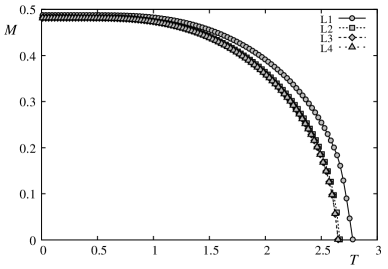
Figure 15: Layer magnetization of first four layers vs temperature for $J_{s}=-1.0$ and $D=4$. $L_{j}$ denotes the sublattice magnetization of layer $j$. Note that except the first layer, all other layer magnetizations coincide in this figure scale.

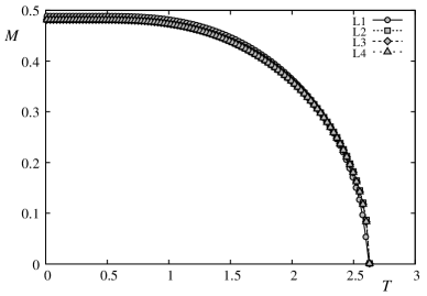
Figure 16: Layer magnetizations of first four layers vs temperature for $J_{s}=-0.8$ and $D=4$. $L_{j}$ denotes the sublattice magnetization of layer $j$. Note that all layer magnetizations coincide in this figure scale.

For $J_{s}>-0.8$, the sublattice magnetization of the first layer is larger at low $T$ and higher at high $T$ as seen in Fig. 17 for $J_{s}=-0.5$. This crossover of sublattice magnetizations comes from the competition between quantum fluctuations and the strength of $J_{s}$: when $|J_{s}|$ is small, quantum fluctuations of the surface layer are small yielding a small zero-point spin contraction for surface spins at $T=0$. So, surface magnetization is higher than the interior ones. At higher $T$, however, small $|J_{s}|$ gives rise to a small local field for surface spins which in turn yields a smaller surface magnetization at high $T$. This crossover has been found earlier in antiferromagnetic superlattices and films.Diep1989sl ; diep91-af-films

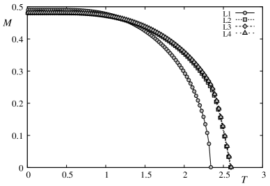
Figure 17: Layer magnetization of first four layers vs temperature for $J_{s}=-0.5$ and $D=4$. $L_{j}$ denotes the sublattice magnetization of layer $j$. Note that except the first layer, all other layer magnetizations coincide in this figure scale. See text for comments on the crossover of surface magnetization.

For $J_{s}=-0.1$, there is no more crossover at low $T$ as seen in Fig. 18. Moreover, there is only a single transition at $T_{c}\simeq 2.65$ for both surface and interior layers.

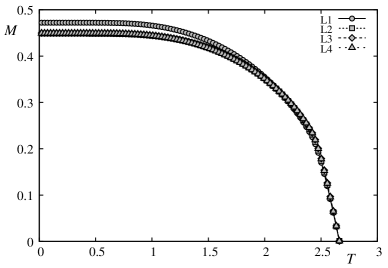
Figure 18: Layer magnetization of first four layers vs temperature for $J_{s}=-0.1$ and $D=4$. $L_{j}$ denotes the sublattice magnetization of layer $j$. Only at low $T$ the surface magnetization is distinct from the other ones.

We summarize in Fig. 19 the phase diagram for the quantum spin case obtained with the GF method. The vertical discontinued line indicates the boundary between ordered phases of types I and II. Phase III is paramagnetic. Note the following interesting points:

i) for $J_{s}<-0.4$ there is a surface transition distinct from that of interior layers,

ii) for $J_{s}<-0.8$, surface transition occurs at a temperature higher than that of interior layers,

iii) there is a reentrance between $J_{s}=-0.4$ and $J_{s}=-0.5$. This is very similar to the phase diagram of the classical spins obtained by MC simulations shown in Fig. 7.

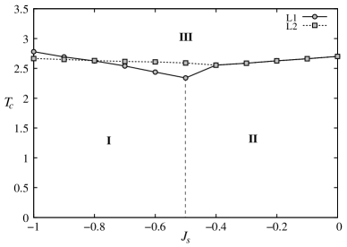
Figure 19: Phase diagram obtained by the Green’s function method with $D=4$. $L_{j}$ denotes the transition temperature of the sublattice magnetization of layer $j$. See text for comments.

V Concluding Remarks

We have studied in this paper the properties of a thin film made from a fully frustrated material, namely the FCC antiferromagnet. We have considered both classical and quantum Heisenberg spin model with an Ising-like single-ion anisotropy. The classical case was treated by Monte Carlo simulation while the quantum case was studied by the Green’s function method. Several important results are found in this paper. We found that the presence of a surface reduces the GS degeneracy of the fully-frustrated FCC antiferromagnet and there exists a critical value of the in-plane surface interaction $J_{s}^{c}=-0.5$ which separates the GS configuration of type I from that of type II. We have studied the phase transition of the system. The surface spin ordering is destroyed in general at a temperature different from that of the interior layers. We found that in a small region just above $J_{s}^{c}$ there is a reentrant phase: with decreasing $T$ the system first changes from the paramagnetic phase to the type II phase, and then enters at a lower temperature into the type I phase. The critical behaviors of surface and interior layers have been shown and discussed.

We hope that these unusual surface properties will help experimentalists to analyze their data obtained for real systems where frustration plays an important role.

One of us (VTN) thanks the ”Asia Pacific Center for Theoretical Physics” (South Korea) for a financial post-doc support and hospitality during the period 2005-2006 where part of this work was carried out.

References

- (1) See reviews on theories and experiments given in Frustrated Spin Systems, ed. H. T. Diep, World Scientific (2005).
- (2) A. Zangwill, Physics at Surfaces, Cambridge University Press (1988).
- (3) Ultrathin Magnetic Structures, vol. I and II, J.A.C. Bland and B. Heinrich (editors), Springer-Verlag (1994).
- (4) K. Binder, in Phase Transitions and Critical Phenomena, ed. by C. Domb, J.L. Lebowitz (Academic, London, 1983) vol. 8.
- (5) H.W. Diehl, in Phase Transitions and Critical Phenomena, ed. by C. Domb, J.L. Lebowitz (Academic, London, 1986) vol. 10, H.W. Diehl, Int. J. Mod. Phys. B 11, 3503 (1997).
- (6) M. N. Baibich, J. M. Broto, A. Fert, F. Nguyen Van Dau, F. Petroff, P. Etienne, G. Creuzet, A. Friederich and J. Chazelas, Phys. Rev. Lett. 61, 2472 (1988).
- (7) P. Grunberg, R. Schreiber, Y. Pang, M. B. Brodsky and H. Sowers, Phys. Rev. Lett. 57, 2442 (1986); G. Binash, P. grunberg, F. Saurenbach and W. Zinn, Phys. Rev. B 39, 4828 (1989).
- (8) A. Barth l my et al, J. Mag. Mag. Mater. 242-245, 68 (2002).
- (9) See review by E. Y. Tsymbal and D. G. Pettifor, Solid State Physics (Academic Press, San Diego), Vol. 56, pp. 113-237 (2001).
- (10) See V. Thanh Ngo, H. Viet Nguyen, H. T. Diep and V. Lien Nguyen, Phys. Rev. B. 69, 134429 (2004) and references on magnetic multilayers cited therein.
- (11) See V. Thanh Ngo and H. T. Diep, Phys. Rev. B. 75, 035412 (2007) and references on surface effects cited therein.
- (12) T. A. Kaplan and N. Menyuk, Phil. Mag. , in press (private communication), and references therein.
- (13) T. Oguchi, H. Nishimori and Y. Taguchi, J. Phys. Soc. Jpn 54, 4494 (1985).
- (14) P. Lallemand, H. T. Diep, A. Ghazali and G. Toulouse, J. Phys. (Paris) Lett. 46, L1087 (1985).
- (15) H. T. Diep and H. Kawamura, Phys. Rev. B 40, 7019 (1989).
- (16) J. L. Lebowitz and M. H. Kalos, Phys. Rev. B 21, 4027 (1980).
- (17) T. L. Polgreen, Phys. Rev. B 29, 1468 (1984).
- (18) D. F. Styer, Phys. Rev. B 32, 393 (1985).
- (19) H. T. Diep, Phys. Rev. B 45, 2863 (1992), and references therein.
- (20) N. D. Mermin and H. Wagner, Phys. Rev. Lett. 17, 1133 (1966).
- (21) H. T. Diep, J.C. S. Levy and O. Nagai, Phys. Stat. Solidi (b) 93, 351 (1979).
- (22) H. T. Diep, Phys. Stat. Solidi (b) , 103, 809 (1981).
- (23) H. T. Diep, M. Debauche and H. Giacomini, Phys. Rev. B (rapid communication) 43, 8759 (1991).
- (24) M. Debauche, H. T. Diep, H. Giacomini and P. Azaria, Phys. Rev. B 44, 2369 (1991).
- (25) H. T. Diep and H. Giacomini, see chapter Frustration - Exactly Solved Frustrated Models in Ref. Diep2005, .
- (26) A. M. Ferrenberg and R. H. Swendsen, Phys. Rev. Let. 61, 2635 (1988).
- (27) A. M. Ferrenberg and R. H. Swendsen, Phys. Rev. Let. 63, 1195 (1989).
- (28) A. M. Ferrenberg and D. P. Landau, Phys. Rev. B 44, 5081 (1991).
- (29) J. Villain, R. Bideaux, J.P. Carton and R. Conte, J. Phys. (Paris) 41, 1263 (1980).
- (30) C. Henley, J. Appl. Phys. 61, 3962 (1987); Phys. Rev. Lett. 62, 2056 (1989).
- (31) M. L. Plumer, A. Mailhot, R. Ducharme, A. Caill and H. T. Diep, Phys. Rev. B 47, 14312 (1993).
- (32) X. T. Tu, V. T. Ngo and H. T. Diep, unpublished (2007).
- (33) See for example R. Quartu and H.T. Diep, Phys. Rev. B 55, 2975 (1997); C. Santamaria, R. Quartu and H. T. Diep, J. Appl. Physics 84, 1953 (1998).
- (34) R. A. Tahir-Kheli and D. Ter Haar, Phys. Rev. 127, 88 (1962).
- (35) N. N. Bogolyubov and S. V. Tyablikov, Doklady Akad. Nauk S.S.S.R. 126, 53 (1959) [translation: Soviet Phys.-Doklady 4 604 (1959)].
- (36) P. Fröbrich, P. J. Jensen and P. J. Kuntz, Eur. Phys. J B 13, 477 (2000) and references therein.
- (37) D. N. Zubarev, Usp. Fiz. Nauk 187, 71 (1960)[translation: Soviet Phys.-Uspekhi 3 320 (1960)].
- (38) H. T. Diep, Phys. Rev. B 40, 4818 (1989).
- (39) H. T. Diep, Phys. Rev. B 43, 8509 (1991).