Multiple Antenna Secure Broadcast over Wireless Networks

Abstract

In wireless data networks, communication is particularly susceptible to eavesdropping due to its broadcast nature. Security and privacy systems have become critical for wireless providers and enterprise networks. This paper considers the problem of secret communication over the Gaussian broadcast channel, where a multi-antenna transmitter sends independent confidential messages to two users with perfect secrecy. That is, each user would like to obtain its own message reliably and confidentially. First, a computable Sato-type outer bound on the secrecy capacity region is provided for a multi-antenna broadcast channel with confidential messages. Next, a dirty-paper secure coding scheme and its simplified version are described. For each case, the corresponding achievable rate region is derived under the perfect secrecy requirement. Finally, two numerical examples demonstrate that the Sato-type outer bound is consistent with the boundary of the simplified dirty-paper coding secrecy rate region.

1 Introduction

The need for efficient, reliable, and secure data communication over wireless networks has been rising rapidly for decades. Due to its broadcast nature, wireless communication is particularly susceptible to eavesdropping. The inherent problematic nature of wireless networks exposes not only the risks and vulnerabilities that a malicious user can exploit and severely compromise the network but also multiplies information confidentiality concerns with respect to in-network terminals. Hence, security and privacy systems have become critical for wireless providers and enterprise networks.

In this work, we consider multiple antenna secure broadcast in wireless networks. This research is inspired by the seminal paper [1], in which Wyner introduced the so-called wiretap channel and proposed an information theoretic approach to secure communication schemes. Under the assumption that the channel to the eavesdropper is a degraded version of that to the desired receiver, Wyner characterized the capacity-secrecy tradeoff for the discrete memoryless wiretap channel and showed that secure communication is possible without sharing a secret key. Later, the result was extended by Csiszár and Körner who determined the secrecy capacity for the non-degraded broadcast channel (BC) with a single confidential message set intended for one of the users [2].

In more general wireless network scenarios, secure communication may involve multiple users and multiple antennas. Motivated by wireless communications, where transmitted signals are broadcast and can be received by all users within the communication range, a significant research effort has been invested in the study of the information-theoretic limits of secure communication in different wireless network environments [3, 4, 5, 6, 7, 8, 9, 10].

This issues motivate us to study the multi-antenna Gaussian broadcast channel with confidential messages (MGBC-CM), in which independent confidential messages from a multi-antenna transmitter are to be communicated to two users. The corresponding broadcast communication model is shown in Fig. 1. Each user would like to obtain its own message reliably and confidentially.

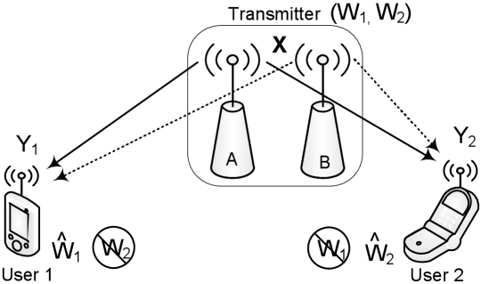
Figure 1: Multiple-antenna Gaussian broadcast channel with confidential message

To give insight into this problem, we first consider a single antenna Gaussian broadcast channel (GBC). Note that this channel is degraded [11], which means that if a message can be successfully decoded by the inferior user, then the superior user is also ensured of decoding it. Hence, the secrecy rate of the inferior user is zero and this problem is reduced to the scalar Gaussian wiretap channel problem [12] whose secrecy capacity is now the maximum rate achievable by the superior user. This analysis gives rise to the question: can the transmitter, in fact, communicate with both users confidentially at nonzero rate under some other conditions? Roughly speaking, the answer is in the affirmative. In particular, the transmitter can communicate when equipped with sufficiently separated multiple antennas.

We here have two goals motivated directly by questions arising in practice. The first is to determine the condition under which both users can obtain their own messages reliably and confidentially. This is equivalent to evaluating the secrecy capacity region for the MGBC-CM. The second is to show how the transmitter should broadcast securely, which is equivalent to designing an achievable secure coding scheme. To this end, a computable Sato-type outer bound on the secrecy capacity region is developed for the MGBC-CM in Sec. 3. Next, a dirty-paper secure coding scheme and its simplified version are described. For each case, the corresponding achievable rate region is derived under perfect secrecy requirement in Sec. 4. Finally, two numerical examples demonstrate that the Sato-type outer bound is consistent with the boundary of the simplified dirty-paper coding (DPC) secrecy rate region in Sec. 5.

2 System Model

We consider the communication of confidential messages to two users over a Gaussian broadcast channel via $t$ transmit-antennas. Each user is equipped with a single receive-antenna. The received signals at user 1 and user 2 are are modeled as

$$y_{1,i} =\mathbf{h}^{H}\mathbf{x}_{i}+z_{1,i}$$

$$y_{2,i} =\mathbf{g}^{H}\mathbf{x}_{i}+z_{2,i},\qquad i=1,\ldots,n$$ (1)

where $\mathbf{x}_{i}\in\mathbb{C}^{t}$ is the transmitted vector at time $i$, $z_{1,i}$ and $z_{2,i}$ correspond to two independent, zero-mean, unit-variance, complex Gaussian noise sequences, and $\mathbf{h},\,\mathbf{g}\in\mathbb{C}^{t}$ are channel attenuation vectors corresponding to user 1 and user 2, respectively. The channel input is constrained by

$$\frac{1}{n}\sum_{i=1}^{n}|\mathbf{x}_{i}|^{2}\leq A$$ (2)

where $A$ is the total transmit energy per channel use. We also assume that both the transmitter and receivers are aware of the attenuation vectors $\mathbf{h}$ and $\mathbf{g}$.

As shown in Fig. 1, the transmitter intends to send an independent confidential message $W_{k}\in\{1,\dots,M_{k}\}\triangleq{\mathcal{W}}_{k}$ to the respective user $k\in\{1,\,2\}$ in $n$ channel uses. To increase the randomness of transmitted messages, we consider a stochastic encoder at the transmitter. More explicitly, the encoder is specified by a matrix of conditional probability density $f(\mathbf{x}^{n}|w_{1},w_{2})$, where $\mathbf{x}^{n}=[\mathbf{x}_{1},\ldots,\mathbf{x}_{n}]$ and $w_{k}\in{\mathcal{W}}_{k}$. In other words, $f(\mathbf{x}^{n}|w_{1},w_{2})$ is the probability density associated with the conditional probability that the messages $(w_{1},w_{2})$ are encoded as the channel input $\mathbf{x}^{n}$.

The decoding function at user $k$ is a mapping $\phi_{k}\,:\,\mathbb{C}^{n}\rightarrow{\mathcal{W}}_{k}$. The secrecy levels with respect to the confidential messages $W_{1}$ and $W_{2}$ are measured, respectively, at receivers $1$ and $2$ with respect to the normalized equivocations

$$\frac{1}{n}H(W_{2}|Y_{1}^{n},W_{1})\quad\text{and}\quad\frac{1}{n}H(W_{1}|Y_{2}^{n},W_{2}).$$ (3)

An $(M_{1},M_{2},n,P_{e})$ code for the broadcast channel consists of the encoding function $f$, decoding functions $\phi_{1}$, $\phi_{2}$, and the maximum error probability $P_{e}\triangleq\max\{P_{e,1},\,P_{e,2}\}$, where $P_{e,k}$ is the error probability for user $k$ given by

$$P_{e,k} =P\bigl{[}\phi_{k}(Y_{k}^{n})\neq w_{k}\bigr{]}.$$ (4)

A rate pair $(R_{1},\,R_{2})$ is said to be achievable for the broadcast channel with confidential messages if, for any $\epsilon>0$, there exists an $(M_{1},M_{2},n,P_{e})$ code that satisfies $P_{e}\leq\epsilon$, $M_{k}\geq 2^{nR_{k}}$, for $k=1,2$, and the perfect secrecy requirement

$$H(W_{1})-H(W_{1}|Y_{2}^{n},W_{2}) \leq n\epsilon\quad\text{and}\quad H(W_{2})-H(W_{2}|Y_{1}^{n},W_{1})\leq n\epsilon.$$ (5)

The secrecy capacity region of ${\mathcal{C}}_{\rm BCC}$ of the MGBC-CM is the closure of the set of all achievable rate pairs $(R_{1},\,R_{2})$.

3 Outer Bound on the Secrecy Capacity Region

3.1 Sato-Type Outer Bound

We first consider a Sato-type bound that can be applied to both discrete memoryless and Gaussian broadcast channels with confidential messages (BC-CM). Let ${\mathcal{P}}$ be the set of channels $P_{\widetilde{Y}_{1},\widetilde{Y}_{2}|\mathbf{X}}$ that have the same marginal distributions as $P_{Y_{1},Y_{2}|\mathbf{X}}$, i.e.,

$$P_{\widetilde{Y}_{1}|\mathbf{X}}(y_{1}|\mathbf{x})=P(y_{1}|\mathbf{x})\quad\text{and}\quad P_{\widetilde{Y}_{2}|\mathbf{X}}(y_{2}|\mathbf{x})=P(y_{2}|\mathbf{x})$$ (6)

for all $y_{1}$, $y_{2}$ and $\mathbf{x}$. Let ${\mathcal{R}}_{\rm O}\bigl{(}P_{\widetilde{Y}_{1},\widetilde{Y}_{2}|\mathbf{X}},\,P_{\mathbf{X}}\bigr{)}$ denote the union of all rate pairs $(R_{1},\,R_{2})$ satisfying

$$R_{1} \leq I(\mathbf{X};\widetilde{Y}_{1}|\widetilde{Y}_{2})\quad\text{and}\quad R_{2}\leq I(\mathbf{X};\widetilde{Y}_{2}|\widetilde{Y}_{1})$$ (7)

for given distributions $P_{\mathbf{X}}$ and $P_{\widetilde{Y}_{1},\widetilde{Y}_{2}|\mathbf{X}}$.

Theorem 3.1

The secrecy capacity region ${\mathcal{C}}_{\rm BCC}$ of the BC-CM satisfies

$${\mathcal{C}}_{\rm BCC}\subseteq\bigcap_{P_{\widetilde{Y}_{1},\widetilde{Y}_{2}|\mathbf{X}}\in{\mathcal{P}}}\left\{\bigcup_{P_{\mathbf{X}}}{\mathcal{R}}_{\rm O}\bigl{(}P_{\widetilde{Y}_{1},\widetilde{Y}_{2}|\mathbf{X}},\,P_{\mathbf{X}}\bigr{)}\right\}.$$ (8)

Proof

See the Appendix.

Remark 1

The outer bound (8) follows by letting the users decode the message in a cooperative manner, while evaluating the secrecy level in an individual manner. Hence, the eavesdropped signal is always a degraded version of the entire received signal. This permits the use of the wiretap channel result of [1].

Remark 2

Although Theorem 3.1 is based on a degraded argument, the outer bound (8) can be applied to general broadcast channels with confidential messages.

3.2 Sato-Type Outer Bound for the Gaussian BC-CM

For the Gaussian channel case, we can simplify the outer bound (8) using the following steps. First, the channel family ${\mathcal{P}}$ is the set of channels (1) where $z_{1}$ and $z_{2}$ are replaced by arbitrarily correlated, zero-mean, unit-variance, Gaussian random variables $\widetilde{z}_{1}$ and $\widetilde{z}_{2}$ with covariance $\nu$. Furthermore, we consider a new coordinate transform as the setting of [10] and rewrite the broadcast channel model (1) as follows:

$$y_{1} =|\mathbf{h}|s_{1}+\widetilde{z}_{1}$$

$$y_{2} =\alpha|\mathbf{g}|s_{1}+\sqrt{1-|\alpha|^{2}}|\mathbf{g}|s_{2}+\widetilde{z}_{2}.$$ (9)

where

$$\alpha =\frac{\mathbf{g}^{H}\mathbf{h}}{|\mathbf{h}||\mathbf{g}|},\quad s_{1}=\frac{\mathbf{h}^{H}\mathbf{x}}{|\mathbf{h}|}\quad\text{and}~{}s_{2}=\frac{(|\mathbf{h}|\mathbf{g}-\alpha|\mathbf{g}|\mathbf{h})^{H}\mathbf{x}}{\sqrt{1-|\alpha|^{2}}|\mathbf{h}||\mathbf{g}|}.$$ (10)

From now on, we define

$$\mathbf{s}=\left[\begin{matrix}{s_{1}}\\ {s_{2}}\end{matrix}\right],\quad\widetilde{\mathbf{h}}=|\mathbf{h}|\bigl{[}1,\,0\bigr{]}^{H}\quad\text{and}\quad\widetilde{\mathbf{g}}=|\mathbf{g}|\bigl{[}\alpha,\,\sqrt{1-|\alpha|^{2}}\bigr{]}^{H}.$$ (11)

The vector $\mathbf{s}$ can be interpreted as the projection of $\mathbf{x}$ onto the subspace spanned by $\mathbf{h}$ and $\mathbf{g}$, or more precisely, the projection of $\mathbf{x}$ onto the $2$ orthonormal bases

$$\mathbf{r}_{1}=\frac{\mathbf{h}}{|\mathbf{h}|}\quad\text{and}\quad\mathbf{r}_{2}=\frac{|\mathbf{h}|\mathbf{g}-\alpha|\mathbf{g}|\mathbf{h}}{\sqrt{1-|\alpha|^{2}}|\mathbf{h}||\mathbf{g}|}.$$ (12)

Since the projection operation cannot increase the length of a vector, the covariance matrix $K_{S_{1},S_{2}}$ satisfies the input constraint ${\rm tr}(K_{S_{1},S_{2}})\leq A$. We also note that the Markov chain property $\mathbf{X}\rightarrow(S_{1},S_{2})\rightarrow(\widetilde{Y}_{1},\widetilde{Y}_{2})$ holds, and hence,

$$I(\mathbf{X};\widetilde{Y}_{1}|\widetilde{Y}_{2})=I(S_{1},S_{2};\widetilde{Y}_{1}|\widetilde{Y}_{2})\quad\text{and}\quad I(\mathbf{X};\widetilde{Y}_{2}|\widetilde{Y}_{1})=I(S_{1},S_{2};\widetilde{Y}_{2}|\widetilde{Y}_{1}).$$ (13)

Following [12], it can be shown that Gaussian input distributions maximize ${{\mathcal{R}}}_{\rm O}$ by applying the maximum-entropy theorem [11]. Hence, we restrict attention to a zero-mean Gaussian pair $(S_{1},\,S_{2})$ with the covariance matrix $K_{S_{1},S_{2}}$. These facts are summarized in the following.

For a multi-antenna Gaussian broadcast channel, the rate region ${{\mathcal{R}}}_{\rm O}$ is a function of the noise covariance $\nu$ and the input covariance matrix $K_{S_{1},S_{2}}$, i.e., ${{\mathcal{R}}}_{\rm O}(\nu,\,K_{S_{1},\,S_{2}})$ is the union of all rate pairs $(R_{1},\,R_{2})$ satisfying

$$R_{1} \leq\log_{2}\frac{K_{\widetilde{Y}_{1},\widetilde{Y}_{2}}}{(1-|\nu|^{2})(1+\widetilde{\mathbf{g}}^{H}K_{S_{1},S_{2}}\widetilde{\mathbf{g}})}$$ (14)

and

$$R_{2} \leq\log_{2}\frac{K_{\widetilde{Y}_{1},\widetilde{Y}_{2}}}{(1-|\nu|^{2})(1+\widetilde{\mathbf{h}}^{H}K_{S_{1},S_{2}}\widetilde{\mathbf{h}})}$$ (15)

where $K_{\widetilde{Y}_{1},\widetilde{Y}_{2}}$ is the covariance matrix of $\widetilde{Y}_{1}$ and $\widetilde{Y}_{2}$. This covariance matrix is given explicitly by

$$K_{\widetilde{Y}_{1},\widetilde{Y}_{2}} =\sqrt{1-|\alpha|^{2}}|\widetilde{\mathbf{h}}|^{2}|\widetilde{\mathbf{g}}|^{2}|K_{S_{1},S_{2}}|+\widetilde{\mathbf{h}}^{H}K_{S_{1},S_{2}}\widetilde{\mathbf{h}}+\widetilde{\mathbf{g}}^{H}K_{S_{1},S_{2}}\widetilde{\mathbf{g}}$$

$$\qquad-\widetilde{\mathbf{g}}^{H}K_{S_{1},S_{2}}(\nu\widetilde{\mathbf{h}})-(\nu\widetilde{\mathbf{h}})^{H}K_{S_{1},S_{2}}\widetilde{\mathbf{g}}+1-|\nu|^{2}.$$ (16)

Theorem 3.2

For an MGBC-CM, the secrecy capacity region ${\mathcal{C}}_{\rm BCC}$ satisfies

$${\mathcal{C}}_{\rm BCC}\subseteq\bigcap_{0\leq|\nu|\leq 1}\left\{\bigcup_{K_{S_{1},S_{2}}\in{\mathcal{A}}}{{\mathcal{R}}}_{\rm O}(\nu,\,K_{S_{1},S_{2}})\right\}$$ (17)

where ${\mathcal{A}}$ is the set of all covariance matrices satisfying the input constraint ${\rm tr}(K_{S_{1},S_{2}})\leq A$.

Proof

Theorem 3.2 follows from Theorem 3.1 and the fact that the optimum input distribute is Gaussian.

Remark 3

Theorem 3.2 describes a computable outer bound of the secrecy capacity region for the MGBC-CM. The bound (17) provides a benchmark for evaluating the goodness of achievable coding schemes described in next section.

4 Inner Bound and Achievable Coding Scheme

4.1 Inner Bound for the BC-CM

An inner bound for the BC-CM has been established in [13, Theorem 3]. Here we first review the result as follows. Let $V_{1}$ and $V_{2}$ be auxiliary random variables. We define $\Omega$ as the class of joint probability densities $p(v_{1},v_{2},\mathbf{x},y_{1},y_{2})$ that factor as $p(v_{1},v_{2})p(\mathbf{x}|v_{1},v_{2})p(y_{1},y_{2}|\mathbf{x}).$ Let ${{\mathcal{R}}}_{\rm I}(\pi)$ denote the union of all $(R_{1},R_{2})$ satisfying

$$0 \leq R_{1}\leq I(V_{1};Y_{1})-I(V_{1};Y_{2}|V_{2})-I(V_{1};V_{2})$$ (18)

and

$$0 \leq R_{2}\leq I(V_{2};Y_{2})-I(V_{2};Y_{1}|V_{1})-I(V_{1};V_{2})$$ (19)

for a given joint probability density $\pi\in\Omega$.

Theorem 4.1

[13, Theorem 3] Any rate pair

$$(R_{1},R_{2})\in{\rm co}\left\{\bigcup_{\pi\in\Omega}{\mathcal{R}}_{\rm I}(\pi)\right\}$$ (20)

is achievable for the broadcast channel with confidential messages, where ${\rm co}\{{\mathcal{S}}\}$ denotes the convex hull of the set ${\mathcal{S}}$.

The proof of Theorem 4.1 can be found in [13]. Here, we provide an alternative view on this result. The best known achievable rate for a general BC was found by Marton in [14]. For a given joint density $p(v_{1},v_{2},\mathbf{x})$, the Marton sum rate (without a common rate) is given by

$$I(V_{1};Y_{1})+I(V_{2};Y_{2})-I(V_{1};V_{2}).$$

On the other hand, the total (both intended and eavesdropped) information rate obtained by user $2$ is bounded by $I(V_{1},V_{2};Y_{2}).$ This implies that to satisfy the perfect secrecy requirement, the achievable secrecy rate of user $1$ can be written as

$$R_{1}\leq[I(V_{1};Y_{1})+I(V_{2};Y_{2})-I(V_{1};V_{2})]-I(V_{1},V_{2};Y_{2})$$

which leads to the bound in (18).

Remark 4

We note that for a broadcast channel, we can employ joint encoding at the transmitter. However, to preserve confidentiality, both achievable rates in (18) and (19) include a penalty term $I(V_{1};V_{2})$. Hence, compared with Marton’s sum rate bound [14], here, we pay “double” to jointly encode at the transmitter.

4.2 Dirty Paper Coding Scheme for the MGBC-CM

The achievable strategy in Theorem 4.1 introduces a double-binning coding scheme that enables both joint encoding at the transmitter by using Slepian-Wolf binning [15] and preserving confidentiality by using random binning. However, when the rate region (20) is used as a constructive technique, it not clear how to choose the auxiliary random variables $V_{1}$ and $V_{2}$ to implement the double binning codebook, and hence, one has to “guess” the density of $p(v_{1},v_{2},\mathbf{x})$. Here, we employ the DPC strategy to study the achievable secrecy rate region.

For the MGBC-CM, we focus on the new coordinate channel model (9) and let

$$\mathbf{x}=s_{1}\mathbf{r}_{1}+s_{2}\mathbf{r}_{2}.$$ (21)

Hence, the vector $\mathbf{s}$ can be viewed as a precoded signal for $\mathbf{x}$. We generate signal $\mathbf{s}$ by dirty paper encoding with Gaussian codebooks [16, 17] as follows.

First, sperate the precoded signal $\mathbf{s}$ into two vectors so that

$$\mathbf{u}_{1}=\left[\begin{matrix}{u_{1,1}}\\ {u_{1,2}}\end{matrix}\right],\quad\mathbf{u}_{2}=\left[\begin{matrix}{u_{2,1}}\\ {u_{2,2}}\end{matrix}\right]\quad\text{and}\quad\mathbf{u}_{1}+\mathbf{u}_{2}=\mathbf{s}.$$ (22)

Let $U_{1}$ and $U_{2}$ denote random variables corresponding to $\mathbf{u}_{1}$ and $\mathbf{u}_{2}$, respectively. We choose $U_{1}$ and $U_{2}$ as well as auxiliary random variables $V_{1}$ and $V_{2}$ as follows:

$$U_{1} \thicksim\mathcal{CN}(0,K_{U_{1}}),$$

$$U_{2} \thicksim\mathcal{CN}(0,K_{U_{2}}),~{}\text{independent of }U_{1}$$

$$V_{1} =U_{1}\quad\text{and}\quad V_{2}=U_{2}+\mathbf{b}\widetilde{\mathbf{g}}^{H}U_{1}$$ (23)

where $K_{U_{1}}$ and $K_{U_{2}}$ are covariance matrices of $U_{1}$ and $U_{2}$, respectively, and

$$\mathbf{b}=K_{U_{2}}\widetilde{\mathbf{g}}(1+\widetilde{\mathbf{g}}^{H}K_{U_{2}}\widetilde{\mathbf{g}})^{-1}.$$ (24)

Based on the conditions (23) and Theorem 4.1, we obtain a DPC rate region for the MGBC-CM as follows.

Theorem 4.2

[DPC region] Let ${{\mathcal{R}}}_{\rm I}^{\rm[DPC]}(K_{U_{1}},K_{U_{2}})$ denote the union of all $(R_{1},R_{2})$ satisfying

$$0 \leq R_{1}\leq\log_{2}\frac{1+\widetilde{\mathbf{h}}^{H}(K_{U_{1}}+K_{U_{2}})\widetilde{\mathbf{h}}}{1+\widetilde{\mathbf{h}}^{H}K_{U_{2}}\widetilde{\mathbf{h}}}-\log_{2}\frac{1+\widetilde{\mathbf{g}}^{H}(K_{U_{1}}+K_{U_{2}})\widetilde{\mathbf{g}}}{1+\widetilde{\mathbf{g}}^{H}K_{U_{2}}\widetilde{\mathbf{g}}}$$ (25)

and

$$0 \leq R_{2}\leq\log_{2}\frac{1+\widetilde{\mathbf{g}}^{H}K_{U_{2}}\widetilde{\mathbf{g}}}{1+\widetilde{\mathbf{h}}^{H}K_{U_{2}}\widetilde{\mathbf{h}}}.$$ (26)

Then, any rate pair

$$(R_{1},R_{2})\in{\rm co}\left\{\bigcup_{{\rm tr}(K_{U_{1}}+K_{U_{2}})\leq A}{\mathcal{R}}_{\rm I}(K_{U_{1}},K_{U_{2}})\right\}$$ (27)

is achievable for the multi-antenna Gaussian broadcast channel with confidential messages.

Proof

See the Appendix.

Remark 5

In general, the set of achievable secrecy rates may be increased by considering another new coordinate channel with the bases

$$\mathbf{r}^{\prime}_{1}=\frac{\mathbf{g}}{|\mathbf{g}|}\quad\text{and}\quad\mathbf{r}^{\prime}_{2}=\frac{|\mathbf{g}|\mathbf{h}-\alpha^{*}|\mathbf{h}|\mathbf{g}}{\sqrt{1-|\alpha|^{2}}|\mathbf{h}||\mathbf{g}|}$$ (28)

and reversing the roles of user $1$ and user $2$.

4.3 Simplified Dirty Paper Coding Scheme

The DPC secrecy rate region (27) requires optimization of the covariance matrices $K_{U_{1}}$ and $K_{U_{2}}$. Here, we consider a simplified DPC scheme as follows. Let

$$A_{i,j}=E[|U_{i,j}|^{2}],\quad\text{for}~{}i=1,2~{}\text{and}~{}j=1,2$$ (29)

where $U_{i,j}$ denotes the random variable corresponding to $u_{i,j}$. The channel input power constraint implies that

$$A_{1,1}+A_{1,2}+A_{2,1}+A_{2,2}\leq A.$$ (30)

In particular, we choose the normalized correlation coefficients as

$$\rho_{1}\triangleq\frac{E[U_{1,1}U_{1,2}^{*}]}{\sqrt{A_{1,1}A_{1,2}}}=-\frac{\alpha^{*}}{|\alpha|}\quad\text{and}\quad\rho_{2}\triangleq\frac{E[U_{2,1}U_{2,2}^{*}]}{\sqrt{A_{2,1}A_{2,2}}}=\frac{\alpha^{*}}{|\alpha|}.$$ (31)

Now, we describe a simplified DPC secrecy rate region based on the setting (29)-(31). Let

$$f_{1}(A_{1,1},A_{1,2},A_{2,1},A_{2,2})=$$

$$\quad\frac{[1+|\widetilde{\mathbf{h}}|^{2}(A_{1,1}+A_{2,1})]f_{2}(A_{2,1},A_{2,2})}{1+|\widetilde{\mathbf{g}}|^{2}\left[\sqrt{\beta A_{1,1}}-\sqrt{(1-\beta)A_{1,2}}\right]^{2}+|\widetilde{\mathbf{g}}|^{2}\left[\sqrt{\beta A_{2,1}}+\sqrt{(1-\beta)A_{2,2}}\right]^{2}}$$ (32)

and

$$f_{2}(A_{2,1},A_{2,2})=\frac{1+|\widetilde{\mathbf{g}}|^{2}\left[\sqrt{\beta A_{2,1}}+\sqrt{(1-\beta)A_{2,2}}\right]^{2}}{1+|\widetilde{\mathbf{h}}|A_{2,1}}$$ (33)

where $\beta=|\alpha|^{2}$.

Lemma 1

[simplified DPC region] Let ${{\mathcal{R}}}_{\rm I}^{\rm[S-DPC]}(A_{1,1},A_{1,2},A_{2,1},A_{2,2})$ denote the union of all $(R_{1},R_{2})$ satisfying

$$0 \leq R_{1}\leq\log_{2}f_{1}(A_{1,1},A_{1,2},A_{2,1},A_{2,2})$$ (34)

and

$$0 \leq R_{2}\leq\log_{2}f_{2}(A_{2,1},A_{2,2}).$$ (35)

Then, any rate pair

$$(R_{1},R_{2})\in{\rm co}\left\{\bigcup_{A_{1,1}+A_{1,2}+A_{2,1}+A_{2,2}\leq A}{\mathcal{R}}_{\rm I}(A_{1,1},A_{1,2},A_{2,1},A_{2,2})\right\}$$ (36)

is achievable for the multi-antenna Gaussian broadcast channel with confidential messages.

Remark 6

To calculate the simplified DPC secrecy rate region, we need only to allocate the total power into the precoded signals $u_{1,1}$, $u_{1,2}$, $u_{2,1}$ and $u_{2,2}$. This significantly reduces the computational complexity.

4.4 A Special Case

A special case of the MGBC-CM model is the Gaussian MISO wiretap channel, where the transmitter sends confidential information to only one user (e.g., user 2) and treats another user (e.g., user 1) as an eavesdropper. In this case, we set $K_{U_{1}}=0$, so that $K_{S_{1},S_{2}}=K_{U_{2}}$. Now, applying Theorems 3.2 and 4.2, we obtain the following upper and lower bounds on the secrecy capacity of the Gaussian MISO wiretap channel:

$${\mathcal{C}}_{\rm MISO} \leq\min_{0\leq|\nu|\leq 1}\max_{{\rm tr}(K_{S_{1},S_{2}})\leq A}\log_{2}\frac{K_{\widetilde{Y}_{1},\widetilde{Y}_{2}}}{(1-|\nu|^{2})(1+\widetilde{\mathbf{h}}^{H}K_{S_{1},S_{2}}\widetilde{\mathbf{h}})}$$ (37)

and

$${\mathcal{C}}_{\rm MISO} \geq\max_{{\rm tr}(K_{S_{1},S_{2}})\leq A}\log_{2}(1+\widetilde{\mathbf{g}}^{H}K_{S_{1},S_{2}}\widetilde{\mathbf{g}})(1+\widetilde{\mathbf{h}}^{H}K_{S_{1},S_{2}}\widetilde{\mathbf{h}})^{-1}.$$ (38)

It can been verified that the two bounds meet to describe the secrecy capacity of the MISO wiretap channel, which is consistent with the result in [18]. In other words, the corner points of the Sato-type outer bound (17) and the DPC achievable rate region (27) are identical.

5 Numerical Examples

In this section, we study two numerical examples to illustrates the secrecy rate region of the MGBC-CM. For simplicity, we assume that the GBC has real input and output alphabets and $\alpha$ is real too. Under this setting, all calculated secrecy rate values are divided by $2$.

In the first example, we consider the following GBC with a large $\alpha$,

$$y_{1} =s_{1}+\widetilde{z}_{1}$$

$$y_{2} =2(0.9s_{1}+\sqrt{1-0.81}s_{2})+\widetilde{z}_{2}$$ (39)

i.e., $|\widetilde{\mathbf{h}}|=1$, $|\widetilde{\mathbf{g}}|=2$ and $\alpha=0.9$. The total power constraint is set to $A=10$.

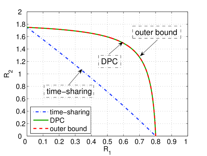
Figure 2: Comparison of the Sato-type outer bound and secrecy rate regions achieved by time-sharing and simplified DPC schemes for the example MGBC-CM in (39)

Fig. 2 depicts inner and outer bounds on the secrecy capacity for the example MGBC-CM described in (39). We compare the Sato-type outer bound (indicated by the dashed line) with the secrecy rate regions achieved by the simplified DPC coding scheme (indicated by the solid line) and the time-sharing scheme (indicated by the dash-dot line). Surprisingly, we observe that not only the corner points but also the boundary of the simplified DPC secrecy rate region (36) is identical with the Sato-type outer bound (17). Furthermore, Fig. 2 demonstrates that the time-sharing scheme is strictly suboptimal for providing the secrecy capacity region.

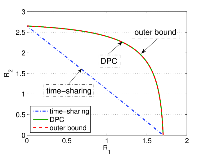
Figure 3: Comparison of the Sato-type outer bound and secrecy rate regions achieved by time-sharing and simplified DPC schemes for the example MGBC-CM in (40)

In the second example, we consider a broadcast channel with a small $\alpha$

$$y_{1} =s_{1}+\widetilde{z}_{1}$$

$$y_{2} =2(0.2s_{1}+\sqrt{1-0.04}s_{2})+\widetilde{z}_{2}$$ (40)

i.e., $|\widetilde{\mathbf{h}}|=1$, $|\widetilde{\mathbf{g}}|=2$ and $\alpha=0.2$. The total power $A=10$. Fig. 3 illustrates that, again, the boundary of the simplified DPC secrecy rate region (36) is consistent with the Sato-type outer bound (17).

6 Conclusion

In this paper, we have investigated outer and inner bounds on the secrecy capacity region of a generally non-degraded Gaussian broadcast channel with confidential messages for two users, where the transmitter has $t$ antennas and each user has one antenna. For this model, we have introduced a computable Sato-type outer bound and proposed a dirty-paper secure coding scheme. Using numerical examples, we have illustrated that the boundary of the simplified DPC secrecy rate region is consistent with the Sato-type outer bound.

Based on this observation, we conjecture that the dirty-paper secure coding strategy achieves the secrecy capacity region of the MGBC-CM.

Appendix

Proof

(Theorem 3.1) Here we prove Theorem 3.1 and derive the outer bound for $R_{1}$. The outer bound for $R_{2}$ follows by symmetry.

The secrecy requirement (5) implies that

$$nR_{1}=H(W_{1}) \leq H(W_{1}|Y_{2}^{n},W_{2})+n\epsilon.$$ (41)

On the other hand, Fano’s inequality and $P_{e}\leq\epsilon$ imply that

$$H(W_{1}|Y_{1}^{n}) \leq\epsilon\log(M_{1}-1)+h(\epsilon)\triangleq n\delta_{1}.$$ (42)

where $h(x)$ is the binary entropy function. Now, we can bound (41) as follows

$$nR_{1} \leq H(W_{1}|Y_{2}^{n})+n\epsilon$$ (43)

$$\leq H(W_{1}|Y_{2}^{n})-H(W_{1}|Y_{1}^{n})+n(\delta_{1}+\epsilon)$$ (44)

$$\leq H(W_{1}|Y_{2}^{n})-H(W_{1}|Y_{1}^{n},Y_{2}^{n})+n(\delta_{1}+\epsilon)$$ (45)

$$=I(W_{1};Y_{1}^{n}|Y_{2}^{n})+n(\delta_{1}+\epsilon)$$ (46)

$$\leq I(\mathbf{X}^{n};Y_{1}^{n}|Y_{2}^{n})+n(\delta_{1}+\epsilon)$$ (47)

$$\leq\sum_{i=1}^{n}I(\mathbf{X}_{i};Y_{1,i}|Y_{2,i})+n(\delta_{1}+\epsilon).$$ (48)

Note that the decoding error probability and the equivocation rate at each user depend only on the marginal probability densities $P(y_{1}|\mathbf{x})$ and $P(y_{2}|\mathbf{x})$. Hence, one can replace $Y_{1}$ and $Y_{2}$ by $\widetilde{Y}_{1}$ and $\widetilde{Y}_{2}$. Therefore, we have the desired result.

Proof

(Theorem 4.2) We first check the power constraint. Since $U_{1}$ and $U_{2}$ are independent and

$$\mathbf{s}=[s_{1},s_{2}]^{\top}=\mathbf{u}_{1}+\mathbf{u}_{2},$$

the covariance matrices $K_{U_{1}}$ and $K_{U_{2}}$ satisfy

$${\rm tr}(K_{U_{1}}+K_{U_{2}})={\rm tr}(K_{S_{1},S_{2}})\leq A.$$ (49)

Following from [19, Theorem 1] and using the setting in (23), we can immediately obtain the well-known successive encoding result:

$$I(V_{1};Y_{1}) =\log_{2}\frac{1+\widetilde{\mathbf{h}}^{H}(K_{U_{1}}+K_{U_{2}})\widetilde{\mathbf{h}}}{1+\widetilde{\mathbf{h}}^{H}K_{U_{2}}\widetilde{\mathbf{h}}}$$ (50)

and

$$I(V_{2};Y_{2})-I(V_{1};V_{2}) =\log_{2}(1+\widetilde{\mathbf{g}}^{H}K_{U_{2}}\widetilde{\mathbf{g}}).$$ (51)

Since $V_{1}=U_{1}$ is independent of $U_{2}$ and $V_{2}=U_{2}+\mathbf{b}\widetilde{\mathbf{g}}^{H}U_{1}$, we have

$$I(V_{2};Y_{1}|V_{1}) =I(U_{2}+\mathbf{b}\widetilde{\mathbf{g}}^{H}U_{1};\,Y_{1}|U_{1})$$

$$=I(U_{2};Y_{1}|U_{1})$$ (52)

$$=\log_{2}(1+\widetilde{\mathbf{h}}^{H}K_{U_{2}}\widetilde{\mathbf{h}}).$$ (53)

Moreover, we note that

$$I(V_{1};Y_{2}|V_{2})+I(V_{1};V_{2}) =I(V_{1},V_{2};Y_{2})-[I(V_{2};Y_{2})-I(V_{1};V_{2})]$$

$$=\log_{2}\frac{1+\widetilde{\mathbf{g}}^{H}(K_{U_{1}}+K_{U_{2}})\widetilde{\mathbf{g}}}{1+\widetilde{\mathbf{g}}^{H}K_{U_{2}}\widetilde{\mathbf{g}}}.$$ (54)

Substituting (50)-(54) into (18) and (19), we have the desired result.

References

• [1] A. D. Wyner, “The wire-tap channel,” Bell Syst. Tech. J., vol. 54, no. 8, pp. 1355–138, Oct. 1975.
• [2] I. Csiszár and J. Körner, “Broadcast channels with confidential messages,” IEEE Trans. Inf. Theory, vol. 24, no. 3, pp. 339–348, May 1978.
• [3] Y. Oohama, “Coding for relay channels with confidential messages,” in Proc. IEEE Information Theory Workshop, Cairns, Australia, Sep. 2001, pp. 87–89.
• [4] I. Csiszár and P. Narayan, “Secrecy capacities for multiple terminal,” IEEE Trans. Inf. Theory, vol. 50, no. 12, pp. 3047–3061, Dec 2004.
• [5] E. Tekin and A. Yener, “The Gaussian multiple access wire-tap channel with collective secrecy constraints,” in Proc. IEEE Int. Symp. Information Theory (ISIT), Seattle, USA, Jul. 2006.
• [6] Y. Liang and H. Vincent Poor, “Generalized multiple access channels with confidential messages,” IEEE Trans. Inf. Theory, submitted (under revision), April 2006. [Online]. Available: http://arxiv.org/PS$_$cache/cs/pdf/0605/0605014.pdf
• [7] R. Liu, I. Maric, R. D. Yates, and P. Spasojevic, “The discrete memoryless multiple access channel with confidential messages,” in Proc. IEEE Int. Symp. Information Theory (ISIT), Jul. 2006, pp. 957 – 961.
• [8] R. Liu, I. Maric, P. Spasojevic, and R. Yates, “Discrete memoryless interference and broadcast channels with confidential messages,” in Proc. Allerton Conference on Communication, Control, and Computing, Sep. 2006.
• [9] L. Lai and H. El Gamal, “The relay-eavesdropper channel: Cooperation for secrecy,” IEEE Trans. Inf. Theory, submitted, Dec. 2006.
• [10] Z. Li, W. Trappe, and R. Yates, “Secret communication via multi-antenna transmission,” in Proc. Forty-First Annual Conference on Information Sciences and Systems (CISS), Baltimore, MD, USA, Mar. 2007.
• [11] T. Cover and J. Thomas, Elements of Information Theory.   New York: John Wiley Sons, Inc., 1991.
• [12] S. K. Leung-Yan-Cheong and M. E. Hellman, “The Gaussian wire-tap channel,” IEEE Trans. Inf. Theory, vol. 24, no. 4, pp. 51–456, Jul. 1978.
• [13] R. Liu, I. Maric, P. Spasojevic, and R. Yates, “Discrete memoryless interference and broadcast channels with confidential messages: Secrecy rate regions,” IEEE Trans. Inf. Theory, submitted, Feb 2007. [Online]. Available: http://arxiv.org/PS$_$cache/cs/pdf/0702/0702099.pdf
• [14] K. Marton, “A coding theorem for the discrete memoryless broadcast channel,” IEEE Trans. Inf. Theory, vol. 25, pp. 306–311, May 1979.
• [15] D. Slepian and J. K. Wolf, “Noiseless coding of correlated information sources,” IEEE Trans. Inf. Theory, vol. 19, no. 4, pp. 471–480, Jul. 1973.
• [16] S. I. Gel’fand and M. S. Pinsker, “Coding for channel with random parameters,” Problemy Peredachi Informatsii, vol. 9, pp. 19–31, 1980.
• [17] M. Costa, “Writing on dirty paper,” IEEE Trans. Inf. Theory, vol. 29, pp. 439–441, May 1983.
• [18] A. Khisti, G. Wornell, A. Wiesel, and Y. Eldar, “On the Gaussian MIMO wiretap channel,” in Proc. IEEE Int. Symp. Information Theory (ISIT), to appear, Nice, France, Jun. 2007.
• [19] W. Yu and J. M. Cioffi, “Sum capacity of Gaussian vector broadcast channels,” IEEE Trans. Inf. Theory, vol. 50, pp. 1875–1892, Sep. 2004.