Puzzles, Tableaux, and Mosaics

Abstract

We define mosaics, which are naturally in bijection with Knutson-Tao puzzles. We define an operation on mosaics, which shows they are also in bijection with Littlewood-Richardson skew-tableaux. Another consequence of this construction is that we obtain bijective proofs of commutativity and associativity for the ring structures defined either of these objects. In particular, we obtain a new, easy proof of the Littlewood-Richardson rule. Finally we discuss how our operation is related to other known constructions, particularly jeu de taquin.

1 Introduction

It is well known that the cohomology ring of the Grassmannian $\mathcal{H}_{d,n}:=H^{*}(Gr(d,n))$ has a natural geometric basis, the Schur basis $\{s_{\lambda}\ |\ \lambda\in\Lambda\}$. The structure constants $a_{\nu\mu}^{\lambda}$ of $\mathcal{H}_{d,n}$ in the Schur basis, defined by

$$s_{\nu}s_{\mu}=\sum_{\lambda\in\Lambda}a_{\nu\mu}^{\lambda}s_{\lambda}\,,$$

are the Littlewood-Richardson numbers. They are non-negative integers, and also appear as structure constants in representation ring of $GL(d)$ and the ring of symmetric polynomials.

Throughout, the integers $0<d<n$, will be fixed. The set $\Lambda$ which indexes the Schur classes $s_{\lambda}\in\mathcal{H}_{d,n}$ can be viewed concretely as either the set of $01$-strings of length $n$ with, with exactly $d$ ones, or as partitions whose diagram fits inside a $d\times n{-}d$ rectangle. There is a standard way of passing back and forth between these two: the positions of the zeroes and ones in a $01$-string are respectively the positions of the horizontal and vertical steps along the boundary of the corresponding diagram, as shown below.

An important problem of the last century has been to find combinatorial interpretations for the Littlewood-Richardson numbers; we refer to these collectively as Littlewood-Richardson rules. In this paper we shall be concerned with two such rules. The first, due to Knutson, Tao and Woodward, states that $a_{\nu\mu}^{\lambda}$ can be obtained by counting puzzles with $\nu$, $\mu$ and $\lambda$ on the boundary [KTW1]. The second is the original Littlewood-Richardson rule [LR], which was proved in [S], and states that $a_{\nu\mu}^{\lambda}$ can be obtained by counting Littlewood-Richardson tableaux (LR-tableaux). We recall these rules and all relevant definitions in Sections 2.1 and 2.2.

The purpose of this paper is to introduce a new construction—mosaics—which will allow us to give new simple proofs of both of these rules, and provide a bijection between them. To show that a Littlewood-Richardson rule is correct, one needs to check two things:

1. that the numbers given by the rule are the structure constants of a commutative, associative ring;

2. that the Pieri rule holds, that is, multiplication by special classes which are generators of $\mathcal{H}_{d,n}$ behaves correctly.

The Pieri rule is fairly trivial to check for both puzzles and tableaux. (The rule simply states that $a_{(k)\,\mu}^{\ \lambda}=1$ if the diagram $\lambda/\mu$ consists of $k$ boxes in $k$ distinct columns, and equals zero otherwise, where $(k)$ is the partition $k\geq 0\geq\cdots\geq 0$; the classes $\{s_{(k)}\}_{k\leq n-d}$ generate $\mathcal{H}_{d,n}$.) Our focus, therefore, will be on proving commutativity and associativity. N.B. Although we shall prove both here, to prove a Littlewood-Richardson rule, associativity alone is sufficient.

This approach of showing Pieri and associativity was used by Knutson, Tao and Woodward to give a proof of the hive formulation of the Littlewood-Richardson rule [KTW2]. From this, one can deduce the puzzle rule. For LR-tableaux, it is possible to prove commutativity and associativity using tableau switching, as defined in [BSS]. While this approach to showing commutativity has been discovered many times, the fact that one can also show associativity (Corollary 3.6) in this way does not appear to be well documented. Buch, Kresch, and Tamvakis, also gave simple, parallel proofs of the Littlewood-Richardson rule and the puzzle rule along these lines [BKT]. Our approach is unique in that the worlds of puzzles and tableaux are intertwined, the result of which is that our proofs are surprisingly short and clean.

Because puzzles have a three-fold symmetry, it will be more convenient phrase statements of commutativity and associativity in terms of symmetric Littlewood-Richardson numbers, which are defined to be

$$a_{\nu\mu\lambda^{\vee}}:=\int_{Gr(d,n)}s_{\nu}s_{\mu}s_{\lambda^{\vee}}\,.$$

These are related to the ordinary Littlewood-Richardson numbers by the fact that $a_{\nu\mu\lambda^{\vee}}=a_{\nu\mu}^{\lambda}$, where $s_{\lambda^{\vee}}$ is the unique Schur class such that

$$\int_{Gr(d,n)}s_{\lambda}s_{\lambda^{\vee}}=1\,.$$

In terms of partitions, $\lambda^{\vee}$ is the complement of $\lambda$; in terms of $01$-strings, $\lambda^{\vee}$ is the reverse of $\lambda$. Commutativity of $\mathcal{H}_{d,n}$ is expressed by the statement that

$$a_{\nu\mu\lambda^{\vee}}=a_{\mu\nu\lambda^{\vee}}\,,$$ (1)

and associativity is expressed as

$$\sum_{\kappa\in\Lambda}a_{\nu\mu\kappa^{\vee}}\,a_{\xi\kappa\lambda^{\vee}}=\sum_{\kappa\in\Lambda}a_{\mu\xi\kappa^{\vee}}\,a_{\kappa\nu\lambda^{\vee}}\,.$$ (2)

1.1 Preliminary examples

Mosaics are certain tilings of a hexagonal region. One can regard a mosaic as a crooked drawing of a puzzle with some extra rhombi in the corners; in fact, there is a straightforward bijection (c.f. Section 2.4) between mosaics and puzzles, obtained by removing the extra rhombi, and straightening. Figure 1 illustrates an example of a mosaic and the corresponding puzzle under this bijection.

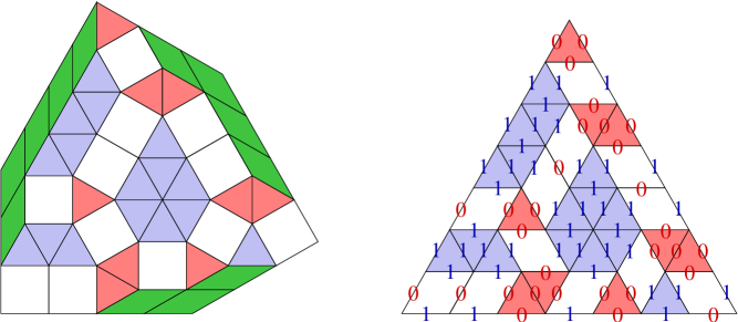
Figure 1: A mosaic with $n=7$, $d=4$, and the corresponding puzzle.

The big advantage of mosaics over puzzles is the fact that these extra rhombi are arranged in the shape of a (slightly distorted) Young diagram. We define flocks, which are tableau-like structures on the rhombi, and an operation called migration on flocks. Our main results state that migration is an invertible operation which preserves the flock structure. Thus migration allows us to move flocks around inside a mosaic without losing any information.

Figure 2 illustrates an example of a flock on the left side of a mosaic migrating to the right side. The result of such a migration is that the flock assumes a shape which can be interpreted as an LR-tableau, in this case migration identifies the initial mosaic with the LR-tableau

 .

Our main theorems imply that this process gives a bijection between mosaics (or equivalently puzzles) and LR-tableaux.

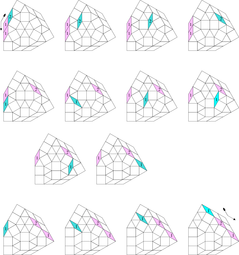
Figure 2: A flock migrates from the left side of the mosaic to the right.

One can also perform a sequence of migrations to swap the positions of two flocks inside a mosaic. This allows us to deduce that the product structure on $\mathcal{H}_{d,n}$ defined by puzzles is commutative. Similar types of arguments allow us to prove commutativity and associativity for both puzzles and LR-tableaux.

1.2 Outline

This paper is organised as follows. In Section 2, we recall the relevant background information on puzzles and tableaux, and introduce flocks and mosaics. The migration operation is defined in Section 3. From here, we give the precise statement of our main theorems, and the details of how commutativity and associativity follow as a consequence. We prove the main theorems in Section 4. Finally, in Section 5 we discuss how migration is related to other known constructions, particularly to jeu de taquin. With the exception of this last section, we have attempted to keep the exposition entirely self-contained.

We would also like to warn the reader that all directions in this paper are used in a relative, rather than in an absolute sense. When we speak of “up”, “down”, “left” and “right”, these are defined relative to a chosen “right”; hence the reader may sometimes need to rotate the page so that these are pointing in their usual direction. Compass directions “north”, “east”, “south” and “west”, are used even more loosely. These are defined relative to a chosen basis for $\mathbb{R}^{2}$, which may not be orthogonal or even have the expected orientation. Hence, east and right are not always the same direction, and even if they are, north and up need not be the same. In Sections 2.1 and 2.2 these directions have their usual meanings, but thereafter we will need this additional flexibility.

1.3 Acknowledgements

The author is grateful to Allen Knutson for helpful comments on the paper, and to the Banff International Research Station for providing the inspirational surroundings in which these ideas were hatched. This research was partially supported by NSERC.

2 Background and definitions

2.1 Puzzles

A puzzle of size $n$ is a tiling of an equilateral triangle of side length $n$, using the following pieces (each has unit side length)

subject to the following conditions:

1. the pieces can be rotated in any orientation, but not reflected;

2. wherever two pieces share an edge, the numbers on the edge must agree.

If we read the numbers on the boundary of a puzzle, clockwise starting from the lower-left corner, we see three strings of $0$s and $1$s, $\pi$, $\rho$, $\sigma$ of length $n$. See Figure 3 (left). We call $(\pi,\rho,\sigma)$ the boundary data of the puzzle. For a string $\sigma=\sigma_{1}\ldots\sigma_{n}$, let $\sigma^{\vee}=\sigma_{n}\ldots\sigma_{1}$ denote its reversal.

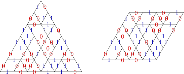
Figure 3: A puzzle with boundary data $(001101,010101,011001)$ and a bipuzzle with boundary data $(0101,0101,0011,1001)$.

We recall the following basic fact about puzzles:

Proposition 2.1.

If $(\pi,\rho,\sigma)$ is the boundary of a puzzle, then the strings $\pi$, $\rho$ and $\sigma$ have the same number of $1$s.

Henceforth, we shall assume this number equals $d$.

Let $b_{\pi\rho\sigma}$ denote the number of puzzles with boundary data $(\pi,\rho,\sigma)$. The puzzle-theoretic Littlewood-Richardson rule states $b_{\pi\rho\sigma}=a_{\pi\rho\sigma}$.

A bipuzzle is a tiling of the rhombus of side length $n$ with angles $60^{\circ}$ and $120^{\circ}$, satisfying conditions (i), (ii) and

1. the number of $1$s appearing on each side of the rhombus is equal to the number on any other side.

Again, we assume that this number is equal to $d$. The boundary data of a bipuzzle is the list of strings $(\pi,\rho,\sigma,\tau)$ read clockwise from the lower-left corner. See Figure 3 (right).

We will need the following fact.

Proposition 2.2.

Every bipuzzle can be split in half into two single puzzles.

In other words, there are no rhombi that lie across the line which divides the bipuzzle into two equilateral triangles of side length $n$. This has an easy “Green’s theorem” style proof, as in [KT2, Lemma 5]; we also give an alternate proof in Section 4. Bipuzzles are important for associativity (c.f. (2)), as we have:

Proposition 2.3.

The number of bipuzzles with boundary data $(\pi,\rho,\sigma,\tau)$ is equal to $\sum_{\upsilon\in\Lambda}b_{\rho\sigma\upsilon^{\vee}}\,b_{\pi\upsilon\tau}=\sum_{\upsilon\in\Lambda}b_{\rho\sigma\upsilon^{\vee}}\,b_{\upsilon\tau\pi}$.

Proof.

First note that the two sums are equal, since by the rotational symmetry of the puzzle rule, $b_{\pi\upsilon\tau}=b_{\upsilon\tau\pi}$. The expression $\sum_{\upsilon\in\Lambda}b_{\rho\sigma\upsilon^{\vee}}\,b_{\pi\upsilon\tau}$ counts pairs of puzzles with boundary data $(\pi,\upsilon,\tau)$ and $(\rho,\sigma,\upsilon^{\vee})$ for some $\upsilon\in\Lambda$. But any such pair can be glued along the $\upsilon$-boundary to form a bipuzzle with boundary data $(\pi,\rho,\sigma,\tau)$, and by Proposition 2.2 every bipuzzle arises in this way. ∎

2.2 Young tableaux

A partition $\lambda=\lambda_{1}\geq\dots\geq\lambda_{d}\geq 0$ is a decreasing sequence of integers. We will assume that all of our partitions have at most $d$ parts, and that $\lambda_{1}\leq n-d$. The complement of $\lambda$ is the partition $\lambda^{\vee}=\lambda^{\vee}_{1}\geq\cdots\geq\lambda^{\vee}_{d}\geq 0$, having parts $\lambda^{\vee}_{k}=n-d-\lambda_{d-k}$.

To each partition $\lambda$, we associate its diagram, also denoted $\lambda$. We adopt the French convention, in which the southmost row has $\lambda_{1}$ boxes, the next higher row has $\lambda_{2}$ boxes, etc. All rows are assumed to be left justified. The conjugate of $\lambda$ is the partition $\lambda^{t}$ whose diagram has whose diagram has $\lambda_{k}$ boxes in the $k^{\text{th}}$ column. A skew diagram $\lambda/\mu$ is the diagram consisting of all boxes of $\lambda$, which are not also boxes of the subdiagram $\mu$. Here we assume, of course, that $\mu$ and $\lambda$ have the same southwest corner. We sometimes refer to a partition diagram as a straight diagram, to emphasize that it is non-skew.

For any skew diagram $\lambda/\mu$, a Littlewood-Richardson tableau (or LR-tableau), is a function $f$ which assigns positive integer entries to the boxes of $\lambda/\mu$ such that:

1. the entries are weakly increasing in each row from east to west;

2. the entries are strictly increasing in each column from south to north;

3. if one forms the word $w_{1}\ldots w_{r}$ by listing the entries in the ordinary reading order (west to east and north to south), then for all $k\geq 1$, each tail subword $w_{s}\ldots w_{r}$ has at least as many $k$s as $(k{+}1)$s.

Given an LR-tableau $f$, the standard order on the boxes is the following: $X<_{f}Y$ iff either $f(X)<f(Y)$, or $f(X)=f(Y)$ and $X$ is west (or northwest) of $Y$. This ordering will be key for us. It arises in other contexts in tableau theory, for example in defining Schützenberger slides.

The content of a LR-tableau is the partition $\nu=\nu_{1}\geq\dots\geq\nu_{r}$, where $\nu_{k}$ is the number of $k$s in the tableau. The boundary data of a LR-tableau of shape $\lambda/\mu$ and content $\nu$ are defined to be $(\nu,\mu,\lambda^{\vee})$.

Let $c_{\nu\mu\lambda^{\vee}}$ denote the number of LR-tableaux with boundary data $(\nu,\mu,\lambda^{\vee})$. The Littlewood-Richardson rule asserts that $c_{\nu\mu\lambda^{\vee}}=a_{\nu\mu\lambda^{\vee}}$.

An LR-bitableau on a skew diagram $\lambda/\mu$ is partition diagram $\kappa$ with $\mu\subset\kappa\subset\lambda$ together with a pair of LR-tableaux $f$ and $g$ on $\lambda/\kappa$ and $\kappa/\mu$. The boundary data of this LR-bitableau are $(\xi,\nu,\mu,\lambda^{\vee})$, where $\xi$ and $\nu$ are the content of $f$ and $g$ respectively. LR-bitableaux are important for associativity (c.f. (2)), since we have:

Proposition 2.4.

The number of LR-bitableaux with boundary data $(\xi,\nu,\mu,\lambda^{\vee})$ is $\sum_{\kappa\in\Lambda}c_{\nu\mu\kappa^{\vee}}\,c_{\xi\kappa\lambda^{\vee}}$.

2.3 Transformed tableaux and flocks

When we introduce mosaics, we will encounter pictures which look like skew diagrams that have been subjected to a linear transformation. We refer to such a picture as a transformed diagram. We would like to treat transformed diagrams as standard skew diagrams. However, without knowing the linear transformation, we cannot uniquely determine the original skew diagram from the transformed diagram—there can be (and usually are) up to four possibilities. We therefore define an orientation on a transformed diagram $\alpha$ to be a pair of vectors $E,N\in\mathbb{R}^{2}$, such that if $\phi$ is the linear transformation given by the matrix $(E|N)$, then $\phi^{-1}(\alpha)$ is a standard skew diagram. An orientation gives a concrete identification of a transformed diagram with a standard skew diagram. To specify and orientation pictorially, we draw $E$ with a single headed arrow, and $N$ with a double headed arrow, as shown below. (The arrowheads reflect the fact that the entries of an LR-tableau weakly increase eastward and strictly increase northward.)

Henceforth we will refer to the directions $E$, $N$, $-E$, $-N$ as east, north, west and south, respectively. Once an orientation has been chosen, we can talk about LR-tableaux, standard order, etc. on a transformed diagram—our existing definitions make sense once the compass directions are thusly redefined.

A nest is a designated convex cone in the plane, with angle $150^{\circ}$. An orientation on a nest is a pair of unit vectors $(E,N)$ parallel to the sides of the cone at an angle of $150^{\circ}$. There are four possible orientations for any nest. Consider a collection of rhombi of unit side length with angles $150^{\circ}$ and $30^{\circ}$. We say that the rhombi are packed in the nest, if they lie inside the cone, have edges parallel to the cone, and are a linear transformation of a straight diagram whose corner is the corner of the cone.

Figure 4: Three collections of rhombi packed in nests; (a) and (b) are equivalent, while (c) is a complement to both (a) and (b) when $d=4$, $n=9$.

Given two collections of rhombi $\alpha$ and $\beta$ packed in two different nests, we say that $\alpha$ is equivalent to $\beta$ if there is an orientation preserving isometry which maps one to the other. We say that $\alpha$ is a complement of $\beta$, written $\alpha=\beta^{\vee}$, if there is an orientation preserving isometries $\phi_{1},\phi_{2}$ such that $\phi_{1}(\alpha)$ and $\phi_{2}(\beta)$ do not overlap, and together tile the $d\times n{-}d$ parallelogram below. See Figure 4.

Given a collection of rhombi $\alpha$ packed in a nest, a triple $F=(\zeta,(E,N),f)$ is called a flock (on $\zeta$) if

1. $\zeta\subset\alpha$ is a subset of these rhombi, in the shape of a transformed diagram;

2. $(E,N)$ is an orientation for both the nest and for $\zeta$;

3. $f:\zeta\to\mathbb{N}$ is an LR-tableau on $\zeta$ in this orientation.

The content of a flock is the content of $f$. If $\alpha$ is the set of all rhombi in the nest, we say that $F$ is accessible if $\zeta=\alpha/\alpha_{1}$ for some (transformed) straight diagram $\alpha_{1}\subset\alpha$. A single rhombus $\lozenge\in\alpha$ is accessible if the unique flock on $\{\lozenge\}$ is accessible.

Note if the nest has already been given an orientation, we do not insist that a flock have the same orientation. Thus we can have flocks of different orientations in the same nest.

2.4 Mosaics

Consider the hexagon $A^{\prime}AB^{\prime}BC^{\prime}C$ (vertices listed clockwise) which has angles $150^{\circ}$ at $A$, $B$, $C$, $90^{\circ}$ at $A^{\prime}$, $B^{\prime}$, $C^{\prime}$, and side lengths $A^{\prime}A=B^{\prime}B=C^{\prime}C=d$ and $AB^{\prime}=BC^{\prime}=CA^{\prime}=n-d$. where $0<d<n$ are integers. We designate three nests, at the corners $A$, $B$ and $C$. Define unit vectors $E_{A},N_{A},E_{B},N_{B},E_{C},N_{C}$ in the directions of $\overrightarrow{AA^{\prime}},\overrightarrow{AB^{\prime}},\overrightarrow{BB^{\prime}},\overrightarrow{BC^{\prime}},\overrightarrow{CC^{\prime}},\overrightarrow{CA^{\prime}}$ respectively, and fix orientations $(E_{A},N_{A})$, $(E_{B},N_{B})$, $(E_{C},N_{C})$ on the nests at $A$, $B$, and $C$ respectively. See Figure 5 (left).

Figure 5: The hexagon $A^{\prime}AB^{\prime}BC^{\prime}C$ and the octagon $A^{\prime}AB^{\prime}BC^{\prime}CD^{\prime}D$ and their nests, used in mosaics and bimosaics respectively.

A mosaic is a tiling of this hexagon by the following three shapes:
(a) the equilateral triangle with side length 1, (b) the square with side length 1, (c) the rhombus with side length 1, and angles $30^{\circ}$ and $150^{\circ}$,            
such that all rhombi are packed into the three nests of the hexagon. The collections of rhombi in nests $A$, $B$ and $C$ are denoted $\alpha$, $\beta$, $\gamma$ respectively, and $(\alpha,\beta,\gamma)$ are called the boundary data of the mosaic. The standard orientations on $\alpha,\beta,\gamma$ are the orientations of the nests $A$, $B$, and $C$ respectively.

There is a natural bijection between mosaics and puzzles, which easiest to describe physically. Take a mosaic and remove all the rhombi. Now imagine the corners of each square have hinges so that the angles of the square can flex to become a rhombus. Grab the three corners $A^{\prime}$, $B^{\prime}$, $C^{\prime}$ and pull tight in outward directions. The boundary will straighten into an equilateral triangle of side length $n$, and the squares will become $30^{\circ}$/$60^{\circ}$-rhombi. Finally note that some line segments will have rotated clockwise, while others will have rotated counterclockwise. This distinction gives the $0$s and $1$s on the puzzle, respectively. See Figure 1.

The proof that this works comes from an observation of Knutson and Tao (unpublished): puzzles are actually the projection of a unique piecewise linear surface in $\mathbb{R}^{4}$, where the edges point in directions $(1,0,0,0)$, $(0,1,0,0)$, $(1,-1,0,0)$ if the edge is labelled $0$, and $(0,0,1,0)$, $(0,0,0,1)$, $(0,0,1,-1)$ if the edge is labelled $1$. Mosaics are obtained from a slightly different projection, and the two projections are related by the operation just described.

This bijection shows us how to compare the boundary data of a puzzle with the boundary data of a mosaic. Under this bijection we see that the shape left by removing $\alpha$ turns into the string of $0$s and $1$s corresponding to the walk from $A^{\prime}$ to $B^{\prime}$: we get a $0$ for each unit step west, and a $1$ for each unit step north. We will say that a mosaic with boundary data $(\alpha,\beta,\gamma)$ and a puzzle with boundary data $(\pi,\rho,\sigma)$ have the same boundary, if this correspondence identifies $\alpha$ with $\pi$, $\beta$ with $\rho$ and $\gamma$ with $\sigma$. We will write $b_{\alpha\beta\gamma}=b_{\pi\rho\sigma}$ for the number of puzzles with boundary data $(\alpha,\beta,\gamma)$.

We can also easily compare the boundary data of an LR-tableau and a mosaic. We will say that an mosaic with boundary data $(\alpha,\beta,\gamma)$ and an LR-tableau with boundary data $(\nu,\mu,\lambda^{\vee})$ have the same boundary, if the standard orientations identify $\alpha$ with $\nu$, $\beta$ with $\mu$ and $\gamma$ with $\lambda^{\vee}$. Note that these identifications are consistent with the bijection between partitions and $01$-strings described in Section 1.

We also define bimosaics, which (by the same straightening operation) naturally correspond to bipuzzles. Consider the octagon $A^{\prime}AB^{\prime}BC^{\prime}CD^{\prime}D$ (Figure 5 (right)) with angles $150^{\circ}$ at $A$, $B^{\prime}$, $B$, $C$, $D$, $D^{\prime}$ and $90^{\circ}$ at $A^{\prime}$, $C^{\prime}$, and side lengths $A^{\prime}A=B^{\prime}B=C^{\prime}C=D^{\prime}D=d$, $AB^{\prime}=BC^{\prime}=CD^{\prime}=DA^{\prime}=n-d$. We designate corners $A$, $B$, $C$ and $D$ to be nests. See Figure 5 (right). A bimosaic is a tiling of the octagon by the same three shapes as a mosaic, with all rhombi packed into the four nests. The boundary data of a bimosaic is $(\alpha,\beta,\gamma,\delta)$, the collections of rhombi at $A$, $B$, $C$, and $D$ respectively.

2.5 Canonical constructions

In a few key situations, certain objects are uniquely constructible. The following statements correspond to the fact that multiplying by identity element in $\mathcal{H}_{d,n}$ is trivial. We omit the proofs as they are straightforward, but illustrative examples are given in Figures 6 and 7.

Lemma 2.5.

Suppose we are give a nest with an orientation $(E,N)$. If $\alpha$ is packed in the nest, there is a unique function $f$ which makes $F=(\alpha,(E,N),f)$ a flock. Moreover for any partition $\nu$ there is a unique $\alpha$ such that this flock has content $\nu$. If the orientation is changed to $(-E,-N)$, the unique flock $F^{-}=(\alpha,(-E,-N),f^{-})$ has the same content as $F$. One of these two orientations identifies $\alpha$ with the content of $F$.

Figure 6: The unique flocks on a set of rhombi packed into a nest, under the orientations $(E,N)$ and $(-E,-N)$. In both cases the flock has content $(4,4,2,1,1)$.

Lemma 2.6.

If $\alpha=\varnothing$, then for any $\beta$, there is a unique mosaic with boundary data $(\alpha,\beta,\gamma)$. In this mosaic $\gamma$ is the complement of $\beta$. The same is true if the roles of $\alpha,\beta,\gamma$ are permuted.

Figure 7: The unique mosaic when with boundary data $(\varnothing,\beta,\beta^{\vee})$. Here $n=8$, $d=5$, and $\beta=2\geq 2\geq 1\geq 0\geq 0$ in the standard orientation.

3 Operations on mosaics

3.1 Migration

Migration is an operation which makes sense on both mosaics and bimosaics. The operation of migration takes an accessible flock and moves all of its rhombi in roughly one of four possible compass directions (e.g. north), so that the flock ends up in a different nest.

The input data for the operation of migration is therefore: (i) a mosaic or a bimosaic; (ii) an accessible flock $F=(\zeta,(E,N),f)$, where $\zeta$ is a collection of rhombi inside the (bi)mosaic; (iii) a compass direction, either $\text{north}=N$, $\text{east}=E$, $\text{south}=-N$ or $\text{west}=-E$. The compass direction must be consistent with the orientation of the flock, in the following sense: if the nest in which $F$ is contained opens to the northeast in this orientation of the flock, the direction must be either north or east; otherwise it must be south or west.

In describing migration we will assume that our diagrams are turned so that the direction of migration is pointing directly to our right. In the example of Figure 2, the direction of migration is north, and thus the page should be turned $60^{\circ}$ clockwise.

For north or east migration, we begin by locating the rhombus in $\zeta$ which is maximal in the standard order. For south or west migration, we locate the minimal one. Beginning with this rhombus and proceeding in the standard order (from largest to smallest, or the reverse, whichever is appropriate), we perform the following operation with each rhombus $\lozenge$ in turn:

Looking to the right of the rhombus $\lozenge$, find the smallest hexagon in which $\lozenge$ is contained. (There is always a unique minimal hexagon which is entirely weakly right of the leftmost point on $\lozenge$, though sometimes it may seem to be better described as above or below $\lozenge$.) Up to rotation and reflection, there are two possible things we could see:

If we see (a), the hexagon has a 2-fold rotational symmetry, so we rotate the tiling of this hexagon by $180^{\circ}$. If we see (b), the hexagon has a 3-fold rotational symmetry, so we rotate the tiling $120^{\circ}$, in whichever way causes some edge of the rhombus to end up exactly horizontal, or exactly vertical. (This restriction rules out one of two the possible $120^{\circ}$ rotations.) In this way, the rhombus moves roughly to the right (although sometimes it moves strictly vertically). Repeat this process, until the rhombus is packed into a new nest. Let $\lozenge^{\prime}$ denote the rhombus in its final position, and let $\zeta^{\prime}=\{\lozenge^{\prime}\ |\ \lozenge\in\zeta\}$ denote the collection of rhombi from $\zeta$ after migration.

Proposition 3.1.

All rhombi in $\zeta^{\prime}$ are in the same nest. Consequently, $\zeta^{\prime}$ is a transformed diagram.

Proof.

For single (hexagonal) mosaics this is clear, as the rhombi can only ever be in two of three orientations during the migration process, thereby ruling out one of the nests. This argument also works in bimosaics for migration towards the opposite nest. For the other case (migration towards the near nest), Proposition 2.2 implies that such a migration will behave as it does on a single mosaic. ∎

In light of this we can specify a direction of migration by specifying the target nest, rather than the compass direction. Note that in a bimosaic, we cannot migrate directly from $A$ to $B$, or $C$ to $D$, or vice versa.

There is an induced orientation $(E^{\prime},N^{\prime})$ on the transformed diagram $\zeta^{\prime}$ which is obtained by rotating the pair $(E,N)$ at most $60^{\circ}$. We also have a obvious function $f^{\prime}:\zeta^{\prime}\to\mathbb{N}$, which is defined by $f^{\prime}(\lozenge^{\prime})=f(\lozenge)$. Let $F^{\prime}$ denote the triple $(\zeta^{\prime},(N^{\prime},E^{\prime}),f^{\prime})$,

We can now state our main results.

Theorem 1.

If $F^{\prime}=(\zeta^{\prime},(N^{\prime},E^{\prime}),f^{\prime})$ is the result of migrating a flock $F=(\zeta,(N,E),f)$ in some direction inside a mosaic or a bimosaic, then $F^{\prime}$ is a flock. Moreover the map $\lozenge\mapsto\lozenge^{\prime}$ preserves the standard order.

Theorem 2.

Migration is an invertible operation. The inverse operation to the migration of a flock $F$ from a nest $A$ to a nest $B$ is the migration of $F^{\prime}$ from $B$ to $A$. Inverting, one recovers both the original flock and the original mosaic.

The proofs are given in Section 4. The remainder of this section will be devoted to corollaries of these theorems.

Note: because orientations can become rotated during migration, migration south is not necessarily the inverse of migration north. If the orientation is not rotated (i.e. $E=E^{\prime}$), then north and south migration are mutually inverse, as are east and west migration. Otherwise, north and west migration are mutually inverse, as are east and south migration. In single mosaics, only the latter case occurs.

3.2 Bijections between mosaics and tableaux

Corollary 3.2.

Migration gives a bijection between mosaics and LR-tableaux with the same boundary.

Proof.

Given a mosaic, with boundary data $(\alpha,\beta,\gamma)$, give $\alpha$ the orientation $(-E_{A},-N_{A})$ and form the unique flock $F=(\alpha,(-E_{A},-N_{A}),f)$. Let $F$ migrate from $A$ to $B$ (south). The resulting flock $F^{\prime}$ is identified with an LR-tableau, which (as one can easily check) has the correct boundary data.

The process is reversible. Given an LR-tableau of shape $\lambda/\mu$, form the unique mosaic with boundary data $(\varnothing,\gamma^{\vee},\gamma)$, where $\gamma^{\vee}$ is identified with $\lambda$. Now identify the tableau on $\lambda/\mu$ with a flock $G$ in $\gamma^{\vee}$. Let $G$ migrate from $B$ to $A$ (east) to obtain a new mosaic.

The two operations are inverse to each other: migration south is inverse to migration east, and the reconstruction of the forgotten data is always unique. ∎

By giving the flock on $\alpha$ different orientations, we obtain variants on this bijection. These are summarised in Table 1. The second of these bijections is essentially the same as Tao’s “proof without words” bijection which appears in [V]. We discuss this further in Section 5.1.

Orientation on $\alpha$	Mosaics with boundary data $(\alpha,\beta,\gamma)$ $\leftrightarrow$
$(-E_{A},-N_{A})$	LR-tableaux with (same) boundary data $(\nu,\mu,\lambda^{\vee})$
$(E_{A},N_{A})$	LR-tableaux with boundary data $(\nu,\lambda^{\vee},\mu)$
$(-N_{A},-E_{A})$	LR-tableaux with boundary data $(\nu^{t},\mu^{t},(\lambda^{\vee})^{t})$
$(N_{A},E_{A})$	LR-tableaux with boundary data $(\nu^{t},(\lambda^{\vee})^{t},\mu^{t})$

Table 1: Variants on the bijection in the proof of Corollary 3.2 obtained by changing the orientation on $\alpha$.

3.3 Commutativity

In the language of puzzles or mosaics, the statement that the multiplication on $\mathcal{H}_{d,n}$ is commutative, is the following.

Corollary 3.3.

There is a bijection between mosaics with boundary data $(\alpha,\beta,\gamma)$ and those with boundary data $(\beta,\alpha,\gamma)$.

Proof.

Fix any orientations on the nests $A$ and $B$ (not necessarily the standard ones). Given a mosaic with boundary data $(\alpha,\beta,\gamma)$, form the unique flocks $F$ and $G$ on $\alpha$ and $\beta$ with these orientations. Migrate $F$ from $A$ to $C$ to form $F^{\prime}$. Migrate $G$ from $B$ to $A$ to form $G^{\prime}$. Finally migrate $F^{\prime}$ from $C$ to $B$ to form $F^{\prime\prime}$. Since migration does not change the content of a flock, $F$ and $F^{\prime\prime}$ have the same content, and thus $\alpha$ and $\alpha^{\prime\prime}$ must be equivalent. Similarly, $\beta$ and $\beta^{\prime}$ are equivalent. Thus the result of this operation will have boundary data $(\beta,\alpha,\gamma)$.

The process yields new a orientation on $B$ coming from $F^{\prime\prime}$, which is a $120^{\circ}$ clockwise rotation of the original orientation on $A$, and a new orientation on $A$ coming from $F^{\prime}$, which is a $60^{\circ}$ counterclockwise rotation of the original orientation on $B$. Starting from these orientations, we can reverse the entire process and recover the original mosaic. Thus this map is a bijection. ∎

For tableaux, commutativity of $\mathcal{H}_{d,n}$ is expressed as follows.

Corollary 3.4.

There is a bijection between LR-tableaux with boundary data $(\nu,\mu,\lambda^{\vee})$ and those with boundary data $(\mu,\nu,\lambda^{\vee})$.

Proof.

Given a LR-tableau $f$ on $\lambda/\mu$ with content $\nu$, form the unique mosaic with boundary data $(\varnothing,\gamma^{\vee},\gamma)$, where $\gamma^{\vee}$ is identified with $\lambda$. Let $F=(\zeta,(E_{B},N_{B}),f)$ be the flock in $\gamma^{\vee}$ corresponding to $f$. Also, let $\eta\subset\gamma^{\vee}$ be the subset corresponding to $\nu$, and $G=(\eta,(-E_{B},-N_{B}),g)$ be the unique flock on $\eta$. Migrate $F$ from $B$ to $A$, then migrate $G$ from $B$ to $A$. The resulting flocks $F^{\prime}$ and $G^{\prime}$ will be such that $G^{\prime}$ has boundary data ($\mu,\nu,\lambda^{\vee})$. As the nest at $B$ is now empty, this process is reversible. ∎

3.4 Associativity

By Proposition 2.3, associativity takes the following form for mosaics.

Corollary 3.5.

There is a bijection between bimosaics with boundary data $(\alpha,\beta,\gamma,\delta)$ and those with boundary data $(\delta,\alpha,\beta,\gamma)$.

Proof.

There are many ways to do this. One simply has to form flocks on $\alpha$, $\beta$, $\gamma$, and $\delta$ and shuffle them around appropriately inside a bimosaic. Again, the invertibility of such a shuffle operation relies on the fact that orientations rotate in predictable way under migration. ∎

The situation for tableaux is a little less clean, since we do not have the manifest rotational symmetry of the puzzle rule. The following assertion for LR-bitableaux does not precisely show associativity: by Proposition 2.4 it translates to the statement that $x(yz)=z(xy)$. This plus commutativity gives associativity.

Corollary 3.6.

There is a bijection between LR-bitableaux with boundary data $(\xi,\nu,\mu,\lambda^{\vee})$ and those with boundary data $(\nu,\mu,\xi,\lambda^{\vee})$

Proof.

An LR-bitableau with boundary data $(\xi,\nu,\mu,\lambda^{\vee})$ is a pair of LR-tableaux $f$ on $\lambda/\kappa$ with content $\xi$ and $g$ on $\kappa/\mu$ with content $\nu$. Given a such an LR-bitableau, form the unique mosaic with boundary data $(\varnothing,\gamma^{\vee},\gamma)$, where $\gamma^{\vee}$ is identified with $\lambda$. Let $F=(\zeta,(E_{B},N_{B}),f)$ be the flock in $\gamma^{\vee}$ corresponding to $f$. Let $G=(\eta,(E_{B},N_{B}),g)$ be the flock corresponding to $g$. Let $\theta\subset\gamma^{\vee}$ correspond to $\mu$ and let $H=(\theta,(-E_{B},-N_{B}),h)$ be the unique flock on $\theta$.

First migrate $F$ from $B$ to $A$. Then migrate $G$ from $B$ to $C$ to form $G^{\prime}$. Next, migrate $H$ from $B$ to $A$ to produce $H^{\prime}$, clearing out the nest at $B$. Finally migrate $G^{\prime}$ from $C$ to $A$ to produce $G^{\prime\prime}$ The resulting flocks $G^{\prime\prime}$ and $H^{\prime}$ together determine an LR-bitableau with boundary data $(\mu,\nu,\xi,\lambda^{\vee})$. As in the proof of commutativity, this is a bijection. ∎

4 Proof of main theorems

Once again, we describe our operations under the assumption that that the direction of migration is to our right.

Consider the journey of a single rhombus $\lozenge$ from one nest to another in the process of migration. The set of tiles (triangles and squares) that are displaced by this journey form a path from the initial position of $\lozenge$ to the final position $\lozenge^{\prime}$. We call the set of all these tiles the wake of $\lozenge$. This path is everywhere two tiles wide, and can be subdivided into two parallel paths, one directly above the other, each one tile wide. We call these the upper wake and lower wake of $\lozenge$. The line which divides them is called the midline of $\lozenge$. See Figure 8.

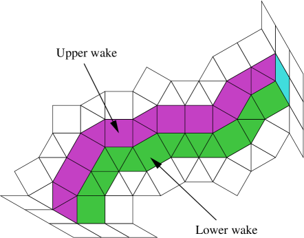
Figure 8: The upper and lower wakes, after the highlighted rhombus $\lozenge$ has migrated to the right.

Later in the process, when another rhombus $\begin{picture}(0.0,0.0)(0.0,0.0)\put(0.0,0.0){${\blacklozenge}$}\end{picture}\nolinebreak\lozenge$ takes its journey it may or may not displace some of the tiles in the wake of $\lozenge$. We will say that $\begin{picture}(0.0,0.0)(0.0,0.0)\put(0.0,0.0){${\blacklozenge}$}\end{picture}\nolinebreak\lozenge$ does not disturb the upper (resp. lower) wake of $\lozenge$ if the journey of $\begin{picture}(0.0,0.0)(0.0,0.0)\put(0.0,0.0){${\blacklozenge}$}\end{picture}\nolinebreak\lozenge$ does not cause any tiles from the upper (resp. lower) wake of $\lozenge$ to move. We say that the upper (resp. lower) wake of $\lozenge$ is intact for $\begin{picture}(0.0,0.0)(0.0,0.0)\put(0.0,0.0){${\blacklozenge}$}\end{picture}\nolinebreak\lozenge$, if every rhombus which journeys after $\lozenge$ and before $\begin{picture}(0.0,0.0)(0.0,0.0)\put(0.0,0.0){${\blacklozenge}$}\end{picture}\nolinebreak\lozenge$ does not disturb the upper (resp. lower) wake of $\lozenge$.

The Wake Crossing Lemma.

Suppose $\lozenge$ travels before $\begin{picture}(0.0,0.0)(0.0,0.0)\put(0.0,0.0){${\blacklozenge}$}\end{picture}\nolinebreak\lozenge$ during migration. If the upper (resp. lower) wake of $\lozenge$ is intact for $\begin{picture}(0.0,0.0)(0.0,0.0)\put(0.0,0.0){${\blacklozenge}$}\end{picture}\nolinebreak\lozenge$, and $\begin{picture}(0.0,0.0)(0.0,0.0)\put(0.0,0.0){${\blacklozenge}$}\end{picture}\nolinebreak\lozenge$ begins above (resp. below) the midline of $\lozenge$, then the journey of $\begin{picture}(0.0,0.0)(0.0,0.0)\put(0.0,0.0){${\blacklozenge}$}\end{picture}\nolinebreak\lozenge$ does not cross the midline. In particular if the lower (resp. upper) wake of $\lozenge$ is also intact for $\begin{picture}(0.0,0.0)(0.0,0.0)\put(0.0,0.0){${\blacklozenge}$}\end{picture}\nolinebreak\lozenge$, then $\begin{picture}(0.0,0.0)(0.0,0.0)\put(0.0,0.0){${\blacklozenge}$}\end{picture}\nolinebreak\lozenge$ does not disturb the lower (resp. upper) wake of $\lozenge$.

Proof.

There are only a few ways that that $\begin{picture}(0.0,0.0)(0.0,0.0)\put(0.0,0.0){${\blacklozenge}$}\end{picture}\nolinebreak\lozenge$ can plausibly approach the upper wake of $\lozenge$.

Of these (a) is the only case where $\begin{picture}(0.0,0.0)(0.0,0.0)\put(0.0,0.0){${\blacklozenge}$}\end{picture}\nolinebreak\lozenge$ disturbs the upper wake. The situations in (b) and (c) are impossible, since the tiling cannot be completed, and in (d), (e) or (f) (or anything similar), the wake is not immediately disturbed. One step after (a) occurs, $\begin{picture}(0.0,0.0)(0.0,0.0)\put(0.0,0.0){${\blacklozenge}$}\end{picture}\nolinebreak\lozenge$ has one edge perpendicular to the midline, and subsequently retains this property for as long as it touches the midline. As a result $\begin{picture}(0.0,0.0)(0.0,0.0)\put(0.0,0.0){${\blacklozenge}$}\end{picture}\nolinebreak\lozenge$ can never cross the midline. By symmetry the same is true for the lower wake. ∎

The upshot is that the rhombi can’t get too badly out of order during migration. Using the Wake Crossing Lemma, we deduce Theorem 1.

Proof of Theorem 1.

We will assume that the direction of migration is east or north and that $E$ is clockwise of $N$. The proof is essentially the same for south or west migration, with the standard order reversed. If $E$ is counterclockwise of $N$, we swap the roles the upper and lower wake.

We must show that $F^{\prime}$ satisfies conditions (i), (ii) and (iii) in the definition of an LR-tableau. Note that (i) is immediate, simply because migration proceeds in the standard order.

Let $\lozenge_{1}>_{f}\lozenge_{2}>_{f}\dotsb>_{f}\lozenge_{s}$ be the rhombi in $\zeta$ for which $f(\lozenge_{i})=k$, and let $\begin{picture}(0.0,0.0)(0.0,0.0)\put(0.0,0.0){${\blacklozenge}$}\end{picture}\nolinebreak\lozenge_{1}>_{f}\begin{picture}(0.0,0.0)(0.0,0.0)\put(0.0,0.0){${\blacklozenge}$}\end{picture}\nolinebreak\lozenge_{2}>_{f}\dotsb>_{f}\begin{picture}(0.0,0.0)(0.0,0.0)\put(0.0,0.0){${\blacklozenge}$}\end{picture}\nolinebreak\lozenge_{t}$ ($t\geq s$) be those for which $f(\begin{picture}(0.0,0.0)(0.0,0.0)\put(0.0,0.0){${\blacklozenge}$}\end{picture}\nolinebreak\lozenge_{j})=k-1$.

Note that $\lozenge_{i+1}$ is above $\lozenge_{i}$ in $\zeta$ and the upper wake of $\lozenge_{i}$ is intact for $\lozenge_{i+1}$. Therefore, by the Wake Crossing Lemma, $\lozenge^{\prime}_{i+1}$ is above $\lozenge^{\prime}_{i}$ in $\zeta^{\prime}$. This implies that $F^{\prime}$ satisfies condition (ii), and that the map $\lozenge\mapsto\lozenge^{\prime}$ preserves standard order. It also implies that the lower wake of each $\lozenge_{i}$ is intact for $\lozenge_{i+2},\dotsc,\lozenge_{s},\begin{picture}(0.0,0.0)(0.0,0.0)\put(0.0,0.0){${\blacklozenge}$}\end{picture}\nolinebreak\lozenge_{1}$. Now, $\begin{picture}(0.0,0.0)(0.0,0.0)\put(0.0,0.0){${\blacklozenge}$}\end{picture}\nolinebreak\lozenge_{i}$ is below $\lozenge_{i}$ in $\zeta$. Thus, by the Wake Crossing Lemma and a simple induction we deduce that for each $i$ the lower wake of $\lozenge_{i}$ is intact for $\begin{picture}(0.0,0.0)(0.0,0.0)\put(0.0,0.0){${\blacklozenge}$}\end{picture}\nolinebreak\lozenge_{i}$, and thus $\begin{picture}(0.0,0.0)(0.0,0.0)\put(0.0,0.0){${\blacklozenge}$}\end{picture}\nolinebreak\lozenge^{\prime}_{i}$ is below $\lozenge^{\prime}_{i}$ in $\zeta^{\prime}$. This implies condition (iii). ∎

Proof of Theorem 2.

It is clear that the journey of each rhombus is invertible, and the inverse journey is just migration to the original nest. Since migration preserves the standard order, performing the inverse migration will send the rhombi back in the correct order. ∎

Proof of Proposition 2.2.

Under the bijection between bipuzzles and bimosaics, the line which divides a bipuzzle into two equilateral triangles corresponds to an edge-path from $B^{\prime}$ to $D^{\prime}$ consisting only of steps perpendicular to $AB^{\prime}$ or $B^{\prime}B$. Call this path the dividing line of the bimosaic. The proposition is therefore equivalent to the assertion that every bimosaic has a dividing line.

Suppose that we have a bimosaic with a dividing line. Consider what happens when a single rhombus migrates to the opposite nest (from $A$ to $C$, or $B$ to $D$, or vice-versa). It is easy to see that the when the rhombus crosses the dividing line, the dividing line simply changes at the point where the rhombus crosses. Thus we deduce that the existence of a dividing line is invariant under migration to the opposite nest.

Given any bimosaic with boundary data $(\alpha,\beta,\gamma,\delta)$, form flocks on $\beta$ and $\gamma$ and migrate these to the opposite nests (in either order). The result will be a bimosaic with boundary data $(\alpha^{\prime},\varnothing,\varnothing,\delta^{\prime})$, and it is easy to check that every such bimosaic has a dividing line. We deduce that the original bimosaic has a dividing line, as required.

Note that although Proposition 3.1 is implicitly used here, the argument is non-circular as the case in question (i.e. migration to the opposite nest) does not rely on Proposition 2.2. ∎

5 Further connections

5.1 Migration and jeu de taquin

In this section, we will see how migration in mosaics corresponds to jeu de taquin in tableaux. We assume familiarity with jeu de taquin and Schützenberger slides [S] and refer the reader to [F]. Further algorithms can be found in [BSS] and the references therein. We will omit proofs here, since they are long but relatively straightforward.

To establish such a connection we need a more explicit description of the bijection between puzzles and tableaux. Figure 9 is Tao’s “proof without words” bijection which has been reformulated in terms of mosaics and Littlewood-Richardson tableaux. The original picture, which appears in [V], uses puzzles and an alternate formulation of the Littlewood-Richardson rule [F, Cor. 5.1.2].

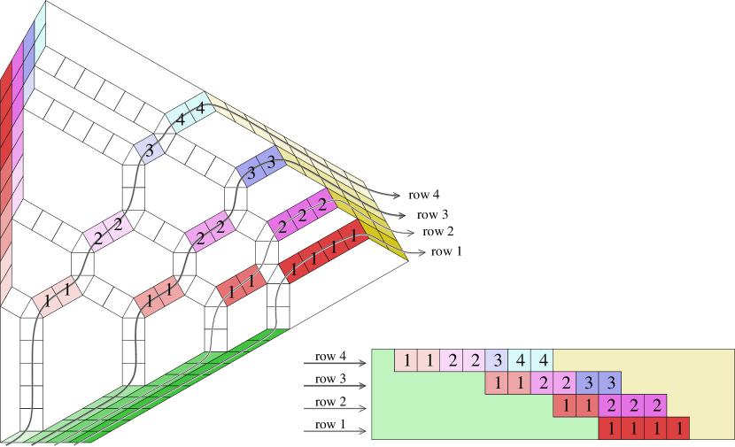
Figure 9: Bijection between mosaics and Littlewood-Richardson tableaux.

Proposition 5.1.

The following bijections between mosaics and Littlewood-Richardson tableaux coincide:

1. Tao’s bijection as formulated in Figure 9;

2. the bijection obtained by $\alpha$ orientation $(E_{A},N_{A})$ and migrating from $A$ to $B$ (second bijection in Table 1);

3. the bijection obtained by giving $\alpha$ orientation $(-E_{A},-N_{A})$ and migrating from $A$ to $C$.

This correspondence allows us to see the connection with jeu de taquin.

Proposition 5.2.

Under the bijection of Proposition 5.1 the migration of a single rhombus from $B$ to $C$ (or vice-versa) corresponds to a Schützenberger slide.

Corollary 5.3.

Under the bijection of Proposition 5.1, rotating a mosaic $120^{\circ}$ counterclockwise corresponds to the transformation $f\mapsto\tilde{g}$ of LR-tableaux described below.

1. Begin with an LR-tableau $f$ with boundary data $(\nu,\lambda^{\vee},\mu)$.

2. Replace each entry by its position in the reverse of the standard order and rotate this by $180^{\circ}$. The result will have shape $\mu^{\vee}/\lambda^{\vee}$. Call this tableau $\tilde{f}$.

3. Let $g$ be the unique straight LR-tableaux of shape $\lambda^{\vee}$.

4. Perform reverse jeu de taquin on $g$: slide the boxes of $\tilde{f}$, in order, through $g$, to produce a new tableau $\tilde{g}$ with boundary data $(\lambda^{\vee},\mu,\nu)$.

Proof.

By Proposition 5.2 the tableau $\tilde{g}$ is the result of migrating rhombi from $B$ to $C$ with the orientation $(E_{B},N_{B})$. ∎

Thus we see that any migration corresponds to some sequence of jeu de taquin operations, using Proposition 5.2 and Corollary 5.3. Hence, questions about migration can be translated into questions about jeu de taquin. We will not attempt to fully explore the consequences of this correspondence here, but since so much is already known about jeu de taquin, this is a powerful fact. For example, the following statement is not at all obvious from the results in Section 3, but can be shown using jeu de taquin methods.

Proposition 5.4.

Each of the bijections described in the proofs of Corollaries 3.3 and 3.4 is an involution.

5.2 Open questions

The reader may at first wonder whether the map $\lozenge\mapsto\lozenge^{\prime}$ is a picture in the sense of Zelevinsky. It is easily seen that this is not the case; however, since $(f,f^{\prime})$ is a pair of LR-tableaux of the same content, this pair corresponds to a picture, by Zelevinsky’s generalisation of the Robinson-Schensted-Knuth correspondence [Z]. Is there an easy way to describe this picture in terms of migration.

One aspect of this picture which is a bit perplexing is the number of choices available in making any of the constructions which prove commutativity and associativity. Even after one chooses orientations on the flocks, there is more than one way to move the flocks around inside a (bi)mosaic so that they end up in the correct final positions. Each of these different choices could conceivably give rise to different commutors and associators (i.e. bijections which prove commutativity and associativity). However, the fact that questions about these operations can be reformulated in terms of jeu de taquin limits the number of possibilities. It would be nice to be able to see that certain bijections were independent of choices without resorting to the fact that this is true for jeu de taquin.

One can consider the groupoid whose objects are (bi)mosaics with flocks, and whose arrows are sequences of migrations. What is this groupoid? Is there monodromy, i.e. when the flocks return to their original positions in their original orientations, do we necessarily get back to the same mosaic? It should be possible to answer this question using the correspondence with jeu de taquin, but again, it would be preferable to somehow get an answer directly.

Finally, puzzles, and therefore mosaics, have a geometric interpretation [V] in terms of degenerations of Richardson varieties. Can migration be understood in terms of this picture? If not, perhaps migration can be geometrically interpreted in a different way. If this is possible, it may be the nicest way to understand why certain operations are independent of choices, as well as answer the monodromy question.

References

- [BSS] G. Benkart, F. Sottile and J. Stroomer, Tableau Switching: Algorithms and Applications J. Comb Theory A. 76 (1996), no. 1, 11–43.
- [BKT] A. Buch, A. Kresch and H. Tamvakis, Littlewood-Richardson rules for Grassmannians, Adv. Math. 197 (2005), no. 1, 306–320.
- [F] W. Fulton, Young tableaux with applications to representation theory and geometry, Cambridge University Press, New York, 1997.
- [KT1] A. Knutson and T. Tao, The honeycomb model of tensor products I: proof of the saturation conjecture, J. Amer. Math. Soc. 12 (1999), no. 4, 1055–1090.
- [KT2] A. Knutson and T. Tao, Puzzles and (equivariant) cohomology of Grassmannians, Duke Math. J. 119 (2003), no. 2, 221–260.
- [KTW1] A. Knutson, T. Tao, and C. Woodward, The honeycomb model of tensor products II. Puzzles determine facets of the Littlewood-Richardson cone, J. Amer. Math. Soc. 17 (2004), no. 1, 19–48 (electronic).
- [KTW2] A. Knutson, T. Tao, and C. Woodward, A positive proof of the Littlewood-Richardson rule using the octahedron recurrence. Electron. J. Combin. 11 (2004), Research Paper 61, 18 pp.
- [LR] D.E. Littlewood and A.R. Richardson, Group characters and algebra, Philos. Trans. Roy. Soc. London. 233 (1934), 99–141.
- [S] M.-P. Schützenberger, La correspondance de Robinson. Combinatoire et représentation du groupe symétrique, pp. 59–113. Lecture Notes in Math., Vol. 579, Springer, Berlin, 1977.
- [V] R. Vakil, A geometric Littlewood-Richardson rule, to appear in Ann. Math. (preprint math.AG/0302294, 2003)
- [Z] A. V. Zelevinsky, A generalization of the Littlewood-Richardson rule and the Robinson-Schensted-Knuth correspondence, J. Algebra 69 (1981), no. 1, 82–94.