Force distributions and force chains in random stiff fiber networks

Abstract

We study the elasticity of random stiff fiber networks. The elastic response of the fibers is characterized by a central force stretching stiffness as well as a bending stiffness that acts transverse to the fiber contour. Previous studies have shown that this model displays an anomalous elastic regime where the stretching mode is fully frozen out and the elastic energy is completely dominated by the bending mode. We demonstrate by simulations and scaling arguments that, in contrast to the bending dominated elastic energy, the equally important elastic forces are to a large extent stretching dominated. By characterizing these forces on microscopic, mesoscopic and macroscopic scales we find two mechanisms of how forces are transmitted in the network. While forces smaller than a threshold $F_{c}$ are effectively balanced by a homogeneous background medium, forces larger than $F_{c}$ are found to be heterogeneously distributed throughout the sample, giving rise to highly localized force-chains known from granular media.

1 Introduction

It has been well known for more than a century that networks of central force springs lose their rigidity when the number of connected neighbours is lower than a certain threshold value maxwell1864 . To guarantee the rigidity of these otherwise “floppy” networks, additional contributions to the elastic energy, beyond central-force stretching, have to be introduced sahimi . Here our focus is on a particular class of heterogeneous networks composed of crosslinked fibers, whose length $l_{f}$ is much larger than the typical distance $l_{s}$ between two fiber-fiber intersections (see Fig. 1). These systems have recently been suggested as model systems for studying the mechanical properties of paper sheets alava06 or biological networks of semiflexible polymers frey98 ; bausch06 ; heu06a . As only two fibers may intersect at a given cross-link, the average number of neighboring cross-links is $z<4$. This places them below the rigidity transition both in two and in three spatial dimensions. Several strategies have been used to elastically stabilize a central-force fiber network lat01springs . Here, we use an additional energy cost for fiber “bending”. The bending mode penalizes deformations transverse to the contour of the fiber while to linear order the distance between cross-links, i.e. the length of the fiber, remains unchanged.

The two-dimensional fiber network we consider is defined by randomly placing $N$ initially straight elastic fibers of length $l_{f}$ on a plane of area $A=L^{2}$ such that both position and orientation are uniformly distributed. The fiber density is thus defined as $\rho=Nl_{f}/A$. We consider the fiber-fiber intersections to be perfectly rigid, but freely rotatable cross-links that do not allow for relative sliding of the fibers. The elastic building blocks of the network are the fiber segments, which connect two neighbouring cross-links. A segment of length $l_{s}$ is modeled as a classical beam with cross-section radius $r$ and bending rigidity $\kappa$ landau7 . Loaded along its axis (central force “stretching”) such a slender rod has a rather high stiffness, characterized by the spring constant $k_{\parallel}(l_{s})\sim\kappa/l_{s}r^{2}$, while it is much softer with respect to transverse deformations $k_{\perp}(l_{s})\sim\kappa/l_{s}^{3}$ (“bending”).

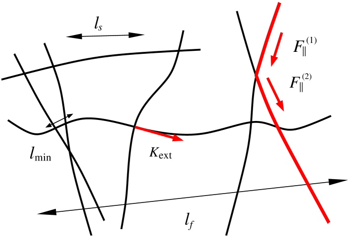
Figure 1: Illustration of the local network structure and the relevant length-scales in the random fiber network (drawn in the deformed configuration): the fiber length $l_{f}$, the typical segment length $l_{s}$ and the shortest deformed segment of length $l_{\rm min}$. $K_{\rm ext}$ signifies the bending force that the crossing fiber exerts in the axial direction of the horizontal fiber. $F_{\parallel}^{(1)}$ and $F_{\parallel}^{(2)}$ correspond to axial forces that are directly transmitted from one fiber to a neighboring fiber at the crosslink. This mechanism forms the basis for the establishment of force-chains; see main text.

While this random fiber network is known to have a rigidity percolation transition at a density $\rho_{c}$ lat01 ; wil03 ; hea03b , we have recently shown heu06floppy ; heu07condmat how the network’s inherent fragility, induced by its low connectivity $z$, determines the properties even in the high-density regime far away from the percolation threshold, $\rho\gg\rho_{c}$. In particular, it was possible to explain the anomalous scaling properties of the shear modulus as found in simulations wil03 ; hea03a . The unusually strong density dependence of the elastic shear modulus $G\sim(\rho-\rho_{c})^{6.67}$ wil03 is found to be a consequence of the architecture of the network that features various different length-scales heu06floppy ; heu07condmat (see Fig. 1). On the mesoscopic scale the fiber length $l_{f}$ induces a highly non-affine deformation field, where segment deformations $\delta_{\rm na}$ follow the macroscopic strain $\gamma$ as $\delta_{\rm na}\sim\gamma l_{f}$. This is in stark contrast to an affine deformation field where deformations scale with the size of the object under consideration. For a segment of length $l_{s}$ the affine deformation therefore is $\delta_{rmaff}\propto\gamma l_{s}$. Microscopically, a second length $l_{\min}$ governs the coupling of a fiber segment to its neighbours on the crossing fiber heu06floppy ; heu07condmat . Due to the fact that the bending stiffness $k_{\perp}\sim l_{s}^{-3}$ of a segment is strongly increasing with shortening its length, it is found that segments with $l_{s}<l_{\rm min}$ rather deform their neighbours than being deformed, while longer segments $l_{s}>l_{\rm min}$ are not stiff enough to induce deformations in the surrounding. Thus $l_{\rm min}$ plays the role of a rigidity scale, below which segments are stiff enough to remain undeformed. As a consequence the elastic properties of the fiber as a whole are not governed by the average segment $\bar{l}_{s}$, but rather by the smallest loaded segment $l_{\min}$.

In the observed scaling regime the elastic modulus does originate exclusively in the bending of the individual fibers, and thus reflects the stabilising effect of this soft deformation mode. In contrast, stretching deformations in this non-affine bending dominated regime can be assumed to be frozen out completely. In our previous articles heu06floppy ; heu07condmat we have dealt with the properties of the bending mode, $k_{\perp}$, and its implications on the elastic energy. Here we focus on the stretching mode, $k_{\parallel}$, and its role in the occurence of elastic forces. As the non-affine bending regime is relevant for slender fibers with a small cross-section radius, $r\to 0$, it is characterized by a scale separation, $k_{\parallel}/k_{\perp}\sim r^{-2}\to\infty$, which assures that no stretching deformations, $\delta_{\parallel}$, occur. Thus, the fibers effectively behave as if they were inextensible bars. Closer inspection of the limiting process reveals, however, that the stretching deformations tend to zero as $\delta_{\parallel}\sim 1/k_{\parallel}$ . This makes the contribution to the total energy $W_{s}\sim k_{\parallel}\delta_{\parallel}^{2}\sim k_{\parallel}^{-1}$ negligible, as required, but also implies that finite stretching forces $F_{\parallel}$ will occur,

$$F_{\parallel}\sim k_{\parallel}\delta_{\parallel}\to\rm const\,.$$ (1)

Indeed, these forces, acting axially along the backbone of the fibers, are absolutely necessary to satisfy force-balance at the intersection of two fibers. With two fibers intersecting at a finite angle it is intuitively clear that a change in transverse force in one fiber has to be balanced by an axial force in the second.

For thicker fibers with a larger cross-section radius $r$, a second elastic regime occurs, where the bending instead of the stretching mode is frozen out. This regime formally corresponds to the limit $k_{\parallel}/k_{\perp}\sim r^{-2}\to 0$. It is characterized by stretching deformations of mainly affine character hea03a . The elastic shear modulus (as well as the Young’s modulus) have been shown to depend linearly on density wil03 ; ast00 ; ast94 , $G\sim\rho$, which is in striking contrast to the strong susceptiblity to density variations found in the non-affine bending regime.

In the following we will present results of simulations that characterize in detail the occuring axial forces in both elastic regimes, the non- affine bending as well as the affine stretching regime. In the simulations we subject the network to a macroscopic deformation and determine the new equilibrium configuration by minimizing the elastic energy. The minimization procedure is performed with the commercially available finite element solver MSC.MARC. Further details of the simulation procedure can be found in our previous publications heu06a . Starting with the average force-profile along the fibers we then proceed by giving the full probability distribution of forces. We show that its tails are heterogeneously distributed throughout the system, similar to force-chains in granular media. We find that most of the features can be understood with the help of the two basic length-scales, the filament length $l_{f}$ and the rigidity scale $l_{\min}$.

2 Effective Medium Theory

In this section we will characterize the configurationally averaged force profile along a fiber. In the spirit of an effective medium theory, one can think of the fiber as being imbedded in an elastic matrix that, on a coarse-grained scale, acts continuously along the backbone. The associated force ${\cal K}_{\rm ext}$, which is imposed on the fiber, leads to a change in axial force according to landau7

$$\frac{\partial F_{\parallel}}{\partial s}=-{\cal K}_{\rm ext}\,,$$ (2)

where $s$ is the arclength along the fiber backbone.

A while back, Cox cox51 provided a second, constitutive equation that allows to solve for the force profile $F_{\parallel}(s)$. He assumed the medium to be characterized by an affine deformation field $\delta_{\rm aff}(s)\sim\gamma s$. The external force ${\cal K}_{\rm ext}$ is assumed to be non- vanishing only when the actual fiber deformation $\delta_{\parallel}$ is different from this affine deformation field,

$${\cal K}_{\rm ext}(s)=k\left(\delta_{\parallel}-\delta_{\rm aff}(s)\right)\,.$$ (3)

Eqs. (2) and (3) can easily be solved and result in a force profile that shows a plateau in the center of the fiber as well as boundary layers where the force decreases exponentially, $F_{\parallel}(s)=a-b\cosh[c(s-l_{f}/2)]$, with $a$, $b$, and $c$ appropriately chosen constants.

Åström et al. ast94 have applied this model to the affine stretching regime and found the boundary layers to grow as the fiber cross-section radius is decreased. Fig. 2 shows results of our simulations for the force profile both in the affine stretching regime (blue squares) and the non-affine bending regime (red circles). Apparently the Cox-model accounts very well for the force profile in the stretching regime, while it fails completely in the bending regime, where the simulation data clearly show that the force increases linearly from the boundary towards the center of the fiber.

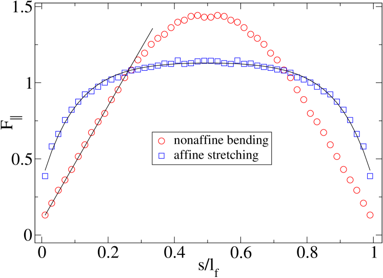
Figure 2: Variation of average axial force $F_{\parallel}$ along the backbone $s=[0,l_{f}]$ of the fibers (symmetrized around $s=l_{f}/2$). The symbols are the results of our simulations. Towards the fiber ends the force relaxes exponentially in the affine stretching regime (full curve is a fit to the Cox model), and linearly in the non-affine bending regime.

Cox ideas can be generalized to the non-affine bending regime, where the elastic medium entirely consists of bending modes. In this regime the axial forces in the fiber arise due to the pulling and pushing of its crossing neighbors that try to transfer their high bending load in a kind of lever-arm effect (see Fig.1). As explained above, the deformation field is non-affine and, instead of $\delta_{\rm aff}$, one has to use $\delta_{\rm na}\sim\gamma l_{f}$ heu07condmat , which is proportional to the fiber length $l_{f}$. Since we are interested in the limit where stretching deformations vanish, $\delta_{\parallel}\to 0$, the resulting exernal force is arclength independent, ${\cal K}_{\rm ext}=-k\delta_{\rm na}\sim-l_{f}$ and constant along the backbone. The axial force profile $F_{\parallel}(s)$ is thus expected to be linearly increasing from the boundaries towards the center, in agreement with the simulations.

Recently, Head et al. hea03a have suggested growing boundary layers to play a key role for the cross-over from the affine stretching to the non-affine bending regime. Here, we have shown that these growing boundary layers are rather a consequence of a transition from an exponential to a linear force profile in the boundary layers. This follows naturally from the fact that non-affine deformations, $\delta_{\rm na}$, scale with the fiber length $l_{f}$ and not with the segment length $l_{s}$. As we have analyzed in detail in Ref. heu07condmat , this scaling property, which originates in the network architecture, can be understood within a “floppy mode” concept. Therefore, the growing boundary layers should be viewed as a consequence rather than the driving force of the affine to non-affine transition.

3 Force distribution

We now turn to a discussion of the full probability distribution of axial forces, instead of just the average value as we have done in the previous section. In Fig. 3 we display the distribution function $P(F_{\parallel})$ for various densities $\rho$ deep in the non-affine regime. Remarkably, the curves for different densities collapse on a single master curve by using the scaling ansatz

$$P(F_{\parallel})=F_{c}^{-1}h(F_{\parallel}/F_{c})\,,$$ (4)

with the force scale $F_{c}=\kappa\rho_{c}^{2}(\delta\!\rho/\rho_{c})^{5}$, where $\delta\!\rho=\rho-\rho_{c}$.

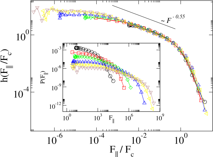
Figure 3: Probability distribution $P(F_{\parallel})$ (inset) and scaling function $h$ in the non-affine bending regime with aspect ratio $r/l_{f}=5\cdot 10^{-6}$ for various densities $\rho l_{f}=20...100$. The force scale used to obtain the data collapse is $F_{c}=\kappa\rho_{c}^{2}(\delta\!\rho/\rho_{c})^{5}$.

Its appearance in Eq. (4) indicates that $F_{c}$ is the average axial force. We now show that it is furthermore equivalent to the average bending force $F_{c}=\langle k_{\perp}(l_{s})\cdot\delta_{\rm na}\rangle$ that is needed to impose the non-affine bending deformation $\delta_{\rm na}$ on a segment of bending stiffness $k_{\perp}$.

The average $\langle.\rangle$ is performed over the segment-length distribution $P(l_{s})$ , restricted to those segments that are longer than the rigidity scale $l_{\rm min}$. Recall, that $l_{\rm min}$ plays the role of the shortest deformed segment such that shorter segments do not contribute to the averaging. The equivalence of both expressions for the force scale becomes evident by writing the average explicitly,

$$F_{c}=\int_{l_{\rm min}}^{\infty}\!dl_{s}P(l_{s})k_{\perp}(l_{s})\delta_{\rm na}\,,$$ (5)

and inserting $k_{\perp}\sim l_{s}^{-3}$. The integral is dominated by its lower limit, which leads to $F_{c}\sim\kappa(\rho l_{f})^{5}/l_{f}^{2}$ as required.

Hence, the force scale $F_{c}$ has been identified as the average force that induces the non-affine bending of a fiber. At the same time it occurs in the probability distribution of stretching forces as depicted in Fig. 3. This two-fold role reflects the interplay of bending and stretching in the effective medium theory, where stretching forces in one fiber have to be balanced by bending forces in its neighbors. We can thus conclude that the effective medium picture is the appropriate description for forces up to the threshold $F_{c}$, i.e. for the “typical” properties of the system.

Interestingly, for forces smaller than $F_{c}$ the probability distribution displays an intermediate power-law tail $h(x)\sim x^{-\beta}$, with an exponent $\beta\approx 0.55$, which as yet defies a simple explanation. For forces larger than $F_{c}$, one may even speculate about the existence of a second power-law regime with a much higher exponent $\beta^{\prime}\approx 5$. While in this regime the distribution does not seem to decrease exponentially, the available range of forces is too small to reach any final conclusions as to the functional form.

The axial forces in the affine stretching regime follow a completely different probability distribution, as can be seen from Fig. 4.

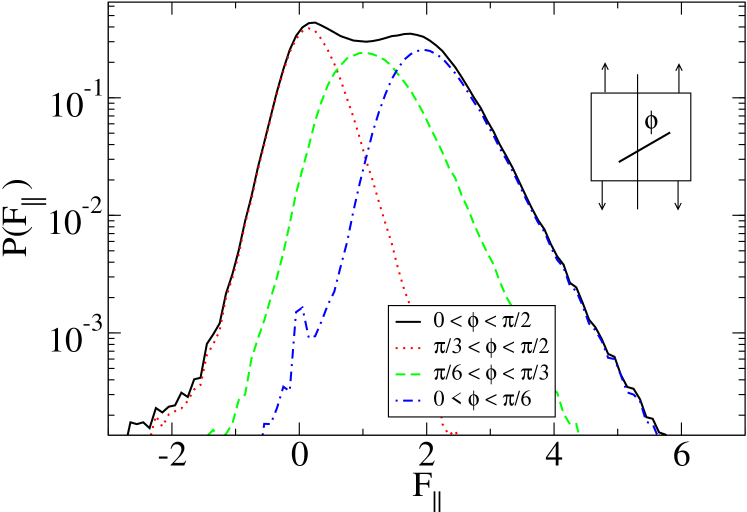
Figure 4: Probability distribution $P(F_{\parallel})$ of axial forces in the affine stretching dominated regime for $\rho l_{f}=60$ and aspect ratio $r/l_{f}=0.05$. The system is subject to uniaxial stretching, as indicated in the inset. Note the linear scale on the $x$-axis. The peak of the distribution is strongly correlated with the orientation, $\phi$, of the fiber relative to the principal stretching direction.

The solid black line relates to the probability distribution of all segments, irrespective of their orientation $\phi$, with respect to the imposed strain field (in this case: uniaxial extension along the $y$-direction). The broken lines only include segments with orientations $\phi$ in a particular interval, as denoted in the figure legend. The tails of the distribution are exponential (as has previously been observed in Ref. ast94 ), while the peak force strongly depends on the orientation $\phi$ of the segments. The position of the peak follows naturally from the assumption that segments undergo affine deformations with $\delta_{\rm aff}=\gamma l_{s}\cos^{2}\phi$. Since the resulting affine forces $F_{\rm aff}(\phi)=k_{\parallel}(l_{s})\delta_{\rm aff}\sim\kappa\gamma\cos^{2}\phi$ do not depend on the length of the segments, one expects only a single, orientation-dependent force, that is a delta-function distribution $P(F,\phi)\sim\delta(F-F_{\rm aff}(\phi))$. The broadening of the distribution relative to the singular delta-function can be rationalized with the fact that the affine strain field can only fulfill force equilibrium if the fibers are infinitely long. For finite fibers the force has to drop to zero at the ends (as discussed above), leading to additional (non-affine) deformations and therefore to a broadening of the peak.

4 Force-chains

In the preceding two sections we have characterized the occuring axial forces on the scale $l_{f}$ of a single fiber as well as on the smaller scale of an indivdual fiber segment $l_{s}$. We now proceed to discuss the properties of the forces on a larger, mesoscopic scale. To this end we probe the Green’s function of the system and impose a localized perturbation in the center of the network. Fixing the boundaries, we displace a single crosslink and monitor the resulting response of the network. Similar studies have been conducted in Ref. hea05 , where ensemble averaging is used to discuss the applicability of homogeneous elasticity theory. Here, we focus on the individual network realization to better characterize the spatial organization of the forces.

In Figs. 5 and 6 we show pictures of a network, where the grey-scales of the segments are chosen according to the magnitude of the forces they carry. The higher the force the darker the segment. While the quenched random structure is the same in both plots, the fiber aspect ratio $\alpha=r/l_{f}$ is chosen such that the network lies deep in the non-affine bending ($\alpha=10^{-5}$) or the affine stretching regime ($\alpha=10^{-1}$), respectively. As is clearly visible in Fig. 5 the non-affine response is characterized by well defined paths of high forces that extend from the center, where the force is applied, to the boundaries. These forces are transmitted from fiber to fiber along a zig-zag course. Upon comparison with the distribution function for axial forces (like those shown in Fig. 3), we find that the force-chains are constituted by forces with magnitude larger than $F_{c}$ (i.e. above the intermediate power-law regime). In contrast, in the affine regime a rather homogeneous distribution of forces is observed (Fig. 6).

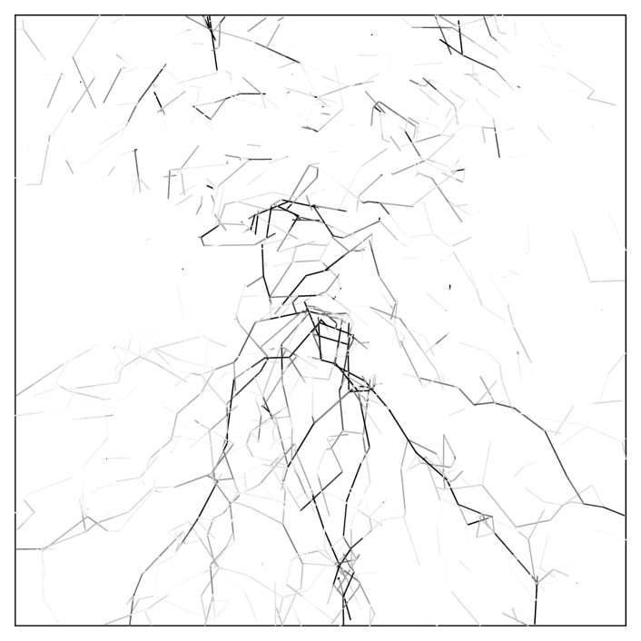
Figure 5: Picture of a network in the non-affine bending dominated regime. The grey-scale is chosen according to the axial force in the segment. Force-chains are clearly visible, and follow a zig-zag course from the center towards the lower boundary.

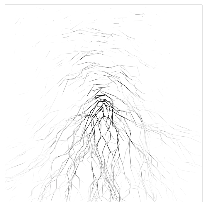
Figure 6: Picture of a network in the affine stretching dominated regime. The grey-scale is chosen according to the axial force in the segment. No force-chains are present.

The observation that the highest occuring forces are connected in chains, suggests a mechanism that allows direct transmission of an axial load from one fiber to the next. This has to be contrasted with the results of Sec. 2, where we have developed an effective medium picture that constitutes an indirect load transfer, in which axial forces in one fiber are balanced by transverse (bending) forces in the neighboring fiber. The difference between both mechanisms becomes evident by considering the load transfer at a fiber-fiber intersection that coincides with the end-point of one of the two fibers; see Fig. 7 for an illustration. An axial load $F_{\parallel}^{(1)}$ that is coupled into fiber $(1)$ at its left end has to be taken up by the crossing fiber $(2)$ at the distal end of fiber $(1)$. Assume that this applied force in the horizontal fiber, $F_{\parallel}^{(1)}$, is accompanied with an axial displacement $\delta\!z_{1}$, which translates the fiber along its axis.

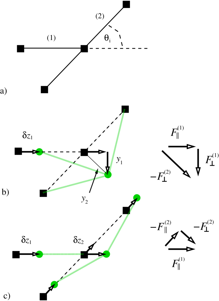
Figure 7: Illustration of the two mechanisms of load transfer for a fiber segment (1) ending at a crossing fiber (2). The displacement $\delta\!z_{1}$ of the horizontal fiber leads to deformations in both fibers. The indirect load transfer, b), couples axial forces into bending deformations, while the direct transfer, c), transmits the axial force directly into axial forces in the neighboring fiber.

In the indirect load transfer the axial force $F_{\parallel}^{(1)}$ is balanced by bending forces $F_{\perp}^{(1,2)}$ oriented perpendicular to the contour of both fibers. The force balance reads

$$F_{\parallel}^{(1)}+F_{\perp}^{(1)}=-F_{\perp}^{(2)}\,.$$ (6)

The angle between both fibers being $\theta$, the associated bending displacements are (Fig. 7b)

$$y_{1}=-\delta\!z\cot\theta\,,\quad y_{2}=\delta\!z/\sin\theta\,.$$ (7)

This mechanism forms the basis of the effective medium theory applied in Sec. 2 to explain the average force profile along the fibers. It has also been shown to allow a direct calculation of the macroscopic elastic moduli of the network heu06floppy ; heu07condmat .

We now proceed to discuss the second mechanism. It can immmediately be seen from the $\theta$-dependence that the bending displacements $y_{1/2}$ of Eq.(7) can become increasingly large, if the fibers intersect at small enough angles, $\theta\to 0$. Then, the network responds in a different way. As can be inferred from Fig. 7c the large bending contributions may be avoided by additionally moving the secondary fiber along its own axial direction, $\delta\!z_{2}=\delta\!z_{1}\cos\theta$. This leaves the primary fiber straight while the bending displacement in the secondary fiber becomes $y_{2}=\delta\!z_{1}\sin\theta$. The force balance must therefore be written as

$$F_{\parallel}^{(1)}=-(F_{\parallel}^{(2)}+F_{\perp}^{(2)})\,.$$ (8)

The smaller the angle $\theta$ the larger is the contribution of $F_{\parallel}^{(2)}$, which is just the forward “scattering” of forces, seen in Fig. 5.

The existence of force-chains is intimately connected to the presence of long fibers, $\rho l_{f}\gg 1$. Since the coordination can be written as $z=z_{c}(1-O(\rho l_{f})^{-1})$ heu07condmat , the system will become completely rigid by increasing the fiber length, $l_{f}\to\infty$. There, the force scale $F_{c}$ diverges and axial forces imposed on a fiber will propagate along the fiber completely uncorrelated with forces on its neighbours. As the number of intersections $n_{\rm cl}\sim\rho l_{f}$ per fiber is proportional to the fiber length, the probability distribution for the angle between two intersecting fibers is sampled to an increasing degree. In particular, the smallest angle that will occur in a finite sample of $n_{cl}$ intersections is calculated from

$$\int_{0}^{\theta_{\min}}d\theta P(\theta)=1/n_{cl}\,,$$ (9)

as $\theta_{\min}\sim l_{f}^{-1/2}$, where we have used $P(\theta)\sim\theta$ for small values of $\theta$. With increasing fiber length ever smaller angles occur. As explained above, the presence of small angles necessarily lead to forward scattering of axial forces, and thus to the emergence of force-chains. The presence of force-chains is therefore a consequence of the special geometry of the network that allows the fibers to intersect at arbitrarily small angles. To support this view, we have conducted additional simulations in which the localized perturbation is applied in varying directions. As a result, the structure of the force-chains remain unchanged while their amplitudes are modulated.

5 Conclusion and Outlook

In conclusion, we have characterized in detail the properties of forces occuring in two-dimensional random fiber networks. We have shown that the previously identified rigidity scale $l_{\min}$, in addition to the structural scale of the fiber length $l_{f}$, governs the occurence of stretching forces in an elastic regime, where the energy derives from the bending mode only ($k_{\parallel}/k_{\perp}\to\infty$). The probability distribution of forces shows scaling behaviour with the force scale $F_{c}=\kappa\rho_{c}^{2}(\delta\!\rho/\rho_{c})^{5}$ that can be identified with the average force needed to deform a fiber segment by the non-affine deformation $\delta_{\rm na}\sim\gamma l_{f}$.

Two types of force transmission have been identified. Forces up to the scale $F_{c}$ are transmitted from one fiber to the next by an indirect mechanism, where stretching forces are balanced by bending forces and vice versa. This is best illustrated by the action of a lever-arm that tries to transmit its bending load to the neighboring fiber, which subsequently starts to stretch (see ${\cal K}_{\rm ext}$ in Fig.1). This mechanism of force transmission can be used to understand the average force profile along a fiber, and also forms the basis for the calculation of the scaling properties of the elastic modulus heu06floppy ; heu07condmat . In a second direct mechanism axial forces are also transmitted directly to their neighbors, giving rise to highly localized force-chains that are heterogeneously distributed throughout the sample. This mechanism is only active for forces larger than $F_{c}$. In contrast to the indirect mechanism, which probes the center of the force distribution and therefore typical properties of the network, the direct mechanism reflects the properties of the extremal values of the distribution.

The observation of force-chains suggests an analogy with granular media JaegerRMP96 . The scale separation $k_{\parallel}\gg k_{\perp}$ implies that the fibers behave as if they were inextensible. The network of inextensible segments may therefore loosely be viewed as the contact network of a system of rigid grains. Due to the low coordination number, the fiber network has to be stabilised by the action of the bending mode directed perpendicularly to the fiber axis. This bears some similarity to a friction force in granular systems, which is directed tangentially to the grain surfaces. Indeed, it has been argued that stable granular systems with a coordination as low as found here may only be achieved if frictional forces are taken into account unger05 . The occurence of force chains in our “frictional” system is, however, due to the vicinity of the isostatic point with regard to the frictionless system ($z_{c}=4$). Since the coordination may be written as $z=4(1-O(\rho l_{f})^{-1})$ the isostatic point is reached by increasing the fiber length $l_{f}\to\infty$.

We gratefully acknowldege fruitful discussions with Klaus Kroy. Financial support of the German Science Foundation (SFB486) and of the German Excellence Initiative via the program ”Nanosystems Initiative Munich (NIM)” is gratefully acknowledged.

References

- (1) J. C. Maxwell, Philos. Mag. 27, (1864) 27.
- (2) M. Sahimi, Heterogeneous Materials (Springer, New York, 2003).
- (3) M. Alava and K. Niskanen, Rep. Prog. Phys. 69, (2006) 669.
- (4) E. Frey, K. Kroy, J. Wilhelm, and E. Sackmann, in Dynamical Networks in Physics and Biology, edited by G. Forgacs and D. Beysens (Springer, Berlin, 1998), Chap. 9.
- (5) A. Bausch and K. Kroy, Nature Physics 2, (2006) 231.
- (6) C. Heussinger and E. Frey, Phys. Rev. Lett. 96, (2006) 017802, Phys. Rev. E 75, (2007) 011917.
- (7) M. Latva-Kokko, J. Mäkinen, and J. Timonen, Phys. Rev. E. 63, (2001) 046113.
- (8) M. Latva-Kokko and J. Timonen, Phys. Rev. E 64, (2001) 066117.
- (9) J. Wilhelm and E. Frey, Phys. Rev. Lett. 91, (2003) 108103.
- (10) D. A. Head, A. J. Levine, and F. C. MacKintosh, Phys. Rev. E 68, (2003) 25101.
- (11) C. Heussinger and E. Frey, Phys. Rev. Lett. 97, (2006) 105501.
- (12) C. Heussinger, B. Schaefer, and E. Frey, cond-mat/0703095.
- (13) D. A. Head, A. J. Levine, and F. C. MacKintosh, Phys. Rev. Lett. 91, (2003) 108102, Phys. Rev. E 68, (2003) 61907.
- (14) J. A. Åström, S. Saarinen, K. Niskanen, and J. Kurkijä rvi, J. Appl. Phys. 75, (1994) 2383.
- (15) J. A. Åström, J. P. Mäkinen, M. J. Alava, and J. Timonen, Phys. Rev. E 61, (2000) 5550.
- (16) L. D. Landau and E. M. Lifshitz, Theory of Elasticity, 3rd ed. (Butterworth-Heinemann, Oxford, 1995), Vol. 7.
- (17) H. L. Cox, Br. J. Appl. Ph. 3, (1951) 72.
- (18) D. A. Head, A. J. Levine, and F. C. MacKintosh, Phys. Rev. E 72, (2005) 061914.
- (19) H. M. Jaeger, and S. R. Nagel, Rev. Mod. Phys. 68, (1996) 1259.
- (20) T. Unger, J. Kertész, and D. E. Wolf, Phys. Rev. Lett. 94, (2005) 178001.