Dynamics of light propagation in spatiotemporal dielectric structures

Abstract

Propagation, transmission and reflection properties of linearly polarized plane waves and arbitrarily short electromagnetic pulses in one-dimensional dispersionless dielectric media possessing an arbitrary space-time dependence of the refractive index are studied by using a two-component, highly symmetric version of Maxwell’s equations. The use of any slow varying amplitude approximation is avoided. Transfer matrices of sharp nonstationary interfaces are calculated explicitly, together with the amplitudes of all secondary waves produced in the scattering. Time-varying multilayer structures and spatiotemporal lenses in various configurations are investigated analytically and numerically in a unified approach. Several new effects are reported, such as pulse compression, broadening and spectral manipulation of pulses by a spatiotemporal lens, and the closure of the forbidden frequency gaps with the subsequent opening of wavenumber bandgaps in a generalized Bragg reflector.

1 Introduction

Propagation of electromagnetic waves through stationary inhomogeneous media is a subject that has been extensively studied in the past [1, 2].

The physics of moving dielectric media [3, 4, 5, 6, 7] is attracting renewed attention, mainly due to recent works by Visser [8] and Leonhardt and Piwnicki [9]. Particularly important is the formal equivalence between the equations of general relativity and the equations of light propagation in arbitrarily moving dielectric media, which has been fully recognized in the early literature [10].

Much less attention, however, has been devoted to the case of light propagation through an inhomogeneous medium which possesses a time-dependent refractive index, and in particular light scattering by nonstationary interfaces between two media with different refractive indices. This must be distinguished from the above case of a moving medium, in that the nonstationary interfaces may possess arbitrary velocity $v$, in the range $0<|v|<\infty$. This well-known fact [11] is not in conflict with special relativity because the medium itself is immobile, and only the interfaces of the transition regions of the refractive index change in time. This apparent motion of the interfaces is due to the time-varying nature of the refractive index, since it is not connected to the real motion of any physical particle or wave, and is not restricted by any limiting velocity, so that the function $n(z,t)$ that describes the spatiotemporal variations of the refractive index is completely arbitrary. In particular Lorentz transformations, which of course play a crucial role in the physics of moving media, are not applicable to the physics of media with a time-varying refractive index. For example, the field amplitudes of the waves generated inside the latter media are not found via Lorentz boosts, and the constitutive relations between the dielectric displacement and the electric field are fixed and not subject to Lorentz transformations, in contrast with the physics of moving media, described, for instance, in Refs. [3, 4].

The first attempt to develop a theory for the very special case of plane wave propagation in a homogeneous medium with a sudden step-like temporal variation of refractive index has been given by Morgenthaler in 1958 [12], but only after more than a decade this work has been noticed and other aspects of propagation in the same system have been explored by Felsen and Whitman in 1970 [13] and by Fante in 1971 [14]. A more recent review of the salient features of the optics of nonstationary media, with particular emphasis on plasma physics applications, has been given by Shvartsburg in 2005 [15].

The purpose of the present paper is to study the effect of an arbitrary space- and time-dependence of refractive index $n(z,t)$ on the propagation of electromagnetic waves and pulses in media without dispersion. We shall provide a unified theoretical approach, with which we are able to study the scattering of light by nonstationary interfaces moving at arbitrary velocities. Light propagation through media with a small number of nonstationary interfaces has been investigated by a variety of experimental techniques [19, 20, 21, 22, 23, 24], as discussed further in the final discussion and conclusions section. Our results here include these cases but also address the behavior that could be achieved by further extension to an arbitrary number of well-controlled nonstationary interfaces. Our aim is to demonstrate the potential of nonstationary dielectrics for light control and manipulation.

The paper is organized as follows.

In Section 2 we construct the basic theoretical tools that are necessary for the analysis and the understanding of the building blocks of spatiotemporal dielectric structures. First of all, in subsection 2.1 our master equation [Eq.(2)] is derived from Maxwell’s equations, and its geometrical interpretation in terms of forward- and backward-moving fields is given. After that, in subsection 2.2 the interface transfer matrix for the general case is calculated explicitly, while in subsection 2.3 the expression for free propagation when the fields are far from interfaces is derived, and a criterion for defining sharp interfaces is found. In subsection 2.4 we use special orthogonal variables to introduce plane wave expansion of arbitrary fields, which allows us to find the transfer propagation matrix in Fourier space.

In Section 3 we describe three fundamental applications of the concept expressed in Section 2. In subsection 3.1 the reflection and transmission coefficients of several important configurations of nonstationary interfaces are derived, and numerical simulations of pulse scattering from interfaces are provided in order to confirm the theoretical expressions. In subsection 3.2 we discuss nonstationary multilayer structures, and provide the analogue of quarter wavelength condition for a generalized nonstationary Bragg reflector, and the transformation of the bandstructure and the bandgaps under rotations of the $(z,ct)$-plane are examined. In subsection 3.3 we deal with a special device, the spatiotemporal analogue of a lens. We show, including numerical simulations, how such a lens can be used to perform pulse compression or broadening, with the consequent manipulation of pulse frequency and wavenumber.

The results presented in Sections 2 and 3 are obtained by solving the full Maxwell equations. We derive in Section 4 an exact equation to describe the evolution of the pulse envelope. We consider how this equation is modified if we introduce a slowly varying envelope approximation (SVEA) in time. Numerical simulations are then presented to show that the SVEA introduces errors in the detail of pulse propagation for the problems we are considering, due to the neglect of effects associated with sharp spatiotemporal interfaces. Finally we summarize our conclusions in Section 5.

2 Analytical Results

2.1 Main Equation

Let us start by assuming that we have an electromagnetic wave, with its electric and magnetic fields $\mathbf{E}=[E(z,t),0,0]^{T}$ and $\mathbf{B}=[0,B(z,t),0]^{T}$ linearly polarized along the directions $\hat{x}$ and $\hat{y}$ respectively. The $x$-component of the electric field and the $y$-component of the magnetic field depend on the variable $z$ only, because in conditions of normal incidence we assume that any change of the time-dependent refractive index occurs along the propagation direction $\hat{z}$. The linear polarization $\mathbf{P}_{L}$ of the medium will be written in the form $\mathbf{P}_{L}=\chi(z,t)\mathbf{E}=[n(z,t)^{2}-1]\mathbf{E}$, where $\chi$ is the linear susceptibility of the non-magnetic medium and $n(z,t)$ is the linear space-time dependent refractive index, which is assumed for simplicity to be independent of the frequency $\omega$ and to be real. This model for the susceptibility is obviously simplified, but for the purposes of the present paper the frequency dispersion of the refractive index is not essential and will be disregarded for sake of clarity. Here and in the following we choose to use the very convenient Heaviside-Lorentz units system [3], in which $\mathbf{E}$, $\mathbf{B}$ and $\mathbf{P}_{L}$ are measured in the same physical units (V/m), and there are no extra multiplying factors $4\pi$, $\epsilon_{0}$ and $\mu_{0}$ in Maxwell’s equations. Maxwell’s equations for the scalar quantities $E(z,t)$ and $B(z,t)$ can be written in the following form ($c$ is the speed of light in vacuum):

$$\partial_{t}(n^{2}E)+c\partial_{z}B=0,\qquad\partial_{t}B+c\partial_{z}E=0,$$ (1)

where the two divergence Maxwell’s equations are automatically satisfied due to the chosen polarization and the normal incidence assumption.

It is possible to cast Eqs.(1) in a different form, which turns out to be much more convenient for the analysis of time-varying photonic crystals and lenses, using the fact that the problem under consideration is (1+1)-dimensional. Defining local right- and left-moving fields, $F^{\pm}\equiv(nE\pm B)/2$, we can write Eqs.(1) in the following compact form:

$$\left[\hat{\partial}+\sigma_{x}(\hat{\partial}\ln{n})\sigma_{x}^{+}\right]\Psi=0,$$ (2)

where $\Psi\equiv[F^{+},F^{-}]^{T}$ (with the superscript $T$ we indicate vector transposition), and

$$\sigma_{0}=\left(\begin{array}[]{cc}1&0\\ 0&1\end{array}\right),\qquad\sigma_{x}=\left(\begin{array}[]{cc}0&1\\ 1&0\end{array}\right)\qquad\sigma_{z}=\left(\begin{array}[]{cc}1&0\\ 0&-1\end{array}\right),$$ (3)

are the identity matrix and the first and third (real) Pauli matrices. Moreover, $\sigma^{\pm}_{j}\equiv(\sigma_{0}\pm\sigma_{j})/2$ are the Pauli projectors ($j=\{x,z\}$), and $\hat{\partial}$ is the derivative operator

$$\hat{\partial}\equiv\frac{n}{c}\sigma_{0}\partial_{t}+\sigma_{z}\partial_{z}\equiv\left(\begin{array}[]{cc}\partial^{+}&0\\ 0&\partial^{-}\end{array}\right),$$ (4)

with $\partial^{\pm}\equiv(n/c)\partial_{t}\pm\partial_{z}$. $(\partial^{+},\partial^{-})$ can be thought of as basis vectors for a tangent space $\mathcal{TM}$ of the two-dimensional manifold $\mathcal{M}$ formed by the $(z,ct)$-plane equipped with a space-time dependent refractive index function $n(z,t)$ [16]. The spatiotemporal evolution of the dielectric structure is only contained in the logarithmic term $\hat{\partial}\ln{n}$, which couples the forward- and the backward-propagating components of the electromagnetic field. All conclusions of this paper are based on an analysis of the main Eq.(2).

One can appreciate the remarkably high level of symmetry between space and time contained in Eq.(2) with the following arguments. The propagation of the local field $F^{+}$ occurs only along the (local) direction specified by $\partial^{+}$, while the field $F^{-}$ evolves only along $\partial^{-}$. Therefore $\partial^{+}$ and $\partial^{-}$ determine, at each point of the $(z,ct)$-plane, the local light cone along which the forward and backward components of the electric field propagate. The geometrical meaning of our construction based on Eq.(2) is depicted in Fig. 1, where examples of the local light cones defined by the directions determined by $\partial^{\pm}$ and the propagating forward/backward fields $F^{\pm}$ are shown (see also caption for further explanation of the geometrical meaning of our construction).

Contrary to a widespread approach [17], we do not make use of any complex slowly varying variable, such as a field envelope, and therefore Eq.(2) remains valid for all regimes of propagation, and all quantities appearing in Eq.(2) are real. A slow variable version of Eq.(2) will be examined in Section 4, and a comparison between the exact approach of Eq.(2) and the approximate one of Eq.(45) will be presented.

Note that the coupling between $F^{+}$ and $F^{-}$ is only induced via the logarithmic term $\hat{\partial}\ln{n}$ in Eq.(2), so that only space-time variations of the refractive index are responsible for coupling forward and backward waves during propagation. We can therefore identify two basic cases in which the analytical solution of Eq.(2) is straightforward, namely the case where $n$ changes abruptly from $n_{1}$ to $n_{2}$ along a line in the $(z,ct)$-plane, and the case of a homogeneous and static medium, where Eq.(2) simply becomes $\hat{\partial}\Psi=0$. In the following two subsections these two cases are examined individually.

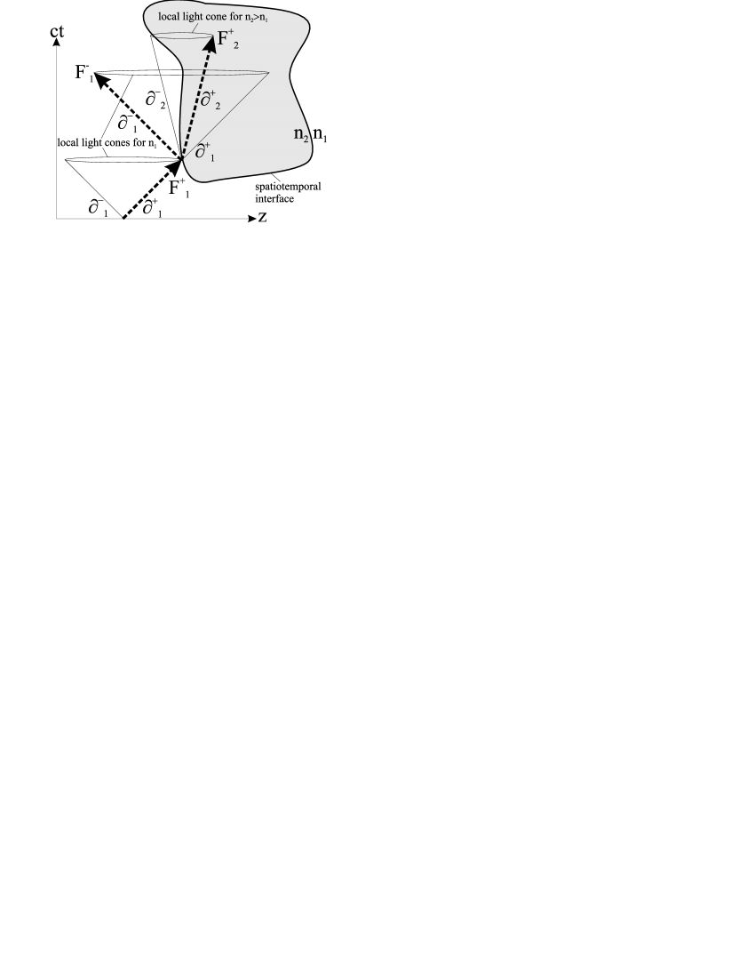
Figure 1: The geometry of propagation of fields $F^{\pm}_{j}$ along the directions determined by $\partial^{\pm}_{j}$ is shown, where $j=\{1,2\}$ refers to the refractive index $n_{j}$. The grey area represents the spatiotemporal region of refractive index change in the plane $(z,ct)$. For this simple example, the external and the internal regions have uniform indices $n_{1}$ and $n_{2}$ respectively. Bold dashed arrows indicate the propagating fields, generated by the scattering of $F^{+}_{1}$ from an interaction point on the interface. Local light cones are also indicated. Assuming that $n_{2}>n_{1}$, wider light cones are associated with index $n_{1}$, whereas narrower light cones are associated with index $n_{2}$. Only space-time variations of refractive index are able to generate coupling between forward and backward waves in Eq.(2), so that in the case shown in the figure only the interface is able to scatter an incident electromagnetic wave.

2.2 Calculation of the Interface Matrix

We assume that the refractive index changes in a step-like fashion along a nonstationary interface in the $(z,ct)$-plane, postponing the discussion of the validity of this sharpness assumption to the end of the next paragraph. The generic form of the refractive index is then given by $n(z,t)=n_{1}+(n_{2}-n_{1})\Theta(\cos(\theta)z-\sin(\theta)ct)$, where $n_{1,2}$ are the refractive indices of the first and the second media, and $\Theta$ is the Heaviside function. $\theta$ denotes the angle between the $ct$-axis and the interface in the $(z,ct)$-plane, which we will occasionally also parameterize via the slope parameter $\beta=\tan(\theta)$. Note that the quantity $\beta c$ represents the velocity of the nonstationary interface. This velocity is arbitrary, and in particular it can be greater than the local speed of light. This is not in conflict with special relativity, because the nonstationary interface is not associated with a moving medium, and it constitutes one of the main differences between the present work and previous literature on nonstationary dielectrics. For different aspects of the physics of moving media the reader is referred to chapter IX of Landau [4], section I.5 of Jackson [3], and to more recent works by Yeh and collaborators [5], Saca [6], Huang [7] and by Leonhardt and Piwnicki [9].

Our task is now to find an appropriate transfer matrix connecting the amplitudes of the fields $F^{\pm}$ on either side of the interface. We call this an interface matrix. Using the appropriate orthogonal coordinates

$$p(z,t) = \cos(\theta)z-\sin(\theta)ct=\frac{z-\beta ct}{\sqrt{1+\beta^{2}}},$$ (5)

$$q(z,t) = \sin(\theta)z+\cos(\theta)ct=\frac{\beta z+ct}{\sqrt{1+\beta^{2}}},$$ (6)

normal ($p$) and parallel ($q$) to the interface in the $(z,ct)$-plane, we can express the derivative operator in Eq.(2) as $\hat{\partial}=\hat{A}\partial_{p}+\hat{B}\partial_{q}$, with the matrices $\hat{A}$ and $\hat{B}$ defined as

$$\hat{A} \equiv [\sigma_{z}\cos(\theta)-n\sigma_{0}\sin(\theta)]$$ (7)

$$\hat{B} \equiv [\sigma_{z}\sin(\theta)+n\sigma_{0}\cos(\theta)].$$

Taking into account that $\partial_{q}n=0$ we can write Eq.(2) in the form

$$\left[\partial_{p}+\hat{A}^{-1}\hat{B}\partial_{q}+\hat{A}^{-1}\sigma_{x}\hat{A}(\partial_{p}\ln{n})\sigma_{x}^{+}\right]\Psi=0.$$ (8)

Writing Eq.8 in the basis $[nE,B]^{T}=(\sigma_{x}+\sigma_{z})\Psi$ yields the following set of ordinary differential equations:

$$\partial_{p}\left(\ln nE\right)+\frac{1}{n^{2}\beta^{2}-1}\left[-\beta\left(1+n^{2}\right)\partial_{q}(\ln nE)\right.$$ (9)

$$\left.-n\left(1+\beta^{2}\right)\frac{\partial_{q}B}{\left(nE\right)}+\left(1+n^{2}\beta^{2}\right)\left(\partial_{p}n\right)\right] = 0,$$

$$\partial_{p}(B)+\frac{1}{n^{2}\beta^{2}-1}\left[-\beta\left(1+n^{2}\right)\partial_{q}(B)\right.$$ (10)

$$\left.-n\left(1+\beta^{2}\right)\partial_{q}\left(nE\right)+2n\beta\left(\partial_{p}n\right)\left(nE\right)\right] = 0.$$

We can now integrate Eq. (9) from $p=-\epsilon$ to $p=+\epsilon$ across the interface at $p=0$, where $\epsilon$ is an arbitrarily small positive number. If $B$ and $(nE)$ are differentiable with respect to $q$ (i.e. $\partial_{q}B<\infty$ and $\partial_{q}\ln nE<\infty$), and additionally $n^{2}\beta^{2}\neq 1$ across the interface, then the contributions to this integral from terms containing $\partial_{q}(B)$ and $\partial_{q}\left(nE\right)$ are proportional to $\epsilon$ and will therefore vanish in the limit $\epsilon\to 0$; Eq. (9) can then be integrated analytically. Under the same conditions Eq. (10) can also be integrated analytically and we obtain a linear relation between $[n_{1}E_{1},B_{1}]^{T}$ and $[n_{2}E_{2},B_{2}]^{T}$. In the $[F^{+},F^{-}]^{T}$ basis this relation can be expressed via the interface matrix $D^{[12]}$ for the step-like transition that connects the fields $F^{\pm}$ in medium 1 with those in medium 2:

$$\left(\begin{array}[]{c}F^{+}_{1}\\ F^{-}_{1}\end{array}\right)=D^{[12]}\left(\begin{array}[]{c}F^{+}_{2}\\ F^{-}_{2}\end{array}\right).$$ (11)

Explicitly we find

$$D^{[12]}=\frac{1}{2n_{2}}\left(\begin{array}[]{cc}(n_{1}+n_{2})\frac{1-n_{2}\beta}{1-n_{1}\beta},&(n_{1}-n_{2})\frac{1+n_{2}\beta}{1-n_{1}\beta}\\ (n_{1}-n_{2})\frac{1-n_{2}\beta}{1+n_{1}\beta},&(n_{1}+n_{2})\frac{1+n_{2}\beta}{1+n_{1}\beta}\end{array}\right).$$ (12)

This interface matrix possesses the classical property $(D^{[12]})^{-1}=D^{[21]}$. For future reference it is also useful to calculate

$$\det D^{[12]}=\left(\frac{1-n_{2}^{2}\beta^{2}}{1-n_{1}^{2}\beta^{2}}\right)\frac{n_{1}}{n_{2}}.$$ (13)

Note that in the derivation of 12 we have used that $n^{2}\beta^{2}\neq 1$ as we cross the interface. In particular this implies that our derivation is not valid in the regime where $1/n_{2}<|\beta|<1/n_{1}$. The physical reason for this will be discussed at the end of the next subsection, after we introduce the free propagation matrix.

2.3 Free Propagation in Real Space

From the knowledge of the general transfer matrix for a nonstationary interface [Eq.(12)], it is possible to construct the transfer matrix for more complicated nonstationary objects, such as multilayer structures, which will be done in Section 3. However, we still need to construct one missing ingredient, the so-called propagation matrix, which models the propagation of the fields along the $p$-direction far from the interfaces, where the refractive index is constant. Under this condition, Eq.(2) simply becomes $\hat{\partial}\Psi=0$, which using the definitions of Eq. 7 can be expressed as

$$\hat{A}\partial_{p}\Psi+\hat{B}\partial_{q}\Psi=0.$$ (14)

To solve Eq.(14), we first write the derivatives $\partial_{p,q}$ as first order finite differences, namely $\partial_{p}\Psi=[\Psi(p+\Delta p,q)-\Psi(p,q)]/\Delta p$ and $\partial_{q}\Psi=[\Psi(p,q+\Delta q)-\Psi(p,q)]/\Delta q$, and then substitute into the equation:

$$\hat{A}\frac{\Psi(p+\Delta p,q)-\Psi(p,q)}{\Delta p}+\hat{B}\frac{\Psi(p,q+\Delta q)-\Psi(p,q)}{\Delta q}=0.$$ (15)

For a fixed $\Delta p$, we can eliminate the term proportional to $\Psi(p,q)$ in Eq.(15) with an appropriate choice of $\Delta q$, different for the two components of the $\Psi$-vector. From Eqs.7 one obtains

$$\Delta q^{\pm}=\frac{\sin(\theta)\pm n\cos(\theta)}{\cos(\theta)\mp n\sin(\theta)}\Delta p,$$ (16)

where the refractive index $n$ refers to the homogeneous layer under consideration, and $\Delta q^{\pm}$ refers to the component $F^{\pm}$. With the particular choice of Eq.(16), the free propagation of the optical fields for constant refractive index assumes a particularly simple and effective form, which we write for the two components:

$$F^{\pm}(p+\Delta p,q)=F^{\pm}(p,q+\Delta q^{\pm}).$$ (17)

This means that advancing the field $F^{\pm}$ along the $p$-direction by a small step $\Delta p$ (keeping $q$ constant), is equivalent to advancing the same field by an amount equal to $\Delta q^{\pm}$ along the $q$-direction (keeping $p$ constant). The geometrical interpretation of Eq.(17) is that the points $(p+\Delta p,q)$ and $(p,q+\Delta q^{\pm})$ belong to the same light cone.

The concept of the interface matrix [Eq.(12)] expressed in Section 2.2 is only valid for a sufficiently sharp interface, i.e. if the interface transition layer is sufficiently thin, such that the effect of the propagator (17) can be neglected while traversing the interface. For a given interface width $\Delta p$ we can calculate via (16) the length of the interval $\Delta q^{\pm}$ along the interface which is relevant for the propagator. If $F^{\pm}$ does not change significantly on this interval, i.e. if

$$\Big{|}\partial_{q}\ln F^{\pm}\frac{\beta\pm n}{1\mp n\beta}\Delta p\Big{|}\ll 1,$$ (18)

then the propagator is negligible and the use of the interface matrix of Eq.(12) is justified. Note however that the left hand side of Eq.18 becomes singular for $n\beta=\pm 1$, and then 18 will not be fulfilled for any choice of $\Delta p$. In particular, for $n_{2}>n_{1}$, if $1/n_{2}<\beta<1/n_{1}$, then during the integration of 8 we will reach the point where the singularity in 18 occurs. This is precisely at the point where the matrix $\hat{A}^{-1}$ also becomes singular. The condition on the sharpness of the interface which was used in the derivation of Eq.(12) can therefore in principle not be fulfilled and therefore we shall not use Eq.(12) in the regime of $1/n_{2}<\beta<1/n_{1}$.

2.4 Plane wave expansion. Calculation of Propagation Matrix

So far we have expressed the interface matrix of Eq.(12) and the free propagator of Eq.(17) as operating on the fields vector $\Psi(p,q)$, where $p$ and $q$ are the rotated variables of Eqs. (5) and (6). However, the interface matrix of Eq.(12) connects the fields $F^{+}$ and $F^{-}$ only along the $p$-direction, while not affecting the fields along the $q$-direction at all. It is therefore natural to consider a plane wave expansion along the $q$-axis,

$$\Psi(p,q)=\sum_{\tilde{\omega}}\Psi^{\tilde{\omega}}(p)e^{-i\tilde{\omega}q}.$$ (19)

Then Eq.(11) transforms into

$$\Psi^{\tilde{\omega}}_{1}=D^{[12]}\Psi^{\tilde{\omega}}_{2},$$ (20)

which means that the generalized frequency $\tilde{\omega}$ is conserved across the interface. $\tilde{\omega}$ has the dimension of a wavenumber, and physically it represents the momentum associated to the propagation along the $q$-direction.

Inside a homogeneous medium we can expand $\Psi(p,q)$ in plane waves along both the $p$ and $q$ axes:

$$\Psi(p,q)=\sum_{\tilde{\omega},\tilde{k}}\Psi^{\tilde{\omega},\tilde{k}}e^{i(\tilde{k}p-\tilde{\omega}q).}$$ (21)

Since each plane wave component has to fulfill the propagator equation $\hat{\partial}\Psi^{\tilde{\omega},\tilde{k}}e^{i(\tilde{k}p-\tilde{\omega}q)}=0$, we obtain for the two components $F^{\pm}$ the following dispersion relations:

$$\tilde{k}^{\pm}=\frac{\sin(\theta)\pm n\cos(\theta)}{\cos(\theta)\mp n\sin(\theta)}\tilde{\omega},$$ (22)

which can also be directly deduced from Eq.(16). This enables us to rewrite the free propagator (17) for the Fourier components as

$$\Psi^{\tilde{\omega}}(p+\Delta p)=P(\Delta p)\Psi^{\tilde{\omega}}(p)=\left(\begin{array}[]{cc}e^{i\tilde{k}^{+}\Delta p}&0\\ 0&e^{i\tilde{k}^{-}\Delta p}\end{array}\right)\Psi^{\tilde{\omega}}(p),$$ (23)

an expression that will be useful in Section 3.2.

As a final issue, it is worth writing explicitly the transformation law between the momenta ($\tilde{k}$,$\tilde{\omega}$), reciprocal to the real-space variables $(p,q)$ respectively, and $(k,\omega)$, reciprocal to the variables $(z,ct)$. By using Eqs.(5)-(6) and the expansion of Eq.(21) we obtain:

$$\left(\begin{array}[]{c}\tilde{k}\\ \tilde{\omega}\end{array}\right)=\left(\begin{array}[]{cc}\cos(\theta)&\sin(\theta)\\ -\sin(\theta)&\cos(\theta)\end{array}\right)\left(\begin{array}[]{c}k\\ \omega/c\end{array}\right).$$ (24)

From the simple rotation of Eq.(24) one can deduce some important physical consequences. First of all for $\theta=0$ ($\beta=0$) it follows that $\tilde{k}=k$ and $\tilde{\omega}=\omega/c$, so that in the static case the $p$-direction coincides with the $z$-axis and the $q$-direction coincides with the $ct$-axis by definition. But because the $q$-direction is associated with the delocalization direction of an arbitrary plane wave in Eq.(21), it follows that during the scattering process of light by a static interface the quantity $\tilde{\omega}=\omega/c$ is conserved. This corresponds to the energy conservation at the interaction point. In other words, all generated waves will have exactly the same frequency. The other limiting case is when $\theta\rightarrow\pi/2$ ($\beta\rightarrow\infty$). For this case the role of frequency and wavenumber is reversed, and from Eq.(24) we have $\tilde{k}=\omega/c$ and $\tilde{\omega}=-k$. The delocalization direction is still along $q$, which now points along the $z$-axis. Therefore during the scattering it is the wavenumber (i.e. the momentum) that is conserved at the interaction point, and in general all generated waves will have different frequencies but the same momentum. For an intermediate situation ($0<\theta<\pi/2$), the conserved quantity $\tilde{\omega}$ corresponds to a combination of $k$ and $\omega/c$ according to the rotation of Eq.(24).

3 Applications

In the present section we discuss three fundamental applications of the concepts expressed in Section 2.2, and in particular of the transfer interface matrix given by Eq.(12) and the free propagator given in real space by Eq.(17) and in Fourier space by Eq.(23).

In subsection 3.1 we analyze the physics of scattering by nonstationary interfaces in different interesting physical configurations, shown in Fig. 2. In subsection 3.2 we calculate the bandstructure and the forbidden bandgaps of a nonstationary photonic crystal, finding a novel effect: the closure of the frequency bandgap for a certain value of $\theta=\theta_{cr1}$, and the consequent opening of the wavenumber bandgap for another $\theta=\theta_{cr2}$. In subsection 3.3 we show that it is possible to think of a dynamical device, analogous to a spatiotemporal lens, that efficiently performs pulse broadening and compression, with simultaneous frequency/wavenumber manipulation of pulses.

3.1 Nonstationary interfaces

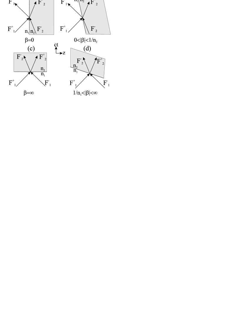
Figure 2: Panel showing space-time diagrams of scattering of forward and backward fields $F^{\pm}_{j}$ ($j=\{1,2\}$) from the four most important interface configurations. (a) Space-like interface ($\beta=0$, $\theta=0$), which coincides with the conventional, static interface. (b) Interface configuration with $\beta<0$ and $0<|\beta|<1/n_{2}$. (c) Time-like interface, $\beta=\pm\infty$ ($\theta=\pm\pi/2$). (d) Interface configuration with $\beta<0$ and $1/n_{1}<|\beta|<\infty$.

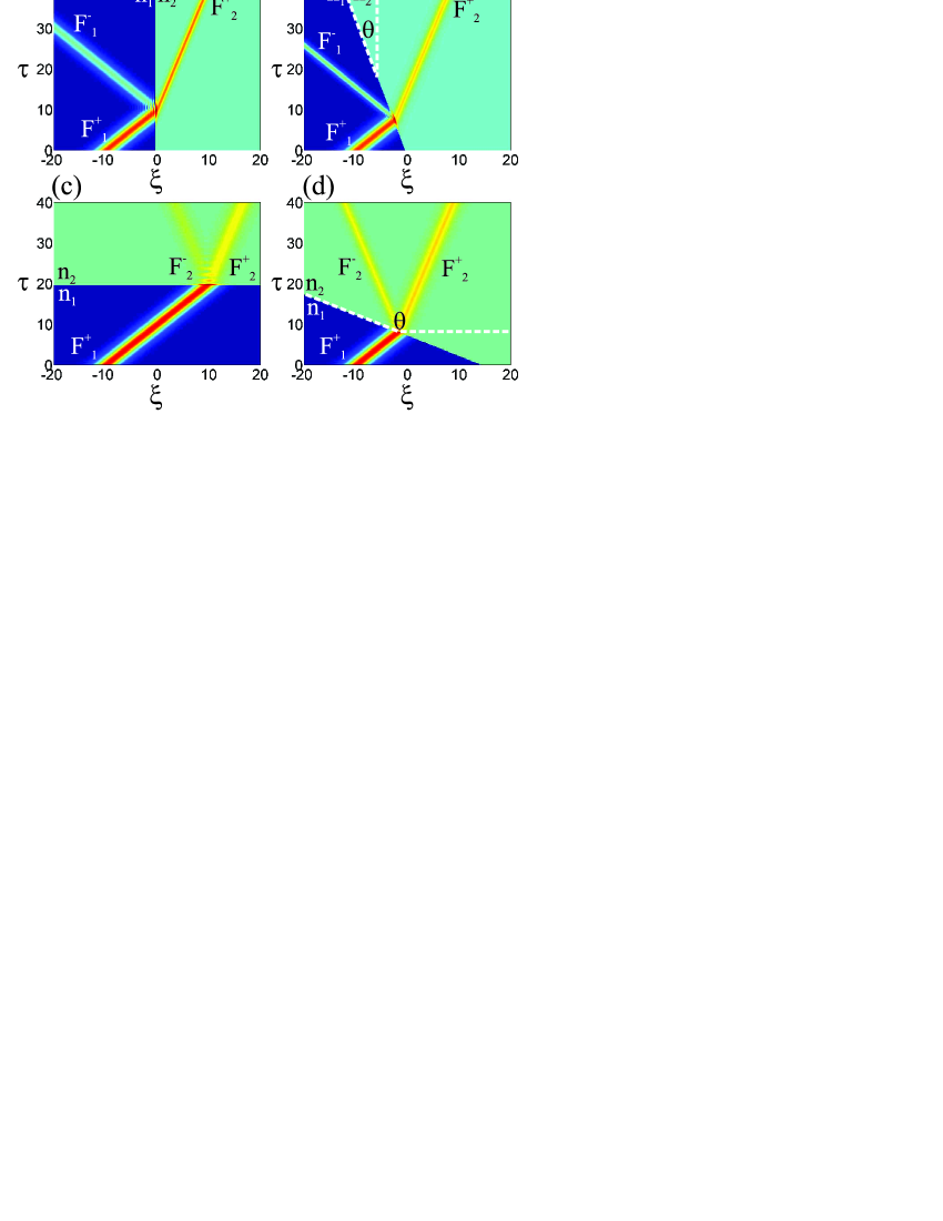
Figure 3: (Color online) Panel showing the simulation of interaction of an incoming pulse with the four sharp interface configurations of Fig. 2. (a) Space-like interface: $\beta=0$. (b) $\beta=-0.3$. Angle $\theta=-0.2915$ radians is indicated with dashed lines. (c) Time-like interface: $\beta=\infty$. (d) $\beta=-2$. Angle $\theta=-1.1071$ radians is indicated with dashed lines. Refractive indices are: $n_{1}=1$ and $n_{2}=3$. The agreement with theoretical expressions is excellent for all cases. Input pulse parameter $w$ in Eq.(33) is $w=1$. Horizontal axis is dimensionless space coordinate $\xi=z/\lambda$, while the vertical axis is dimensionless time coordinate $\tau=ct/\lambda$, and $\lambda$ is the central pulse wavelength.

The panel of Fig. 2 shows the four most important cases of interface configurations which can be analyzed with the help of Eq.(12). Let us first consider Fig. 2(a) which shows the space-time diagram of a conventional static interface ($\theta=0$, $\beta=0$) between two media of refractive indices $n_{1}$ and $n_{2}$ respectively in the plane $(z,ct)$. Because all the variation of the refractive index is spatial, and the variable $p$ defined in Eq. (5) can be identified with the spatial coordinate $z$, we call this a space-like interface. By taking the limit $\beta\rightarrow 0$ in Eq.(12) we find the well-known result for the interface matrix:

$$D^{[12]}_{\beta=0}=\frac{1}{2n_{2}}\left(\begin{array}[]{cc}n_{1}+n_{2},&n_{1}-n_{2}\\ n_{1}-n_{2},&n_{1}+n_{2}\end{array}\right).$$ (25)

The transmission and reflection coefficients are then classically defined for $F_{2}^{-}=0$ as

$$t \equiv \frac{F^{+}_{2}}{F_{1}^{+}}=\frac{1}{D^{[12]}_{11}}=\frac{2n_{2}}{n_{1}+n_{2}},$$ (26)

$$r \equiv \frac{F^{-}_{1}}{F_{1}^{+}}=\frac{D^{[12]}_{21}}{D^{[12]}_{11}}=\frac{n_{1}-n_{2}}{n_{1}+n_{2}}.$$ (27)

For $0<|\beta|<1/n_{2}$ as in Fig. 2(b) the configuration is similar to the one in Fig. 2(a). From the interface matrix Eq.(12) we can now calculate the generalized transmission and reflection coefficients according to the definitions of Eqs.(26)-(27) as

$$t=\frac{2n_{2}}{n_{1}+n_{2}}\frac{1-n_{1}\beta}{1-n_{2}\beta},\quad r=\frac{n_{1}-n_{2}}{n_{1}+n_{2}}\frac{1-n_{1}\beta}{1+n_{1}\beta}.$$ (28)

Note that for $\beta<0$ and inside the parameter region $0<|\beta|<1/n_{2}$, the expressions given by Eq.(28) never show any singularity in the denominator. However, for $\beta>0$, we have a singularity in the transmission coefficient for $\beta\rightarrow 1/n_{2}$. This limit corresponds to the disappearance from the equations of one of the waves participating in the scattering ($F^{+}_{2}$), which will travel exactly along the interface, so that $t$ as given by Eq.(28) cannot be used, and for $\beta>1/n_{2}$ the incident light never reaches the interface.

For $|\beta|=\infty$ Fig. 2(c) shows the configuration when the refractive index changes abruptly and simultaneously in time throughout all space (for some discussion of the experimental relevance of this concept see the conclusions, Section 5). Because the variation of the refractive index occurs only along the $ct$-axis, we shall call this a time-like interface. From Eq. (12) we obtain the interface matrix

$$D^{[12]}_{\beta=\infty}=\frac{1}{2n_{1}}\left(\begin{array}[]{cc}n_{1}+n_{2},&n_{2}-n_{1}\\ n_{2}-n_{1},&n_{1}+n_{2}\end{array}\right).$$ (29)

For the calculation of the transmission and reflection coefficients we have now to set $F_{1}^{-}=0$, and then instead of Eqs. (26) and (27) we obtain

$$t \equiv \frac{F^{+}_{2}}{F_{1}^{+}}=D^{[21]}_{11}=\frac{n_{1}+n_{2}}{2n_{2}},$$ (30)

$$r \equiv \frac{F^{-}_{2}}{F_{1}^{+}}=D^{[21]}_{21}=\frac{n_{1}-n_{2}}{2n_{2}}.$$ (31)

Similar formulas for this special case have been given by Morgenthaler in 1958 [12]. For a more general $|\beta|>1/n_{1}$ when the interface is tilted with respect to the time-like case, the configuration is depicted in Fig. 2(d). Then Eqs. (30) and (31) generalize to

$$t=\frac{1-\beta n_{1}}{1-\beta n_{2}}\frac{n_{1}+n_{2}}{2n_{1}},\quad r=\frac{1-\beta n_{1}}{1+\beta n_{2}}\frac{n_{2}-n_{1}}{2n_{1}}.$$ (32)

Even in this case, the expressions of $t$ and $r$ in Eq.(32) have singularities for $\beta=1/n_{2}$ and $\beta=-1/n_{2}$ respectively, which however are outside the region of validity of these formulas, that is $|\beta|>1/n_{1}$.

In Section 2.4 we have seen that the frequency $\tilde{\omega}$ arising in the plane wave expansion along $q$ in Eq.(20) is conserved across the interface. As we have already discussed previously, in the case of $\beta=0$ [Fig. 2(a)] this is, with $\tilde{\omega}=\omega/c$, the well-know frequency (i.e. energy) conservation at a spatial interface. In the more interesting case $\beta=\infty$ [Fig. 2(c)], however, we see that $\tilde{\omega}=-k$, which means that wavenumber (i.e. momentum) is conserved at a time-like interface.

The scattering of finite pulses from the interfaces for all four cases shown in Fig. 2 have been simulated by solving numerically Eq.(2), and results are shown in the panel of Fig. 3. Electric field for the input pulse is taken of the form

$$E_{ini}\equiv E(z,t=0)=E_{0}\ \textrm{sech}\left(\frac{z}{w\lambda}\right)\cos\left(\frac{2\pi z}{\lambda}\right),$$ (33)

where $E_{0}$ is the incident amplitude, and $w$ is a dimensionless parameter which measures the spatial width in units of $\lambda$, the pulse central wavelength. Without loss of generality, the incident amplitude is in all cases normalized to the value $E_{0}=1$.

We have used a second order finite difference algorithm to model the derivatives in Eq.(2) for the two components, and a fourth order Runge-Kutta algorithm to advance the field in time. Once the spatial distribution of the electric field over the $z$-axis at the initial instant of time $E_{ini}=E(z,t=0)$ is given, the initial magnetic field $B_{ini}=B(z,t=0)$ can be found by imposing that there is no backward wave propagating for $t=0$, i.e. $F^{-}=0$, obtaining $B_{ini}(z)=n(z,t=0)E_{ini}(z)$, where $n(z,t=0)$ is the initial refractive index distribution. We use Neumann-type boundary conditions, which means that we impose that the derivatives of the optical fields vanish at the boundaries of the spatial window, while the evolution of the fields is calculated by advancing in time. In order to ensure complete stability of the numerical algorithm it is sufficient to impose that all fields are spatially localized and that the temporal step of the grid $\Delta t$ and the spatial step of the grid $\Delta z$ satisfy the following condition: $\Delta t\ll\Delta z^{2}$. For our simulations we always use a spatial sampling of the optical fields with a number of points equal to $N=2^{15}$, which is more than sufficient in order to obtain extremely accurate results for long propagation times, and to avoid the dangers of artifacts due to numerical dispersion during the temporal evolution.

The panel of Fig. 3 shows propagation of the envelope of the electric field (with the fast oscillations decoupled for sake of clarity) during the scattering processes analogous to Figs. 2(a,b,c,d) respectively. Here and in the following, contour plots are given in the dimensionless variables $\tau=ct/\lambda$ and $\xi=z/\lambda$, with $\lambda=2\pi c/\omega_{0}$, and $\omega_{0}$ is the central circular frequency of the initial pulse. Note that Eq.(2) is solved directly in dimensionless units, therefore we do not need to specify the scaling wavelength $\lambda$, and results shown in the figures can be adapted to the particular spatial scale that one chooses to consider. The extension of the spatial grid used is $\xi_{window}=300$ in dimensionless units, which is relatively large in order to ensure total spatial localization of all waves participating in the scattering, although only a small portion of this window is shown in the figures. The spatiotemporal steps are $\Delta\xi=9.15\times 10^{-3}$ and $\Delta\tau=7.67\times 10^{-7}$. The pulse is initially propagating at the speed of light in vacuum ($n_{1}=1$). The sharp interface is modeled through a Heaviside function $n(z,t)=n_{1}+(n_{2}-n_{1})\Theta(z-\beta ct)$, with $n_{2}=3$. The values of $\beta$ for Fig. 2(a,b,c,d) are respectively $\beta=0$, $\beta=-0.3$, $\beta=\infty$, and $\beta=-2$. In all cases, $t$ and $r$ as given by the theoretical analysis given above are predicted with a high degree of accuracy.

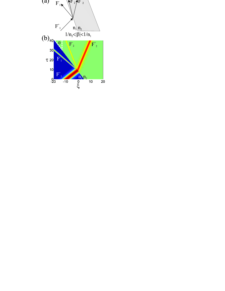
Figure 4: (Color online) (a) Scattering diagram in the case $\beta<0$, $1/n_{2}<|\beta|<1/n_{1}$, and (b) corresponding numerical simulation. Parameters are: $\beta=-0.4$ ($\theta=-0.3805$ radians, indicated with dashed lines), $w=1$. Refractive indices are: $n_{1}=1$ and $n_{2}=3$.

As discussed at the end of Section 2.3, the derivation of the interface matrix (12) does not cover the case of $1/n_{2}<|\beta|<1/n_{1}$. The configuration for this case is depicted in the upper panel of Fig. 4. We see that this case resembles the space-like configuration as in Fig. 2(a) in the region $n=n_{1}$ and the time-like configuration as in Fig. 2(c) for $n=n_{2}$. Note that now only one of the four fields ($F_{1}^{+}$) reaches the interaction point from the past, while the other three fields propagate from the interface in positive time direction. It is therefore not clear how in this case the transmission or reflection coefficient can be consistently defined, and neither of the given definitions of Eqs. (26)-(27) nor Eqs. (30)-(31) are satisfactory in this case. The theoretical origin of this problem is that in the region $1/n_{2}<|\beta|<1/n_{1}$ the transfer matrix concept is not applicable, due to the fact that for these values of $\beta$ the concept of sharp interface cannot be defined, at least using a dispersionless susceptibility, which does not make distinctions between long and short wavelengths. In particular, the condition of Eq.(18) does not necessarily hold in the above region, as recognized by Ostrovsky [11]. Nevertheless we can still solve Eq.(2) numerically as shown in Fig. 4(b), and we leave the investigation of this complicated issue for a future publication.

3.2 Nonstationary Photonic Crystals and Bandgap Calculation. Spatiotemporal Bragg reflector

We now use the knowledge built in Section 2.4 to calculate the bandstructure and the forbidden bandgaps of a nonstationary multilayer structure for different values of $\beta$, and in particular we shall enunciate the Bragg condition for a generalized Bragg reflector.

Let us assume in the following analysis that the periodicity of the multilayer structure is along the $p$-direction [see Fig. 5(a) and caption for a description of the geometry of the problem under consideration]. As in Section 2.4 we now deal with the propagation of plane waves of the form $\Psi(p,q)=\Psi^{\tilde{\omega}}(p)e^{-i\tilde{\omega}q}$. Similarly to the extensively studied Kronig-Penney model [18], we now look for a matrix $T$ such that

$$\Psi^{\tilde{\omega}}(p+\Lambda_{p})=T\Psi^{\tilde{\omega}}(p)$$ (34)

which propagates $\Psi^{\tilde{\omega}}(p)$ from the center of a layer with refractive index $n_{1}$ across a layer with refractive index $n_{2}$ into the center of the next layer with refractive index $n_{1}$ as indicated in Fig. 5(a). The length of this unit cell is given by $\Lambda_{p}=p_{1}+p_{2}$, where $p_{j}$ are the widths of the layers of indices $n_{j}$ along the $p$-direction. From Eqs. (20) and (23) we obtain

$$T=P_{1}(p_{1}/2)D^{[12]}P_{2}(p_{2})D^{[21]}P_{1}(p_{1}/2)$$ (35)

where $P_{j}(p)$ is the propagation matrix according to Eq.(23) in the medium with refractive index $n_{j}$. Since $D^{[12]}D^{[21]}=1$ we observe that $|\det T|=1$. Considering the two eigenvalues $\lambda_{1}^{T}$ and $\lambda_{2}^{T}$ of $T$ we can then distinguish between the following two cases: (i) $|\lambda_{1}^{T}|=|\lambda_{2}^{T}|=1$ and (ii) $|\lambda_{1}^{T}|>1$ and $|\lambda_{2}^{T}|<1$.

Free propagation will only occur in case (i), which by elementary algebra can be shown to be equivalent to

$$\frac{1}{2}|\textrm{Tr}\left(T\right)|<1.$$ (36)

In this case it is convenient to write the eigenvalues of $T$ in the form

$$\lambda_{1}=e^{i\bar{k}\Lambda_{p}}e^{i\tilde{K}\Lambda_{p}}\qquad\lambda_{2}=e^{i\bar{k}\Lambda_{p}}e^{-i\tilde{K}\Lambda_{p}},$$ (37)

where $\bar{k}$ is calculated via $\sqrt{\det T}=e^{i\bar{k}\Lambda_{p}}$ and $\tilde{K}$ fulfills the relation

$$\cos(\tilde{K}\Lambda_{p})=\frac{\textrm{Tr}\left(T\right)}{2\sqrt{\det T}}=\frac{\lambda_{1}+\lambda_{2}}{2e^{i\bar{k}\Lambda_{p}}}.$$ (38)

Physically $\bar{k}$ simply gives rise to a common phase factor in both eigenvalues of $T$, while $\tilde{K}$ can be interpreted as a generalization of the Bloch wavenumber in the Kronig-Penney model for nonstationary interfaces. In particular the explicit calculation of $\tilde{K}$ via a straightforward analytic expansion of the trace and determinant of $T$ yields the familiar-looking expression [18]:

$$\cos(\tilde{K}\Lambda_{p}) =\cos(p_{1}\tilde{k}^{\Delta}_{1})\cos(p_{2}\tilde{k}^{\Delta}_{2})$$

$$-\frac{n_{1}^{2}+n_{2}^{2}}{2n_{1}n_{2}}\sin(p_{1}\tilde{k}^{\Delta}_{1})\sin(p_{2}\tilde{k}^{\Delta}_{2}),$$

where

$$\tilde{k}^{\Delta}_{j}=\frac{\tilde{k}^{+}_{j}-\tilde{k}^{-}_{j}}{2}=\frac{n_{j}\tilde{\omega}}{\cos^{2}(\theta)-\sin^{2}(\theta)n_{j}^{2}}=\frac{(1+\beta^{2})n_{j}\tilde{\omega}}{1-\beta^{2}n_{j}^{2}.}$$ (40)

For a given $\tilde{\omega}$ we can now use Eqs. (3.2)-(40) to calculate the appropriate $\tilde{K}$, if it exists. This gives rise to a band structure relation as shown in Fig. 6 (see also caption). Note that $\beta$ only enters in the band structure calculation via $\tilde{k}^{\Delta}_{j}$, which however diverges for $\beta\rightarrow 1/n_{j}$ [cf. Eq. (40)].

The forbidden bandgaps are located in those regions of $\tilde{\omega}$ for which condition (36) is not fulfilled, i.e. the right hand side of Eq. (40) is larger than unity and $\tilde{K}$ would have a non-vanishing imaginary part, making the Bloch waves evanescent. In particular if the quantities $p_{j}$ are chosen such that

$$p_{j}\tilde{k}_{j}^{\Delta}=\pi/2,$$ (41)

then one can form a Bragg reflector with total reflectivity inside the forbidden bandgaps in $\tilde{\omega}$. Condition (41) is analogous to the quarter wavelength condition typical of a Bragg stack. However, and this is the crucial point, it should be noted that the meaning of $\tilde{\omega}$ is different for different values of $\beta$. For instance, in the traditional case of space-like Bragg stack, i.e. in the limit $\beta\rightarrow 0$, condition (41) becomes the well-known $\omega d_{j}n_{j}/c=\pi/2$, because in this limit $\tilde{k}_{j}^{\Delta}\rightarrow n_{j}\tilde{\omega}$, $\tilde{\omega}\rightarrow\omega/c$ and $p_{j}\rightarrow d_{j}$ (the width of layer $j$), where $\omega$ is the initial plane wave frequency. However, in the time-like Bragg stack, i.e. in the limit $\beta\rightarrow\infty$ [see Fig. 5(b)], Eq.(41) becomes $kt_{j}/n_{j}=\pi/2$, because in this limit $\tilde{k}_{j}^{\Delta}\rightarrow\tilde{\omega}/n_{j}$, $\tilde{\omega}\rightarrow-k$, and $p_{j}\rightarrow ct_{j}$ (the duration of layer $j$) where $k$ is the initial plane wave wavenumber, common to all waves.

Fig. 6 shows the bandstructure (solid lines) and the forbidden bandgaps (grey areas) in $\tilde{\omega}$ for a generalized Bragg reflector that satisfies the generalized quarter wavelength condition of Eq.(41), with $0<\theta<\pi/2$, as calculated by solving numerically the transcendental photonic band equation Eq.(3.2). For this special case, all bandgaps have exactly the same extension and the spacing between them is regular [2]. All momenta in Fig. 6 are normalized to dimensionless units by multiplying by $\Lambda_{p}$, and $\tilde{K}$ is the Bloch wavenumber. Orthogonal basis $(\tilde{\omega},\tilde{k})$ is rotated with respect to the basis $(\omega/c,k)$ of an angle $\theta$, indicated in the figure, see also Eq.(24). If $\theta\rightarrow 0$, $\tilde{\omega}\rightarrow\omega/c$, the two axes coincide and the bandgaps in $\tilde{\omega}$ would correspond exactly to the bandgaps in $\omega/c$. This is of course the space-like case of a static, conventional Bragg reflector. For the other extreme case, $\theta\rightarrow\pi/2$, $\tilde{\omega}\rightarrow-k$, and the bandgaps in $\tilde{\omega}$ would correspond to bandgaps in $k$. This novel configuration corresponds to a time-like Bragg reflector, of the type shown in Fig. 5(b). In the intermediate cases $0<\theta<\pi/2$, depicted in Fig. 6, the projection of one of the bandgaps onto the $\omega$ axis is shown, and its extension is marked with a dashed double-arrow. It is clear that for increasing values of $\theta$ the extension of the projected $\omega$-bandgap is shrinking, until for a certain critical angle $\theta_{cr1}$ its size vanishes, indicating the closure of the frequency gap. A further increase of $\theta$ will lead to a second critical angle $\theta_{cr2}$, in correspondence of which the bandgaps projected onto the $k$-axis gradually start to open, until they reach their full extension at $\theta=\pi/2$.

With the above discussions we have therefore identified the novel general concept of a spatiotemporal Bragg reflector, and hence of a spatiotemporal photonic crystal with a generalized quarter wavelength condition given by Eq.(41).

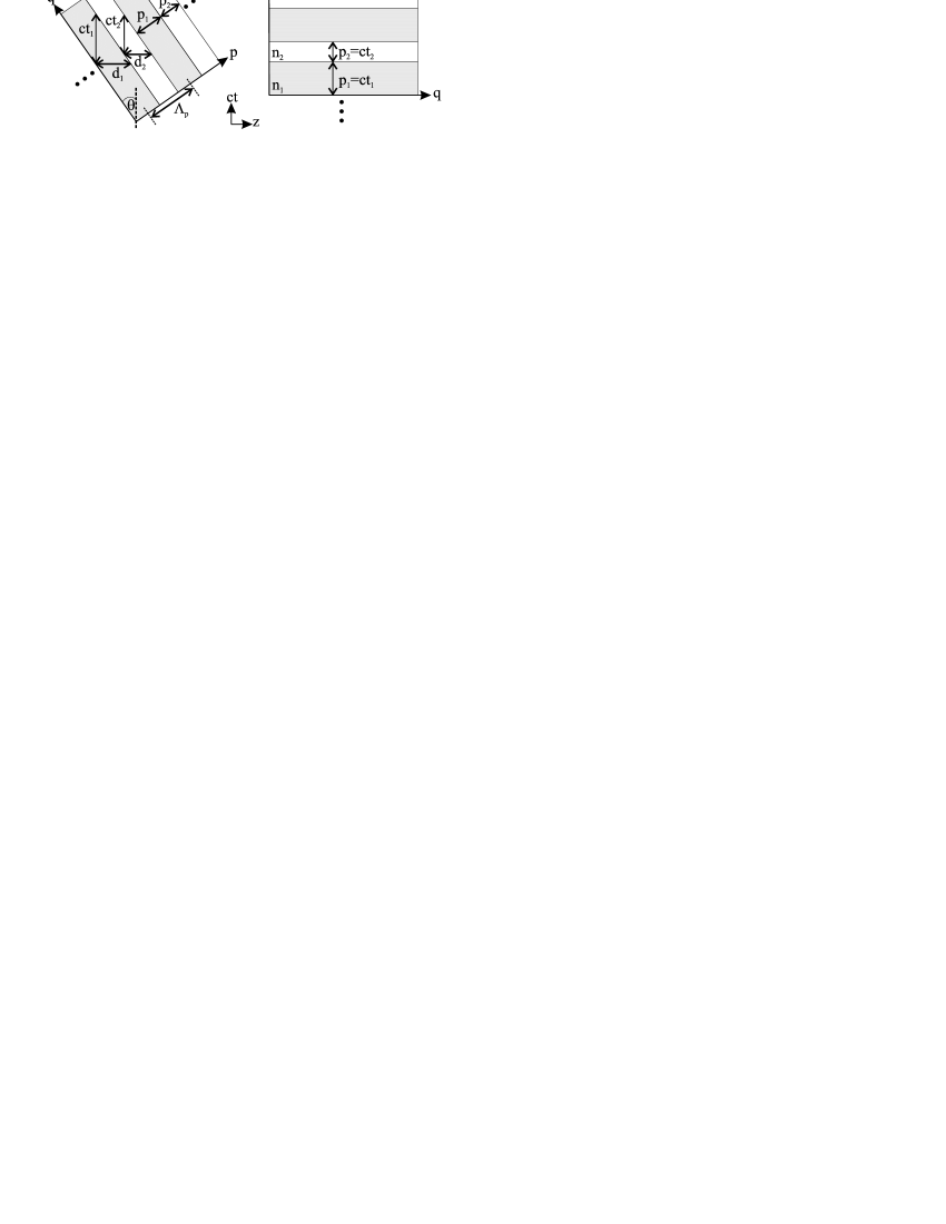
Figure 5: (a) Schematic figure showing the quantities of interest used in the text to define a general multilayer structure (with indices $n_{j}$, $j=\{1,2\}$) for an arbitrary angle $\theta$ (i.e. arbitrary parameter $\beta$). $p$ indicates the propagation direction for the Bloch waves, while $q$ is the delocalization direction for plane waves. $d_{j}$ are the widths of the layers along the $z$-direction, while $ct_{j}$ are the widths along the $ct$-direction. $p_{j}$ indicate the same quantities but along the $p$-direction. $\Lambda_{p}=p_{1}+p_{2}$ is the total length of the unit cell, also indicated in the figure. (b) Time-like photonic crystal. The refractive index varies only along the time axis, which therefore coincides with $p$. The coordinate $z$ coincides with $q$, therefore plane waves are spatially delocalized. For the structure to be a time-like Bragg reflector, which is totally reflective for a certain wavenumber bandgap, the condition $ct_{j}=n_{j}\lambda/4$ must hold, where $\lambda$ is the wavelength of the incident plane wave.

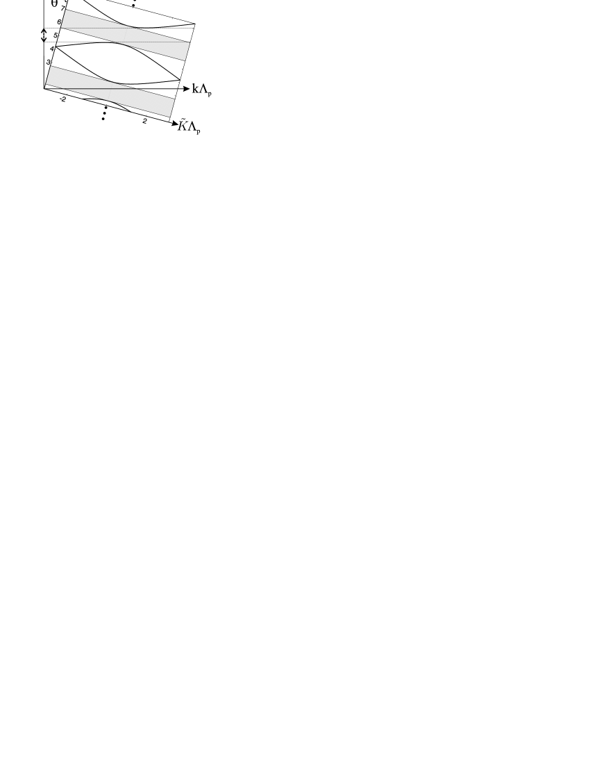
Figure 6: Bandstructure (solid lines) and bandgaps (grey areas) of a spatiotemporal Bragg reflector that satisfies the generalized quarter wavelength condition of Eq.(41), as calculated by using the transcendental photonic band equation Eq.(3.2). According to Eq.(24), the orthogonal axes $\tilde{\omega}$ and $\tilde{k}$ are rotated with respect to the orthogonal axes $\omega$ and $k$ by an angle $\theta$, as indicated in the figure. All quantities shown are dimensionless, and normalized in units of $\Lambda_{p}$. For $\theta=0$ (space-like photonic crystal), the two orthogonal bases would coincide, i.e. $\tilde{\omega}=\omega/c$ and $\tilde{k}=k$, and this corresponds to the case of a conventional, static photonic crystal. For a general $\theta$, the forbidden bandgaps in $\tilde{\omega}$ as calculated by Eq.(3.2) are shown by the grey areas. The projection of one of the bandgaps onto the axis $\omega$ is also shown, with its new smaller extension indicated by a dashed double-arrow. In the limit $\theta\rightarrow\pi/2$ (time-like photonic crystal), $\tilde{\omega}$ tends to $-k$, while $\tilde{k}$ tends to $\omega/c$, so that the forbidden gaps in $\tilde{\omega}$ will correspond to bandgaps in $k$. Note that there is a critical angle $\theta=\theta_{cr1}$ at which the projected $\omega$-gap will close, and a second critical angle $\theta_{cr2}>\theta_{cr1}$ at which the $k$-bandgaps start to open, until they reach their full extension at $\theta=\pi/2$.

3.3 Spatiotemporal Lenses, Pulse Compression and Broadening

Another interesting and potentially useful effect exhibited by a simple class of spatiotemporal dielectric structures is what we have called spatiotemporal lensing. Let us suppose that we have a refractive index distribution in the $(z,ct)$-plane of the form:

$$n(z,t)=n_{1}+(n_{2}-n_{1})\exp\left[-\left(\frac{t-t_{0}}{w_{t}/2}\right)^{2m_{t}}-\left(\frac{z-z_{0}}{w_{z}/2}\right)^{2m_{z}}\right].$$ (42)

In Eq.(42), $z_{0}$ and $t_{0}$ represent the coordinates of the center of the rectangular region, and $w_{z,t}$ are respectively its spatial and temporal extension, see Fig. 7. The two integer numbers $m_{z,t}$ model the sharpness of the supergaussian transitions between $n_{1}$ and $n_{2}$ along the spatial and temporal directions respectively. Eq.(42) models a rectangular region in the $(z,ct)$-space where the transition between an ’external’ refractive index $n_{1}$ and an ’internal’ index $n_{2}$ occurs, see Fig. 7. Here and in the following we shall refer to this region as a spatiotemporal lens, for reasons that will be clear shortly.

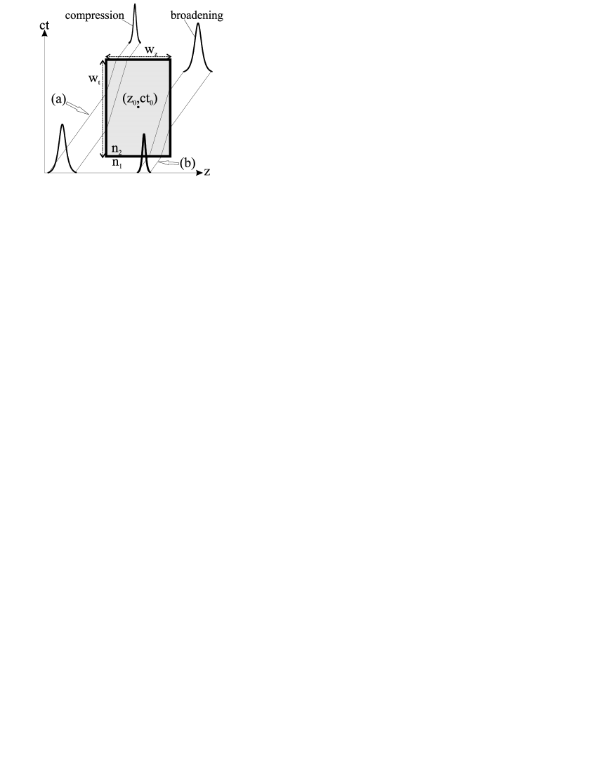
Figure 7: Schematic figure showing the mechanism of pulse compression [(a)] and pulse broadening [(b)] due to spatiotemporal lensing. The refractive index of the rectangular region shown is given by Eq. (42). The refractive indices outside the rectangle and inside it are uniform, in the $(z,ct)$-plane, and equal to $n_{1}$ and $n_{2}$ respectively. In this example we assume that $n_{2}>n_{1}$. During the scattering process every portion of the pulse will travel according to its local light cone, which is narrower in the grey region (light travels at speed $c/n_{2}<c/n_{1}$), and wider outside it. Backward waves produced in the scattering are not indicated in the figure for sake of clarity, but they are always present for sharp interfaces.

Fig. 7 illustrates the essential features of the scattering of a generic pulse by the rectangular spatiotemporal lens in the $(z,ct)$-plane. Essentially two configuration are of interest. In the first configuration [Fig. 7(a)], after some free propagation in the medium with index $n_{1}$, the pulse enters the grey region with index $n_{2}$ on the left side of the rectangular region, with the entire body of the pulse well inside the lateral extension of the rectangle ($w_{t}$). The pulse then propagates inside the structure, at a greater angle in the $(z,ct)$-plane, each portion of the pulse following the local light cone (defined in Fig. 1) at any instant of propagation. When the pulse exits the grey region, however, it is clear from Fig. 7(a) that its pulse duration has been reduced, and pulse compression has been achieved. It can be shown by elementary geometrical considerations that the compression ratio between the output and the input pulses in this simple case is just $\rho=n_{1}/n_{2}$. The scaling in the $(z,ct)$-plane is accompanied by an increase of the central frequency of the pulse by $1/\rho$, with a consequent increase of the spectral bandwidth. Thus we obtain an effective method for manipulating the frequency and wavenumber of a pulse.

The second scenario is when the pulse is delayed in such a way that it enters the spatiotemporal structure on the bottom side of the rectangle, the extension of which is $w_{z}$, and well inside it, see Fig. 7(b). This case shows exactly the opposite dynamics of the previous case, and pulse broadening in the $(z,ct)$-plane occurs by a factor of $\rho=n_{2}/n_{1}$. As a consequence the central frequency is reduced. This is of course not surprising due to the symmetry of Maxwell’s equations under the time reversal operation.

In Fig. 7 the backreflections at the interfaces, when the pulse enters the structure and when it leaves it, are not shown for simplicity, but it is clear from the discussions of the previous sections that for sharp interfaces of the structure they are always present.

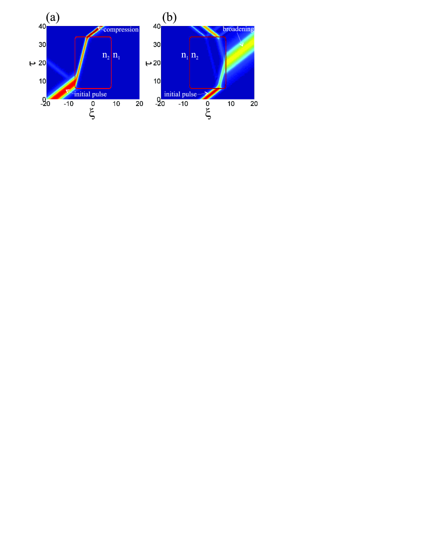
Figure 8: (Color online) Simulation showing pulse propagation and scattering by a spatiotemporal lens in the $(z,ct)$-plane which separates two regions with uniform refractive indices $n_{1}$ and $n_{2}$, as schematically described by Fig. 7. (a) A broad pulse [$w=3$ in Eq.(33)] hits the rectangle on the leftmost side, and pulse compression is achieved. (b) A short pulse [$w=1$ in Eq.(33)] hits the structure on the bottom side, and pulse broadening is achieved. For sake of clarity, only the interface of the rectangle is shown. Parameters of the simulations are: $n_{1}=1$, $n_{2}=3$, $z_{0}=0$, $ct_{0}=20\lambda$, $w_{t}=27\lambda$, $w_{z}=15\lambda$, $m_{t}=m_{z}=20$, and $\lambda$ is an arbitrary scale which we take equal to the central pulse wavelength. Horizontal axis is dimensionless space coordinate $\xi=z/\lambda$, while the vertical axis is dimensionless time coordinate $\tau=ct/\lambda$, and $\lambda$ is the central pulse wavelength.

The scenarios described above are confirmed by direct numerical simulations, see the panel of Fig. 8. Fig. 8(a) shows the evolution of a spatially and temporally broad input pulse [$w=3$ in Eq.(33)]. After hitting the leftmost side of the rectangular spatiotemporal region, the pulse emerges from the upper side considerably compressed, both in spatial and temporal domain. Only the interface of the $n_{2}$ region is indicated for sake of clarity, in order to clearly distinguish the internal wave propagation. Fig. 8(b) shows the compression dynamics, in which an input pulse with $w=1$ hits the structure on the bottom side. The pulse emerging from the right-hand side acquires a significant broadening. Several waves propagating backwards are noticeable in Fig. 8(a,b), and these are due to the sharpness of the interface region, which is modeled by Eq.(42) with the specific parameters given in the caption.

So far we have considered the extreme cases where both interfaces are space- or time-like. With the formalism developed in the previous section we can also consider the general case where a pulse enters a medium with refractive index $n_{2}$ via an interface characterized by an angle $\theta_{1}$ and leaves that medium via another interface characterized by an angle $\theta_{2}$. A straightforward geometrical analysis gives the rescaling factor in the $(z,ct)$-plane as

$$\rho=\left(\frac{\cos\theta_{2}-n_{1}\cos\theta_{1}}{\cos\theta_{2}-n_{2}\cos\theta_{1}}\right)\left(\frac{\sin\theta_{2}-n_{2}\sin\theta_{1}}{\sin\theta_{2}-n_{1}\sin\theta_{1}}\right)$$ (43)

which as expected reduces to $\rho=n_{1}/n_{2}$ ( $\rho=n_{2}/n_{1}$ ) for the previously considered cases $\theta_{1}=0$ and $\theta_{2}=\pi/2$ ($\theta_{2}=0$ and $\theta_{1}=\pi/2$).

4 Derivation of a Slow-Variable equation. Comparison with Eq.(2)

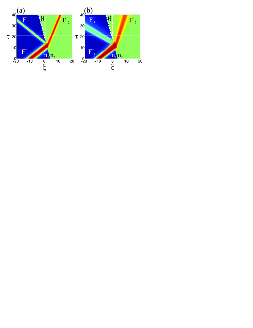
Figure 9: (Color online) Comparison between pulse evolution described by (a) the full Eq.(2) and (b) the approximate Eq.(45), which was derived under assumption of SVEA in time. The two simulations are carried out under absolutely identical conditions. Parameters are: $\beta=-0.2$, $\theta=-0.2027$, $w=1$, $n_{1}=1$ and $n_{2}=3$. In (b) one can notice an unphysical artificial broadening along the $z$-direction due to the uncompensated term proportional to the second derivative in space $\partial_{\xi}^{2}$ in Eq.(45). Horizontal axis is dimensionless space coordinate $\xi=z/\lambda$, while the vertical axis is dimensionless time coordinate $\tau=ct/\lambda$, and $\lambda$ is the central pulse wavelength.

From Eq.(1) it is possible to derive an equation for the electric field envelope function $A(z,t)$ only, which is of second order in the variables $z$ and $t$, by posing $E(z,t)=[A\exp(ik_{0}z-i\omega_{0}t)+\textrm{c.c.}]/2$, where $k_{0}=\omega_{0}/c$ and $\omega_{0}$ is an arbitrary frequency, usually and most conveniently chosen to be close to the central frequency of the input pulse. Using the dimensionless variables $\tau=ct/\lambda$, $\xi=z/\lambda$, where $\lambda=2\pi c/\omega_{0}$, and substituting the expression of the electric field $E$ into Eq.(1), we obtain:

$$\left(in^{2}-\frac{n\partial_{\tau}n}{\pi}\right)\partial_{\tau}A-\frac{n^{2}}{4\pi}(\partial^{2}_{\tau}A)+i\partial_{\xi}A+\frac{1}{4\pi}\partial_{\xi}^{2}A+$$

$$\pi\left[n^{2}-1+\frac{2in\partial_{\tau}n}{\pi}-\frac{(\partial_{\tau}n)^{2}}{2\pi^{2}}-\frac{n\partial_{\tau}^{2}n}{2\pi^{2}}\right]A=0.$$ (44)

Although Eq.(44) is written for the slow variable $A$, it is exact, and it is able to handle arbitrary pulses, and forward and backward propagation at the same time, due to the fact that it is completely equivalent to the full wave equation which can be derived from combining the two Maxwell equations of Eq.(1).

It is reasonable to conjecture that the use of the slowly varying envelope approximation (SVEA) in time in Eq.(44) is valuable in order to reduce the computational complexity of the problem. However, as we will show shortly, the use of SVEA in time but not in space is dangerous in that it leads to wrong results for pulse propagation, and this is especially important for the dielectric systems we are investigating in this paper, which show strong variations in the refractive index both in space and time. The use of SVEA in space in Eq.(44) is not permitted in particular when simulating sharp interfaces and photonic crystals, and in general in those systems in which the backward propagating waves are of the same order of magnitude of the forward propagating ones. Therefore all second derivatives $\partial_{\xi}^{2}$ must be maintained in Eq.(44).

Assuming that the central frequency of the pulse $\omega_{0}$ is much greater than the variation of the envelope function $A$ in time, we can perform a multiple scale reduction of Eq.(44), obtaining the following first order equation in time:

$$in^{2}\partial_{\tau}A+i\partial_{\xi}A+\frac{1}{4\pi}\partial_{\xi}^{2}A+\pi\left[n^{2}-1+\frac{2in\partial_{\tau}n}{\pi}\right]A=0.$$ (45)

Eq.(45) is a generalization to time-dependent refractive index of the propagation equation used in a series of works [17], where temporal variations of $n$ were not taken into account. Eq.(45) shows that the purely real ’Schroedinger potential’ $n^{2}-1$ used in [17] is modified by a purely imaginary term proportional to the time derivative of the refractive index, namely $i\partial_{\tau}n^{2}/\pi$.

Fig. 9 shows the comparison between the scattering of a pulse by a sharp interface, when calculated by means of the full Eqs.(2) [Fig. 9(a)] and by means of the approximate equation Eq.(45) [see Fig. 9(b)], under absolutely identical conditions. Although the two equations give very similar results for what concerns the transmission and reflection coefficients, the most striking difference between the pulse evolution in the two cases is the presence of a fictitious and unphysical broadening along the $z$-direction in Fig. 9(b). This is due to the fact that the use of SVEA in time but not SVEA in space in Eq.(45) leads to an uncompensated ’diffractive’ term proportional to $\partial_{\xi}^{2}A$, which is responsible for the broadening observed in Fig. 9(b) for all waves participating in the scattering.

The above considerations provide a justification of the use of the full Maxwell equations throughout the present paper, instead of equations using slow variables.

5 Discussion and Conclusions

Before concluding, we would like to spend a few words on the experimental relevance of the topics discussed in the present paper.

Many theoretical and experimental results exist in the literature, that discuss the interaction of electromagnetic pulses with a plasma front [19, 20, 21, 22, 23, 24]. This interaction has been typically used in practice to shift the central frequency of an incident pulse by means of the effect discussed in Section 3.3, see Refs. [21], or to convert static electric fields into electromagnetic pulses by means of a capacitor array [23]. These effects may turn out to be extremely useful in the creation of efficient tunable laser sources [19]. For instance, in typical experiments [20], when a ’probe’ pulse is propagating along the longitudinal coordinate of a semiconductor waveguide, one can change the refractive index of the material along all its spatial extension by means of irradiating the plane of the crystal with another ’source’ pulse that creates a electron-hole plasma throughout the crystal. If the source pulse has a certain angle of incidence $\alpha$ with respect to the normal to the plane of the waveguide, then the ionization front of the plasma will move with velocity $v=c/\sin(\alpha)$ [19, 24]. Note that for normal incidence ($\alpha=0$), this front moves instantaneously, and it corresponds to the time-like interface ($\theta\rightarrow\pi/2$, where the general relation between $\theta$ and $\alpha$ is $\theta+\alpha=\pi/2$) discussed in Section 3.1, which follows from a simultaneous change of refractive index throughout all the spatial extension of the crystal. This front does not carry any information, and it is not associated to any moving object, therefore its propagation is not limited by the speed of light in vacuum. In all these cases, none of the actual particles in the excited medium is moving faster than $c$; instead, the front profile only has an apparent motion, which can be characterized by an effective velocity given by the above formula, but does not correspond by any means to any real superluminal motion of particles or information, which is of course forbidden by special relativity. In this sense, $n(z,t)$ can be a totally arbitrary function with no relation whatsoever to moving bodies. In another kind of experiments [24], short pulses of the order of nanoseconds are created by irradiating a metal surface by X-rays at a certain angle of incidence $\alpha$, which creates a photoelectric current. Again, this current undergoes an apparent motion at a velocity $v=c/\sin(\alpha)$ and, by means of superluminal self-phasing of the excited elementary dipoles (predicted by Carron and Longmire in 1976 [24]), emits a short electromagnetic pulse at the same angle $\alpha$. It is also interesting to point out that the processes described briefly above can also have considerable implications for the physics of astrophysical plasmas [23].

A remark which is important for the present work is that it is assumed that the physical experiments well approximate a condition of quasi-one-dimensional propagation of the incident probe pulse, therefore implying a well-localized confinement of the transverse profile by means of a strong waveguiding process which does not allow diffraction, so that the equations we have derived in this paper, having the transverse ($x$, $y$) and the longitudinal ($z$) degrees of freedom decoupled, can be safely utilized.

In conclusion, in this paper the physics of light propagation scattered by nonstationary interfaces has been investigated analytically and numerically in a unified approach. Interface transfer matrix and propagation matrix have been found for the general case of arbitrary velocities of the interface. These ingredients have been used to construct more complicated spatiotemporal dielectric structures. In particular, we have first investigated a spatiotemporal Bragg reflector, where we have given the generalized condition for the existence of forbidden bandgaps, and found that the frequency bandgaps close for a critical value of $\theta=\theta_{cr1}$, with the successive opening of the wavenumber bandgap at a second critical angle $\theta=\theta_{cr2}$. Secondly we have explored light scattering by a spatiotemporal lens device, and the spectral manipulation of pulses has been demonstrated both analytically and numerically, the most important aspect of which is a potentially strong pulse compression/broadening.

Future works include the natural extension of the theory given here to a dispersive susceptibility.

This research has been supported by Science Foundation Ireland (SFI) and the Irish Research Council for Science, Engineering and Technology (IRCSET).

References

- [1] W. C. Chew, Waves and Fields in Inhomogeneous Media (Wiley-IEEE Press, 1999).
- [2] P. Yeh, Optical Waves in Layered Media (Wiley and Sons, N.Y., 2005).
- [3] J. D. Jackson, Classical Electrodynamics (Wiley and Sons, New York, 1975).
- [4] L. D. Landau and E. M. Lifshits, Electrodynamics of Continuous Media (Pergamon Press, Oxford, 1960).
- [5] C. Yeh and K. F. Casey, Phys. Rev. 144, 665 (1966); C. Yeh, Phys. Rev. 167, 875 (1968); Phys. Rev. E 48, 1426 (1993).
- [6] J. M. Saca, J. Mod. Opt. 36, 1367 (1989).
- [7] Y. X. Huang, J. Mod. Opt. 44, 623 (1997).
- [8] M. Visser, Class. Quant. Grav. 15, 1767 (1998); Phys. Rev. Lett. 85, 5252 (2000).
- [9] U. Leonhardt and P. Piwnicki, Phys. Rev. Lett. 82, 2426 (1999); Phys. Rev. A 60, 4301 (1999); Phys. Rev. Lett. 84, 822 (2000); Phys. Rev. A 62, 055801 (2000); J. Mod. Opt. 48, 977 (2001); Appl. Phys. B 72, 51 (2001).
- [10] F. De Felice, Gen. Rel. and Grav. 2, 347 (1971).
- [11] L. A. Ostrovsky, Sov. Phys. Uspekhi 18, 452 (1975).
- [12] F. R. Morgenthaler, IRE Trans. Microwave Theory Tech. MTT-6, 167 (1958).
- [13] L. B. Felsen and G. M. Whitman, IEEE Trans. Antennas Propagat. AP-18, 242 (1970).
- [14] R. L. Fante, IEEE Trans. Antennas Propagat. AP-19, 417 (1971).
- [15] A. B. Shvartsburg, Physics Uspekhi 48, 797 (2005).
- [16] M. Nakahara, Geometry, Topology, and Physics (2nd ed., Taylor and Francis, London, 2003).
- [17] J. P. Dowling, M. Scalora, M. J. Bloemer and C. M. Bowden, J. Appl. Phys 75, 1896 (1994); M. Scalora, J. P. Dowling, C. M. Bowden and M. J. Bloemer, Phys. Rev. Lett. 73, 1368 (1994); M. Scalora and M. E. Crenshaw, Opt. Commun. 108, 191 (1994); M. Scalora, J. P. Dowling, C. M. Bowden and M. J. Bloemer, J. Appl. Phys. 76, 2023 (1994); M. Scalora, M. J. Bloemer, A. S. Manka, J. P. Dowling, C. M. Bowden, R. Viswanathan and J. W. Haus, Phys. Rev. A 56, 3166 (1997).
- [18] S. Mishra and S. Satpathy, Phys. Rev. B 68, 045121 (2003).
- [19] V. I. Berezhiani, S. M. Mahajan, and R. Miklaszewski, Phys. Rev. A 59, 859 (1999).
- [20] Y. Avitzour, I. Geltner and S. Suckewer, J. Phys. B: At. Mol. Opt. Phys. 38, 779 (2005).
- [21] S. C. Wilks, J. M. Dawson and W. B. Mori, Phys. Rev. Lett. 61, 337 (1988); R. L. Savage, C. Joshi and W. B. Mori, Phys. Rev. Lett. 68, 946 (1992); I. Geltner, Y. Avitzour and S. Suckewer, Appl. Phys. Lett. 81, 226 (2002).
- [22] M. Lampe, E. Ott and J. H. Walker, Phys. Fluids 21, 42 (1978).
- [23] D. Hashimshony, A. Zigler and K. Papadopoulos, Phys. Rev. Lett. 86, 2806 (2001); C. H. Lai, R. Liou, T. C. Katsouleas, P. Muggli, R. Brogle, C. Joshi and W. B. Mori, Phys. Rev. Lett. 77, 4764 (1996).
- [24] N. J. Carron and C. L. Longmire, IEEE Trans. Nucl. Sci. NS-23, 1897 (1976); A. V. Bessarab, A. A. Gorbunov, S. P. Martynenko and N. A. Prudkoy, IEEE Trans. Plasma Sci. 32, 1400 (2004).